Sampling theorem and efficiency comparison of three local minimum variance unbiased estimators of the mean and variance of the exponential distribution

Abstract

This article continues the works of references to improve and perfect the sampling theorem of exponential distribution. First, the distribution of the sample range of exponential distribution is derived, and that the sample range is mutually independent of the sample minimum is proven. Then, this article derives the distribution of the difference between sample maximum and mean and demonstrates that the difference of these two statistics is mutually independent of the sample minimum. Thus, three local minimum variance unbiased estimators of the mean could be constructed. The estimator built by sample minimum and the difference between sample mean and minimum is precisely the uniformly minimum-variance unbiased estimator (UMVUE) of the mean. Similarly, three local minimum variance unbiased estimators of the variance are derived. At last, the efficiency comparison is made among the above three local minimum variance unbiased estimators of mean and variance of the exponential distribution.

Keywords:

• sampling theorem of exponential distribution
• local minimum variance unbiased estimators
• mean
• variance
• UMVUE
• efficiency
• sample mean
• sample minimum
• sample maximum
• difference

MR Subject classifications:

• 62D05
• 62E15
• 62F10

PUBLIC INTEREST STATEMENT

What is the sampling theorem of the exponential distribution? It includes the content about the distributions of the sample mean, sample maximum, sample minimum and their differences. It also includes the content of whether their differences are mutually independent of sample minimum. What is the local minimum variance unbiased estimation? Based on two mutually independent unbiased estimators, a kind of weighted linear unbiased estimators could be constructed, among which the one with the minimum variance is the local minimum variance unbiased estimation. One should remember that three local minimum variance unbiased estimators of mean and variance are not substituted for uniformly minimum variance unbiased estimators of mean and variance, respectively, but only rich in natural estimators.

1. Introduction

Sample minimum, sample maximum and sample mean are important statistics in exponential distribution. Sample minimum has an exponential distribution, and sample mean has a gamma distribution or Chi-square distribution with degree freedom of n. The difference of sample mean and minimum has a gamma distribution or Chi-square distribution with degree freedom of n–1. The difference between sample mean and minimum is mutually independent of the sample minimum (Arnold, 1968; Gupta & Kundu, 0000; Marshall & Olkin, 1967).

This article derives the distribution of the sample range and demonstrates that the sample range is mutually independent of sample minimum. Then, the distribution of the difference between sample maximum and mean is derived, and that the difference of these two statistics is mutually independent of the sample minimum is demonstrated (Cohen and Helm, 1973; Kundu & Gupta, 2009; Lawrance & Lewis, 1983; Nie, Sinha, & Hedayat, 2017).

Thus, the sampling theorem is improved. As natural corollary of the sampling theorem of the exponential distribution, a first local minimum variance unbiased estimators of expectation could be constructed by sample minimum and the difference between sample mean and minimum, which is precisely the UMVUE of the expectation. A second local minimum variance unbiased estimators of expectation could be constructed by sample minimum and sample range. A third local minimum variance unbiased estimators of expectation could be constructed by sample minimum and the difference between sample maximum and mean; similarly, three local minimum variance unbiased estimators of the variance are derived. At last, the efficiency comparison is made among the above three local minimum variance unbiased estimators of mean and variance of the exponential distribution (Al-Saleh & Al-Hadhrami, 2003; Baklizi & Dayyeh, 2003; Dixit & Nasiri, 2008; Guoan, Jianfeng, & Lihong, 2017; Li, 2016).

2. Sampling theorem of exponential distribution

The joint distribution of order statistics $(X_{(1)},...,X_{(n)})$ of exponential distribution is shown as follows:

Definition 2.1. If $X\sim E(\alpha )$, $X_1,...,X_n$ is a sample with sample size $n$ from $X\sim E(\alpha )$, $(X_{(1)},...,X_{(n)})$has a joint density function:

(1) $f(x_{(1)},x_{(2)},...,x_{(n)})=\frac{n!}{{\alpha }^n}exp[-\frac{{\sum }_1^n{x}_{(i)}}{\alpha }],x_{(1)}<x_{(2)}...<x_{(n)},\alpha >0$(1)

Then, we could say $(X_{(1)},...,X_{(n)})$ is from a multivariate order statistics exponential distribution.

Notate $n\bar{X}={\sum }_1^n{X}_i={\sum }_1^n{X}_{(i)}$, the sampling theorem is:

Theorem 2.1. If $X\sim E(\alpha )$, $X_1,...,X_n$ is a sample from $X\sim E(\alpha )$ with sample size $n$, $(X_{(1)},...,X_{(n)})$ are the order statistics, then

(1) $\frac{2n{X}_{(1)}}{\alpha }\sim {\chi }^2(2)$,$\frac{2n(\bar{X}-X_{(1)})}{\alpha }\sim {\chi }^2(2(n-1))$, $\bar{X}-X_{(1)}$ is mutually independent of $X_{(1)}$.

(2) $-2(n-1)ln\left(1-exp\left[-\frac{(X_{(n)}-X_{(1)})}{\alpha }\right]\right)\sim {\chi }^2(2)$, $X_{(1)}$ is mutually independent of $(X_{(n)}-X_{(1)})$.

(3) $X_{(1)}$ is mutually independent of $(X_{(n)}-\bar{X})$. The density function of $(X_{(n)}-\bar{X})$:

(2) $f_{(X_{(n)}-\overline{X})}(x)={\displaystyle {\sum }_0^{n-2}{(-1)}^k}{\text{C}}_{\text{n-1}}^{\text{k}}\frac{{(\text{n-1-k})}^{\text{n-2}}(\text{n-1})}{{\text{n}}^{\text{n-2}}\alpha }\exp \left(\text{-}\frac{(\text{n-1})(\text{k+1})\text{x}}{(\text{n-1-k})\alpha }\right),\text{x>0}$(2)

Proof. $P(X_{(1)}>x_{(1)})=P(X_1>x_{(1)},...,X_n>x_{(1)})=exp[-\frac{n{x}_{(1)}}{\alpha }]$,

$g(x_{(1)})=\frac{n}{\alpha }{e}^{-\frac{n{x}_{(1)}}{\alpha }},x_{(1)}>0,\frac{2n{X}_{(1)}}{\alpha }\sim {\chi }^2(2).$

Notate $U_{(i-1)}=X_{(i)}-X_{(1)},i=2,...,n$, $V=X_{(1)}$,

$u_{(i-1)}=x_{(i)}-x_{(1)},v=x_{(1)}\Rightarrow x_{(i)}=u_{(i-1)}+v,i=2,\dots ,n.x_{(1)}=v,$

the joint distribution density of $(U_{(1)},...,U_{(n-1)},V)$ is:

(2.3) $f(u_{(1)},u_{(2)},...,u_{(n-1)},v)=\frac{(n)!}{{\alpha }^n}exp\left[-\frac{({\sum }_1^{n-1}{u}_{(i)}+nv)}{\alpha }\right],u_{(1)}<u_{(2)}...<u_{(n-1)},v>0$(2.3)

Therefore, $(U_{(1)},U_{(2)}...,U_{(n-1)})$ is the order statistics of sample $(U_1,U_2...,U_{n-1})$, which is the sample from $U\sim E(\alpha )$ with sample size$n-1$,$(U_1,U_2,...,U_{n-1})$ is mutually independent of $X_{(1)}$.

$\frac{2(n\bar{X}-n{X}_{(1)})}{\alpha }=\frac{2(\sum _1^n{X}_{(i)}-n{X}_{(1)})}{\alpha }=\frac{2(\sum _1^{n-1}{U}_i)}{\alpha }\sim {\chi }^2(2(n-1))$, $\bar{X}-X_{(1)}$ is mutually independent of $X_{(1)}$.

Then, prove part (2).

$F_{(X_{(1)},X_{(n)})}(x,y)=P(X_{(1)}>x,X_{(n)}\le y)=P(x<X_1\le y,\dots ,x<X_n\le y)={\left[exp\left(-\frac{x}{\alpha }\right)-exp\left(-\frac{y}{\alpha }\right)\right]}^n$

(2.4) $f_{(X_{(1)},X_{(n)})}(x,y)=\frac{n(n-1)}{{\alpha }^2}{\left[exp\left(-\frac{x}{\alpha }\right)-exp\left(-\frac{y}{\alpha }\right)\right]}^{n-2}exp\left[-\frac{(x+y)}{\alpha }\right]$(2.4)

Transform as $U_1=X_{(1)},U_2=X_{(n)}-X_{(1)}$,

(2.5) $f_{(U_1,U_2)}(u_1,u_2)=\frac{n(n-1)}{{\alpha }^2}{\left[exp\left(-\frac{u_1}{\alpha }\right)-exp\left(-\frac{(u_1+u_2)}{\alpha }\right)\right]}^{n-2}exp\left[-\frac{(2u_1+u_2)}{\alpha }\right]$(2.5)

$f_{U_1}(u_1)=\frac{n}{\alpha }exp[-\frac{n{u}_1}{\alpha }]$, $f_{U_2}(u_2)=\frac{(n-1)}{\alpha }[1-exp(-\frac{u_2}{\alpha }){]}^{n-2}exp[-\frac{u_2}{\alpha }]$.

Therefore, $U_1$ is mutually independent of $U_2$.

$\frac{2n{X}_{(1)}}{\alpha }\sim {\chi }^2(2)$, $-2(n-1)ln\left(1-exp\left[-\frac{(X_{(n)}-X_{(1)})}{\alpha }\right]\right)\sim {\chi }^2(2)$.

Notate $U_{(i-1)}=X_{(i)}-X_{(1)},i=2,...,n$, $W_{(1)}=U_{(1)}$,

$W_{(k)}=k{U}_{(k)}-{\sum }_1^{k-1}{U}_{(i)},k=2,...,n-1$, then $W_{(2)}-W_{(1)}=2U_{(2)}-2U_{(1)}>0$,

$W_{(k)}-W_{(k-1)}=k{U}_{(k)}-(k-1)U_{(k-1)}-U_{(k-1)}=k(U_{(k)}-U_{(k-1)})>0,k=2,...,n-1$, the determinant is:

(2.6) $\left|J\right|=\left|\begin{array}{ccccc}1& 0& 0& ...& 0\\ -1& 2& 0& ...& 0\\ -1& -1& 3& ...& 0\\ ...& ...& ...& ...& ...\\ -1& -1& -1& ...& n-1\end{array}\right|=(n-1)!$(2.6)

In ${\sum }_1^{n-1}{U}_{(i)}$, the coefficient of $W_{(k)}$ is $\frac{n}{k(k+1)}$, $k=1,...,n-2$, the coefficient of $W_{(n-1)}$ is $\frac{1}{(n-1)}$. Derive the density function $f_{W_{(n-1)}}(w_{(n-1)})$ of $W_{(n-1)}$:

(2.7) $\begin{array}{rl}& f_{W_{(n-1)}}(w_{(n-1)})={\int }_0^{w_{(n-1)}}d{w}_1{\int }_{w_{(1)}}^{w_{(n-1)}}d{w}_2...{\int }_{w_{(n-4)}}^{w_{(n-1)}}d{w}_{n-3}{\int }_{w_{(n-3)}}^{w_{(n-1)}}\frac{exp[-\frac{w_{(n-1)}}{(n-1)\alpha }]}{{\alpha }^{n-1}}exp\left[-\frac{{\sum }_1^{n-2}\frac{n{w}_{(k)}}{k(k+1)}}{\alpha }\right]d{w}_{n-2}\\ & =\left\{\frac{{(n-1)}^{n-2}}{n^{n-2}}-\frac{{(n-2)}^{n-2}(n-1)}{n^{n-2}}exp\left[-\frac{nw}{(n-1)(n-2)\alpha }\right]+\frac{(n-1)(n-2)}{2}\frac{{(n-3)}^{n-2}}{{(n)}^{n-2}}\right.\\ & exp\left[-\frac{2nw}{(n-1)(n-3)\alpha }\right]-\frac{(n-1)(n-2)(n-3)}{3\times 2\times 1}\frac{{(n-4)}^{n-2}}{{(n)}^{n-2}}exp\left[-\frac{3nw}{(n-1)(n-4)\alpha }\right]+...\\ & \left.+(-1{)}^{n-2}\frac{(n-1)}{n^{n-2}}exp\left[-\frac{n(n-2)w}{(n-1)\alpha }\right]\right\}\frac{1}{\alpha }exp\left[-\frac{w}{(n-1)\alpha }\right],w>0\end{array}$(2.7)

From $W_{(n-1)}=(n-1)(X_{(n)}-\bar{X})$, we could obtain $f_{(X_{(n)}-\bar{X})}(x)=(n-1)f_{W_{(n-1)}}((n-1)x)$, then obtain:

$f_{(X_{(n)}-\overline{X})}(x)=\frac{{(n-1)}^{n-2}}{n^{n-2}}+\frac{{(-1)}^1{C}_{n-1}^1{(n-2)}^{n-2}}{n^{n-2}}\exp [-\frac{nx}{(n-2)\alpha }]+\frac{{(-1)}^2{C}_{n-1}^2{(n-3)}^{n-2}}{{(n)}^{n-2}}$

$\exp \left[-\frac{2nx}{(n-3)\alpha }\right]+\frac{{(-1)}^3{C}_{n-1}^3{(n-4)}^{n-2}}{{(n)}^{n-2}}\exp \left[-\frac{3nx}{(n-4)\alpha }\right]+\dots +\frac{{(-1)}^{n-2}{C}_{n-1}^{n-2}}{n^{n-2}}\exp \left[-\frac{n(n-2)x}{\alpha }\right]$

$\frac{(n-1)}{\alpha }\exp \left[-\frac{x}{\alpha }\right]\text{=}{\displaystyle {\sum }_0^{n-2}{(-1)}^k}{\text{C}}_{n\text{-1}}^{\text{k}}\frac{{(\text{n-1-k})}^{n\text{-2}}}{n^{\text{n-2}}}\exp \left[\text{-}\frac{\text{knx}}{(n\text{-1-k})\alpha }\right]\frac{(n\text{-1})}{\alpha }\exp \left[\text{-}\frac{\text{x}}{\alpha }\right]$

(2.8) $={\displaystyle {\sum }_0^{n-2}{(-1)}^k}{\text{C}}_{n\text{-1}}^{\text{k}}\frac{{(\text{n-1-k})}^{n\text{-2}}(\text{n-1})}{n^{\text{n-2}}\alpha }\exp (\text{-}\frac{(n\text{-1})(\text{k+1})\text{x}}{(n\text{-1-k})\alpha }),\text{x}\text{<0}.$(2.8)

List some specific situations:

When $n=3$:

$f_{(X_{(3)}-\bar{X})}(x)=\left[\frac{4}{3\alpha }exp(-\frac{x}{\alpha })-\frac{4}{3\alpha }exp(-\frac{4x}{\alpha })\right],x>0$, it is a mixed exponential distribution.

When $n=4$:

$f_{(X_{(4)}-\bar{X})}(x)=\left[\frac{27}{16\alpha }exp(-\frac{x}{\alpha })-\frac{9}{4\alpha }exp(-\frac{3x}{\alpha })+\frac{9}{16\alpha }exp(-\frac{9x}{\alpha })\right],x>0,$

When $n=5$:

$f_{(X_{(5)}-\overline{X})}(x)=\frac{256}{125\alpha }\exp \left(-\frac{x}{\alpha }\right)-\frac{432}{125\alpha }\exp \left(-\frac{8x}{3\alpha }\right)+\frac{192}{125\alpha }\exp \left(-\frac{6x}{\alpha }\right)-\frac{16}{125\alpha }\exp \left(-\frac{16x}{\alpha }\right)],x\text{<}0,$

When $n=6$:

$f_{(X_{(6)}-\bar{X})}(w)=\left[\frac{3125}{1296\alpha }exp(-\frac{x}{\alpha })-\frac{400}{81\alpha }exp(-\frac{5x}{2\alpha })+\frac{25}{8\alpha }exp(-\frac{5x}{\alpha })-\frac{50}{81\alpha }exp(-\frac{10x}{\alpha })+\frac{25}{1296\alpha }exp(-\frac{25x}{\alpha })\right],x>0$$X_{(1)}$ is mutually independent of$(X_{(n)}-\bar{X})$.

3. Three local minimum variance unbiased estimators of expectation

Theorem 3.1. If $X\sim E(\alpha )$, $X_1,...,X_n$ is the sample from $X\sim E(\alpha )$ with sample size${ }^n$, $X_{(1)},...,X_{(n)}$ are the order statistics, then the local minimum variance unbiased estimator, which is based on $X_{(1)}$and $\bar{X}-X_{(1)}$, is the UMVUE of expectation.

Proof. From Theorem 2.1: $\frac{2n{X}_{(1)}}{\alpha }\sim {\chi }^2(2)$, $\frac{2n(\bar{X}-X_{(1)})}{\alpha }\sim {\chi }^2(2(n-1))$, $\bar{X}-X_{(1)}$ is mutually independent of $X_{(1)}$, we obtain $n{X}_{(1)}$ and $\frac{n(\bar{X}-X_{(1)})}{n-1}$are both unbiased estimator of $\alpha$, and the effective unbiased estimator is ${\hat{\alpha }}_0=c(n{X}_{(1)})+(1-c)\frac{n(\bar{X}-X_{(1)})}{n-1}$,

(3.1) $\mathrm{h}\mathrm{e}\mathrm{r}\mathrm{e}c=\frac{D(\frac{n(\bar{X}-X_{(1)})}{n-1})}{D(n{X}_{(1)})+D(\frac{n(\bar{X}-X_{(1)})}{n-1})}=\frac{\frac{{\alpha }^2}{(n-1)}}{{\alpha }^2+\frac{{\alpha }^2}{(n-1)}}=\frac{1}{n},$(3.1)

Plug in and get ${\hat{\alpha }}_0=\bar{X}$, which is the UMVUE of the expectation.

Theorem 3.2. If $X\sim E(\alpha )$, $X_1,...,X_n$ is the sample from $X\sim E(\alpha )$ with sample size $n$, $X_{(1)},...,X_{(n)}$ are the order statistics, then the local minimum variance unbiased estimator, which is based on $X_{(1)}$ and $(X_{(n)}-X_{(1)})$, is ${\hat{\alpha }}_1=c_1{\hat{\alpha }}_{11}+(1-c_1){\hat{\alpha }}_{12}$, here

(3.2) $c_1=\frac{2\left[{\sum }_1^{n-1}\frac{{(-1)}^{k+1}{C}_{n-1}^k}{k^2}\right]-{\left[{\sum }_1^{n-1}\frac{{(-1)}^{k+1}{C}_{n-1}^k}{k}\right]}^2}{{\left[{\sum }_1^{n-1}\frac{{(-1)}^{k+1}{C}_{n-1}^k}{k}\right]}^2+2\left[{\sum }_1^{n-1}\frac{{(-1)}^{k+1}{C}_{n-1}^k}{k^2}\right]-{\left[{\sum }_1^{n-1}\frac{{(-1)}^{k+1}{C}_{n-1}^k}{k}\right]}^2}$(3.2)

${\hat{\alpha }}_{11}$ is the unbiased estimator based on $X_{(1)}$, ${\hat{\alpha }}_{11}=n{X}_{(1)}$, ${\hat{\alpha }}_{12}$ is the unbiased estimator based $(X_{(n)}-X_{(1)})$: ${\hat{\alpha }}_{12}=\frac{X_{(n)}-X_{(1)}}{{\sum }_1^{n-1}\frac{{(-1)}^{k+1}{C}_{n-1}^k}{k}}$.

Proof. $E(X_{(n)}-X_{(1)})={\int }_0^{\mathrm{\infty }}x\frac{n-1}{\alpha }[1-exp(-\frac{x}{\alpha }){]}^{n-2}exp(-\frac{x}{\alpha })dx=-x[1-(1-exp(-\frac{x}{\alpha }){)}^{n-1}]|\begin{array}{c}\mathrm{\infty }\\ 0\end{array}$

$+{\int }_0^{\mathrm{\infty }}[1-(1-exp(-\frac{x}{\alpha }){)}^{n-1}]dx={\int }_0^{\mathrm{\infty }}[{\sum }_1^{n-1}(-1{)}^{k+1}{C}_{n-1}^{k}exp(-\frac{kx}{\alpha })]dx={\sum }_1^{n-1}\frac{{(-1)}^{k+1}{C}_{n-1}^k\alpha }{k}$, $E{\hat{\alpha }}_{12}=E(\frac{X_{(n)}-X_{(1)}}{\sum _1^{n-1}\frac{{(-1)}^{k+1}{C}_{n-1}^k}{k}})=\alpha$, from Theorem 2.1: ${\hat{\alpha }}_{11}$ is independent of ${\hat{\alpha }}_{12}$, ${\hat{\alpha }}_{11}$ and ${\hat{\alpha }}_{12}$ are both unbiased estimator of $\alpha$, when $0\le c_1\le 1$, ${\hat{\alpha }}_1=c_1{\hat{\alpha }}_{11}+(1-c_1){\hat{\alpha }}_{12}$ is the unbiased estimator of $\alpha$, $D(c_1{\hat{\alpha }}_{11}+(1-c_1){\hat{\alpha }}_{12})=c_1^{2}D({\hat{\alpha }}_{11})+(1-c_1{)}^{2}D({\hat{\alpha }}_{12})$, take derivative of $c_1$, make it equal to 0 and get: $2c_{1}D({\hat{\alpha }}_{11})-2(1-c_1)D({\hat{\alpha }}_{12})=0\Rightarrow c_1=\frac{D({\hat{\alpha }}_{12})}{D({\hat{\alpha }}_{11})+D({\hat{\alpha }}_{12})}$,

here, $D{\hat{\alpha }}_{11}=Dn{X}_{(1)}=\frac{{\alpha }^2}{4}D\frac{2n{X}_{(1)}}{\alpha }=\frac{{\alpha }^2}{4}\times 2\times 2={\alpha }^2$,

$E(X_{(n)}-X_{(1)}{)}^2={\int }_0^{\mathrm{\infty }}{x}^2\frac{n-1}{\alpha }{\left[1-exp(-\frac{x}{\alpha })\right]}^{n-2}exp(-\frac{x}{\alpha })dx=-x^2\left[1-(1-exp(-\frac{x}{\alpha }){)}^{n-1}\right]|\begin{array}{c}\mathrm{\infty }\\ 0\end{array}+$

${\int }_0^{\mathrm{\infty }}2x[1-(1-exp(-\frac{x}{\alpha }){)}^{n-1}]dx=2{\int }_0^{\mathrm{\infty }}[{\sum }_1^{n-1}(-1{)}^{k+1}{C}_{n-1}^{k}xexp(-\frac{kx}{\alpha })]dx=2{\sum }_1^{n-1}\frac{{(-1)}^{k+1}{C}_{n-1}^k{\alpha }^2}{k^2},$

$D(X_{(n)}-X_{(1)})=2\left[{\sum }_1^{n-1}\frac{{(-1)}^{k+1}{C}_{n-1}^k{\alpha }^2}{k^2}\right]-{\left[{\sum }_1^{n-1}(C_{n-1}^k(-1{)}^{k+1}\frac{\alpha }{k})\right]}^2,$

$D{\hat{\alpha }}_{12}=D\frac{(X_{(n)}-X_{(1)})}{\left[{\sum }_1^{n-1}\frac{{(-1)}^{k+1}{C}_{n-1}^k}{k}\right]}=\frac{2\left[{\sum }_1^{n-1}\frac{{(-1)}^{k+1}{C}_{n-1}^k{\alpha }^2}{k^2}\right]-{\left[{\sum }_1^{n-1}(C_{n-1}^k{(-1)}^{k+1}\frac{\alpha }{k})\right]}^2}{{\left[{\sum }_1^{n-1}\frac{{(-1)}^{k+1}{C}_{n-1}^k}{k}\right]}^2},$

when $c_1=\frac{2\left[{\sum }_1^{n-1}\frac{{(-1)}^{k+1}{C}_{n-1}^k}{k^2}\right]-{\left[{\sum }_1^{n-1}\frac{{(-1)}^{k+1}{C}_{n-1}^k}{k}\right]}^2}{{\left[{\sum }_1^{n-1}\frac{{(-1)}^{k+1}{C}_{n-1}^k}{k}\right]}^2+2\left[{\sum }_1^{n-1}\frac{{(-1)}^{k+1}{C}_{n-1}^k}{k^2}\right]-{\left[{\sum }_1^{n-1}\frac{{(-1)}^{k+1}{C}_{n-1}^k}{k}\right]}^2},{\hat{\alpha }}_1$ is the local minimum variance unbiased estimator of expectation based on $X_{(1)}$and $(X_{(n)}-X_{(1)})$.

Theorem 3.3. If $X\sim E(\alpha )$, $X_1,...,X_n$ is a sample from $X\sim E(\alpha )$ with sample size $n$, $X_{(1)},...,X_{(n)}$ are the order statistics, then the local minimum variance unbiased estimator of expectation based on$X_{(1)}$ and $(X_{(n)}-\bar{X})$is

(3.3) ${\hat{\alpha }}_2=c_2{\hat{\alpha }}_{21}+(1-c_2){\hat{\alpha }}_{22}$(3.3)

here $c_2=1-\frac{{({\mu }_1(n))}^2}{{\mu }_2(n)}$, ${\hat{\alpha }}_{21}$ is the unbiased estimator of expectation based on $X_{(1)}$, ${\hat{\alpha }}_{21}=n{X}_{(1)}$, ${\hat{\alpha }}_{22}$ is the unbiased estimator of expectation based on $(X_{(n)}-\bar{X})$,${\hat{\alpha }}_{22}=\frac{(X_{(n)}-\bar{X})}{{\mu }_1(n)}$, ${\mu }_1(n)$、${\mu }_2(n)$ are the coefficients of $\alpha$ and ${\alpha }^2$ from $E(X_{(n)}-\bar{X})$ and $E(X_{(n)}-\bar{X}{)}^2$, respectively. ${\mu }_1(n)=[{\sum }_0^{n-2}\frac{{(-1)}^k{C}_{n-1}^k{(n-1-k)}^n}{n^{n-2}(n-1){(k+1)}^2}]$,

${\mu }_2(n)1pt=1pt2\left[{\sum }_0^{n-2}\frac{{(-1)}^k{C}_{n-1}^k{(n-1-k)}^{n+1}}{n^{n-2}{(n-1)}^2{(k+1)}^3}\right].$

Proof. ${\hat{\alpha }}_{21}=n{X}_{(1)}$, $E{\hat{\alpha }}_{21}=\alpha$, $D{\hat{\alpha }}_{21}={\alpha }^2$, similar to Theorem 3.2, we only need to compute the expectation, second moment and variance of $(X_{(n)}-\bar{X})$.

$f_{(X_{(n)}-\overline{X})}(w)={\displaystyle {\sum }_0^{n-2}{(-1)}^k}{C}_{n-1}^k\frac{{(n-1-k)}^{n-2}(n-1)}{n^{n-2}\alpha }\exp (-\frac{(n-1)(k+1)x}{(n-1-k)\alpha }),x\text{>}0.$

$E(X_{(n)}-\overline{X})={\mu }_1(n)={\displaystyle {\sum }_0^{n-2}\frac{{(-1)}^k{C}_{n-1}^k{(n-1-k)}^n}{n^{n-2}(n-1){(k+1)}^2}}\alpha$, let ${\mu }_1(n)$ denote the coefficient of $\alpha$, then $E{\hat{\alpha }}_{22}=E\frac{(X_{(n)}-\bar{X})}{{\mu }_1(n)}=\alpha$.

Similarly, $E{(X_{(n)}-\overline{X})}^2=2{\displaystyle {\sum }_0^{n-2}\frac{{(-1)}^k{C}_{n-1}^k{(n-1-k)}^{n+1}}{n^{n-2}{(n-1)}^2{(k+1)}^3}}{\alpha }^{\text{2}}$, let ${\mu }_2(n)$denote the coefficient of ${\alpha }^2$, then $D{\hat{\alpha }}_{22}=D\frac{(X_{(n)}-\bar{X})}{{\mu }_1(n)}=\frac{[{\mu }_2(n)-{({\mu }_1(n))}^2]{\alpha }^2}{{({\mu }_1(n))}^2}$,

$c_2=\frac{\frac{[{\mu }_2(n)-{({\mu }_1(n))}^2]{\alpha }^2}{{({\mu }_1(n))}^2}}{{\alpha }^2+\frac{[{\mu }_2(n)-{({\mu }_1(n))}^2]{\alpha }^2}{{({\mu }_1(n))}^2}}=1-\frac{{({\mu }_1(n))}^2}{{\mu }_2(n)}$, when $c_2=1-\frac{{({\mu }_1(n))}^2}{{\mu }_2(n)}$, ${\hat{\alpha }}_2$ is the local minimum variance unbiased estimator of expectation based on $X_{(1)}$and$(X_{(n)}-\bar{X})$.

4. Three local minimum variance unbiased estimators of variance

$\mathrm{L}\mathrm{e}\mathrm{t}DX={\alpha }^2=\lambda .$

Theorem 4.1. If $X\sim E(\sqrt{\lambda })$, $X_1,...,X_n$ is a sample from $X\sim E(\sqrt{\lambda })$ with sample size $n$, $X_{(1)},...,X_{(n)}$ are the order statistics, then the local minimum variance unbiased estimator, which is based on $(X_{(1)}{)}^2$and$(\bar{X}-X_{(1)}{)}^2$, is

(4.1) ${\hat{\lambda }}_0=d_0{\hat{\lambda }}_{01}+(1-d_0){\hat{\lambda }}_{02}$(4.1)

here, $d_0=\frac{4n+2}{5n^2-n+2}$, ${\hat{\lambda }}_{01}$ is the unbiased estimator based on $(X_{(1)}{)}^2$, ${\hat{\lambda }}_{01}=\frac{n^2{(X_{(1)})}^2}{2}$, ${\hat{\lambda }}_{02}$ is the unbiased estimator based$(\bar{X}-X_{(1)}{)}^2$, ${\hat{\lambda }}_{02}=\frac{n{(\bar{X}-X_{(1)})}^2}{n-1}$.

Proof. From Theorem 2.1:$\frac{2n{X}_{(1)}}{\sqrt{\lambda }}\sim {\chi }^2(2)$, $\frac{2n(\bar{X}-X_{(1)})}{\sqrt{\lambda }}\sim {\chi }^2(2(n-1))$, $\bar{X}-X_{(1)}$ is mutually independent of $X_{(1)}$. Obtain: $\frac{n^2{(X_{(1)})}^2}{2}$and$\frac{n{(\bar{X}-X_{(1)})}^2}{n-1}$are both unbiased estimator of $\lambda$, and the effective unbiased estimator is ${\hat{\lambda }}_0=d_0(\frac{n^2{(X_{(1)})}^2}{2})+(1-d_0)(\frac{n{(\bar{X}-X_{(1)})}^2}{n-1})$, here

$E{\left(\frac{2n{X}_{(1)}}{\sqrt{\lambda }}\right)}^4={\int }_0^{\mathrm{\infty }}{x}^4\frac{1}{2}exp\left[-\frac{x}{2}\right]dx=16\times 24=3\times 2^7,$

$D\left(\frac{n^2{(X_{(1)})}^2}{2}\right)=6{\lambda }^2-{\lambda }^2=5{\lambda }^2;$

$E{\left(\frac{2n(\bar{X}-X_{(1)})}{\sqrt{\lambda }}\right)}^4={\int }_0^{\mathrm{\infty }}{x}^4\frac{1}{2^{n-1}\mathrm{\Gamma }(n-1)}{x}^{n-2}exp\left[-\frac{x}{2}\right]dx=16\times (n+2)(n+1)n(n-1),$

$D\left(\frac{n{(\bar{X}-X_{(1)})}^2}{n-1}\right)=E\left(\frac{n^2{(\bar{X}-X_{(1)})}^4}{{(n-1)}^2}\right){\lambda }^2-{\lambda }^2=\left(\frac{(n+2)(n+1)}{n(n-1)}-1\right){\lambda }^2=\frac{(4n+2){\lambda }^2}{n(n-1)};$

$d_0=D(n\overline{X}-X_{(1)})2n-1D\left(\frac{n^2{(X_{(1)})}^2}{2}\right)+D\left(\frac{n{(\overline{X}-X_{(1)})}^2}{n-1}\right)=\frac{\frac{(4n+2){\lambda }^2}{n(n-1)}}{5{\lambda }^2+\frac{(4n+2){\lambda }^2}{n(n-1)}}=\frac{4n+2}{5n^2-n+2},$

Plug in and get ${\hat{\lambda }}_0=\frac{(2n^3+n^2){(X_{(1)})}^2}{5n^2-n+2}+\frac{5n^2{(\bar{X}-X_{(1)})}^2}{5n^2-n+2}$.

Theorem 4.2. If $X\sim E(\sqrt{\lambda })$, $X_1,...,X_n$ is a sample from $X\sim E(\sqrt{\lambda })$ with sample size $n$, $X_{(1)},...,X_{(n)}$ are the order statistics, then the local minimum variance unbiased estimator, which is based on $(X_{(1)}{)}^2$and$(X_{(n)}-X_{(1)}{)}^2$, is ${\hat{\lambda }}_1=d_1{\hat{\lambda }}_{11}+(1-d_1){\hat{\lambda }}_{12}$,

(4.2) $here{d}_1=\frac{6{\sum }_1^{n-1}\frac{{(-1)}^{k+1}{C}_{n-1}^k}{k^4}-{({\sum }_1^{n-1}\frac{{(-1)}^{k+1}{C}_{n-1}^k}{k^2})}^2}{5{\left({\sum }_1^{n-1}\frac{{(-1)}^{k+1}{C}_{n-1}^k}{k^2}\right)}^2+6{\sum }_1^{n-1}\frac{{(-1)}^{k+1}{C}_{n-1}^k}{k^4}-{\left({\sum }_1^{n-1}\frac{{(-1)}^{k+1}{C}_{n-1}^k}{k^2}\right)}^2}$(4.2)

${\hat{\lambda }}_{11}$ is the unbiased estimator based on $(X_{(1)}{)}^2$, ${\hat{\lambda }}_{11}=\frac{n^2{(X_{(1)})}^2}{2}$, ${\hat{\lambda }}_{12}$ is the unbiased estimator based$(X_{(n)}-X_{(1)}{)}^2$: ${\hat{\lambda }}_{12}=\frac{{(X_{(n)}-X_{(1)})}^2}{2\sum _1^{n-1}\frac{{(-1)}^{k+1}{C}_{n-1}^k}{k^2}}$.

Proof: $E(X_{(n)}-X_{(1)}{)}^2={\int }_0^{\mathrm{\infty }}{x}^2\frac{n-1}{\sqrt{\lambda }}{[1-exp(-\frac{x}{\sqrt{\lambda }})]}^{n-2}exp(-\frac{x}{\sqrt{\lambda }})dx=-x^2[1-{(1-exp(-\frac{x}{\sqrt{\lambda }}))}^{n-1}]\left|\begin{array}{c}\mathrm{\infty }\\ 0\end{array}\right.$

$+2{\int }_0^{\mathrm{\infty }}x[1-{(1-exp(-\frac{x}{\sqrt{\lambda }}))}^{n-1}]dx=2{\int }_0^{\mathrm{\infty }}[{\sum }_1^{n-1}{(-1)}^{k+1}{C}_{n-1}^{k}xexp(-\frac{kx}{\sqrt{\lambda }})]dx=2{\sum }_1^{n-1}\frac{{(-1)}^{k+1}{C}_{n-1}^k\lambda }{k^2},$

$E{\hat{\lambda }}_{12}=E(\frac{{(X_{(n)}-X_{(1)})}^2}{2\sum _1^{n-1}\frac{{(-1)}^{k+1}{C}_{n-1}^k}{k^2}})=\lambda$, from Theorem 2.1: ${\hat{\lambda }}_{11}$ is independent of ${\hat{\lambda }}_{12}$, ${\hat{\lambda }}_{11}$ and ${\hat{\lambda }}_{12}$ are both unbiased estimator of $\lambda$, when $0\le d_1\le 1$, ${\hat{\lambda }}_1=d_1{\hat{\lambda }}_{11}+(1-d_1){\hat{\lambda }}_{12}$ is the unbiased estimator of $\lambda$, $D(d_1{\hat{\lambda }}_{11}+(1-d_1){\hat{\lambda }}_{12})=d_1^{2}D({\hat{\lambda }}_{11})+(1-d_1{)}^{2}D({\hat{\lambda }}_{12})$, take derivative of $d_1$, make it equal to 0 and get: $d_1=\frac{D({\hat{\lambda }}_{12})}{D({\hat{\lambda }}_{11})+D({\hat{\lambda }}_{12})}$, here $D{\hat{\lambda }}_{11}=5{\lambda }^2$.

$E(X_{(n)}-X_{(1)}{)}^4={\int }_0^{\mathrm{\infty }}{x}^4\frac{n-1}{\sqrt{\lambda }}{\left[1-exp(-\frac{x}{\sqrt{\lambda }})\right]}^{n-2}exp\left(-\frac{x}{\sqrt{\lambda }}\right)dx=-x^4\left[1-(1-exp(-\frac{x}{\sqrt{\lambda }}){)}^{n-1}\right]|\begin{array}{c}\mathrm{\infty }\\ 0\end{array}+$

${\int }_0^{\mathrm{\infty }}4x^3\left[1-(1-exp{\left(-\frac{x}{\sqrt{\lambda }})\right)}^{n-1}\right]dx=4{\int }_0^{\mathrm{\infty }}\left[{\sum }_1^{n-1}(-1{)}^{k+1}{C}_{n-1}^k{x}^{3}exp\left(-\frac{kx}{\sqrt{\lambda }}\right)\right]dx=24{\sum }_1^{n-1}\frac{{(-1)}^{k+1}{C}_{n-1}^k{\lambda }^2}{k^4},$

$D{\hat{\lambda }}_{12}=E\left(\frac{{(X_{(n)}-X_{(1)})}^4}{4{(\sum _1^{n-1}\frac{{(-1)}^{k+1}{C}_{n-1}^k}{k^2})}^2}\right)-{\lambda }^2=\frac{\left[6{\sum }_1^{n-1}\frac{{(-1)}^{k+1}{C}_{n-1}^k}{k^4}-{\left({\sum }_1^{n-1}\frac{{(-1)}^{k+1}{C}_{n-1}^k}{k^2}\right)}^2\right]{\lambda }^2}{{\left({\sum }_1^{n-1}\frac{{(-1)}^{k+1}{C}_{n-1}^k}{k^2}\right)}^2},$

when

$d_1=\frac{6{\sum }_1^{n-1}\frac{{(-1)}^{k+1}{C}_{n-1}^k}{k^4}-{\left({\sum }_1^{n-1}\frac{{(-1)}^{k+1}{C}_{n-1}^k}{k^2}\right)}^2}{5{\left({\sum }_1^{n-1}\frac{{(-1)}^{k+1}{C}_{n-1}^k}{k^2}\right)}^2+6{\sum }_1^{n-1}\frac{{(-1)}^{k+1}{C}_{n-1}^k}{k^4}-{\left({\sum }_1^{n-1}\frac{{(-1)}^{k+1}{C}_{n-1}^k}{k^2}\right)}^2}.$

${\hat{\lambda }}_1$ is the local minimum variance unbiased estimator of variance based on $(X_{(1)}{)}^2$and $(X_{(n)}-X_{(1)}{)}^2$.

Theorem 4.3. If $X\sim E(\sqrt{\lambda })$, $X_1,...,X_n$ is the sample from $X\sim E(\sqrt{\lambda })$ with sample size $n$, $X_{(1)},...,X_{(n)}$ are the order statistics, then the local minimum variance unbiased estimator of variance based on $(X_{(1)}{)}^2$and $(X_{(n)}-\bar{X}{)}^2$ is

(4.3) ${\hat{\lambda }}_2=d_2{\hat{\lambda }}_{21}+(1-d_2){\hat{\lambda }}_{22}$(4.3)

here $d_2=\frac{{\mu }_4(n)-{({\mu }_2(n))}^2}{{\mu }_4(n)+4{({\mu }_2(n))}^2}$, ${\hat{\lambda }}_{21}$ is the unbiased estimator of variance based on $(X_{(1)}{)}^2$, ${\hat{\lambda }}_{21}=\frac{n^2{(X_{(1)})}^2}{2}$, ${\hat{\lambda }}_{22}$ is the unbiased estimator of variance based on $(X_{(n)}-\bar{X}{)}^2$, ${\hat{\lambda }}_{22}=\frac{{(X_{(n)}-\bar{X})}^2}{{\mu }_2(n)}$, ${\mu }_2(n)$, ${\mu }_4(n)$are the coefficients of $\lambda$and ${\lambda }^2$ from $E(X_{(n)}-\bar{X}{)}^2$ and $E(X_{(n)}-\bar{X}{)}^4$, respectively. ${\mu }_2(n)=2{\displaystyle {\sum }_0^{n-2}\frac{{(-1)}^k{C}_{n-1}^k{(n-1-k)}^{n+1}}{n^{n-2}{(n-1)}^2{(k+1)}^3}}$, ${\mu }_4(n)=24{\displaystyle {\sum }_0^{n-2}\frac{{(-1)}^k{C}_{n-1}^k{(n-1-k)}^{n+3}}{n^{n-2}{(n-1)}^4{(k+1)}^5}}$.

Proof. ${\hat{\lambda }}_{21}=\frac{n^2{(X_{(1)})}^2}{2}$, $E{\hat{\lambda }}_{21}=\lambda$, $D{\hat{\lambda }}_{21}=5{\lambda }^2$, similar to Theorem 4.2, we only need to compute the expectation, second moment and variance of $(X_{(n)}-\bar{X}{)}^2$:

$f_{(X_{(n)}-\overline{X})}(w)={\displaystyle {\sum }_0^{n-2}{(-1)}^k}{\text{C}}_{\text{n-1}}^{\text{k}}\frac{{(\text{n-1-k})}^{\text{n-2}}(\text{n-1})}{{\text{n}}^{\text{n-2}}\alpha }\exp (\text{-}\frac{(\text{n-1})(\text{k+1})\text{x}}{(\text{n-1-k})\alpha }),\text{x>0}.$

$E{(X_{(n)}-\overline{X})}^2={\mu }_2(n)=2{\displaystyle {\sum }_0^{n-2}\frac{{(-1)}^k{C}_{n-1}^k{(n-1-k)}^{n+1}}{n^{n-2}{(n-1)}^2{(k+1)}^3}}\lambda$${\mu }_2(n)$, let denote the coefficient of $\lambda$, then $E{\hat{\lambda }}_{22}=E\frac{{(X_{(n)}-\bar{X})}^2}{{\mu }_2(n)}=\lambda$.

Similarly, $E{(X_{(n)}-\overline{X})}^4=24{\displaystyle \sum _0^{n-2}\frac{{(-1)}^k{C}_{n-1}^k{(n-1-k)}^{n+3}}{n^{n-2}{(n-1)}^4{(k+1)}^5}}{\lambda }^{\text{2}}$, let ${\mu }_4(n)$denote the coefficient of ${\lambda }^2$, then $D{\hat{\lambda }}_{22}=D\frac{{(X_{(n)}-\bar{X})}^2}{{\mu }_2(n)}=\frac{[{\mu }_4(n)-{({\mu }_2(n))}^2]{\lambda }^2}{{({\mu }_2(n))}^2}$,

$d_2=\frac{\frac{[{\mu }_4(n)-{({\mu }_2(n))}^2]{\lambda }^2}{{({\mu }_2(n))}^2}}{5{\lambda }^2+\frac{[{\mu }_4(n)-{({\mu }_2(n))}^2]{\lambda }^2}{{({\mu }_2(n))}^2}}=\frac{{\mu }_4(n)-{({\mu }_2(n))}^2}{{\mu }_4(n)+4{({\mu }_2(n))}^2},$

when $d_2=\frac{{\mu }_4(n)-{({\mu }_2(n))}^2}{{\mu }_4(n)+4{({\mu }_2(n))}^2}$, ${\hat{\lambda }}_2$ is the local minimum variance unbiased estimator of variance based on $(X_{(1)}{)}^2$and $(X_{(n)}-\bar{X}{)}^2$.

5. Efficiency comparison of three local minimum variance unbiased estimators of expectation and variance

Remark 5.1. The efficiency comparison of three local minimum variance unbiased estimators is the comparison of variances.

$D{\hat{\alpha }}_0=\frac{{\alpha }^2}{n},$

$D{\hat{\alpha }}_1=\left[\frac{2\sum _1^{n-1}\frac{{(-1)}^{k+1}{C}_{n-1}^k}{k^2}-{(\sum _1^{n-1}\frac{{(-1)}^{k+1}{C}_{n-1}^k}{k})}^2}{2\sum _1^{n-1}\frac{{(-1)}^{k+1}{C}_{n-1}^k}{k^2}}\right]{\alpha }^2,$

$D{\hat{\alpha }}_2=\frac{\left[2\sum { }_0^{n-2}\frac{{(-1)}^k{C}_{n-1}^k{(n-1-k)}^{n+1}}{n^{n-2}{(n-1)}^2{(k+1)}^3}-{\left(\sum { }_0^{n-2}\frac{{(-1)}^k{C}_{n-1}^k{(n-1-k)}^n}{n^{n-2}(n-1){(k+1)}^2}\right)}^2\right]{\alpha }^2}{2\left[\sum { }_0^{n-2}\frac{{(-1)}^k{C}_{n-1}^k{(n-1-k)}^{n+1}}{n^{n-2}{(n-1)}^2{(k+1)}^3}\right]};$

$D{\hat{\lambda }}_0=\frac{5(4n+2){\lambda }^2}{5n^2-n+2},$

$D{\hat{\lambda }}_1=\frac{5\left[6\sum { }_1^{n-1}\frac{{(-1)}^{k+1}{C}_{n-1}^k}{k^4}-{(\sum { }_1^{n-1}\frac{{(-1)}^{k+1}{C}_{n-1}^k}{k^2})}^2\right]{\lambda }^2}{5{\left(\sum { }_1^{n-1}\frac{{(-1)}^{k+1}{C}_{n-1}^k}{k^2}\right)}^2+6\sum { }_1^{n-1}\frac{{(-1)}^{k+1}{C}_{n-1}^k}{k^4}-{\left(\sum { }_1^{n-1}\frac{{(-1)}^{k+1}{C}_{n-1}^k}{k^2}\right)}^2},$

$D{\hat{\lambda }}_2=\frac{5\left[24\left[{\sum }_0^{n-2}\frac{{(-1)}^k{C}_{n-1}^k{(n-1-k)}^{n+3}}{n^{n-2}{(n-1)}^4{(k+1)}^5}\right]-{\left(2\left[{\sum }_0^{n-2}\frac{{(-1)}^k{C}_{n-1}^k{(n-1-k)}^{n+1}}{n^{n-2}{(n-1)}^2{(k+1)}^3}\right]\right)}^2\right]{\lambda }^2}{20{\left(\left[{\sum }_0^{n-2}\frac{{(-1)}^k{C}_{n-1}^k{(n-1-k)}^{n+1}}{n^{n-2}{(n-1)}^2{(k+1)}^3}\right]\right)}^2+24{\sum }_0^{n-2}\frac{{(-1)}^k{C}_{n-1}^k{(n-1-k)}^{n+3}}{n^{n-2}{(n-1)}^4{(k+1)}^5}-4{\left(\left[{\sum }_0^{n-2}\frac{{(-1)}^k{C}_{n-1}^k{(n-1-k)}^{n+1}}{n^{n-2}{(n-1)}^2{(k+1)}^3}\right]\right)}^2}$

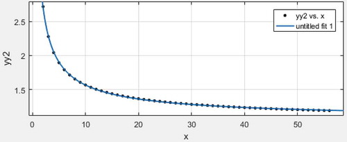
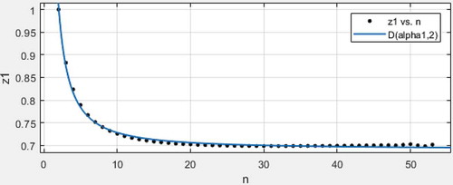
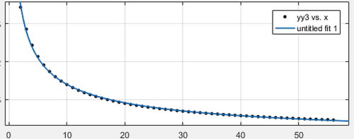
Let $\alpha =1$, here is the variance comparison of three local minimum variance unbiased estimators of expectation and variance when sample size is 2 to 56.

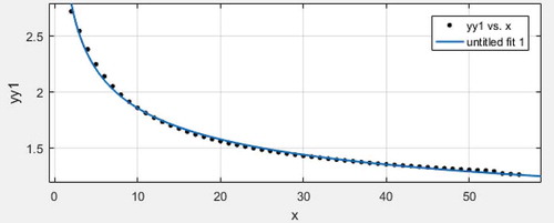
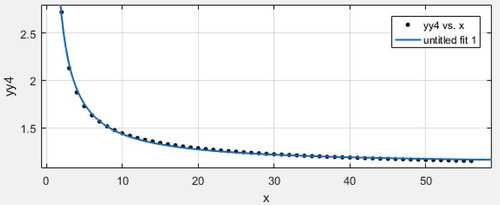
Scatter plot with regression line 1: $e^{\frac{D{\hat{\alpha }}_0}{D{\hat{\alpha }}_1}}=a_1\ast n^{b_1}+c_1,{\hat{a}}_1=2.939,{\hat{b}}_1=-0.3144,{\hat{c}}_1=0.4314$

Scatter plot with regression line2: $e^{\frac{D{\hat{\alpha }}_0}{D{\hat{\alpha }}_2}}=a_2\ast n^{b_2}+c_2,{\hat{a}}_1=2.733,{\hat{b}}_2=-0.7192,{\hat{c}}_2=1.045$

Scatter plot with regression line3: $e^{\frac{D{\hat{\alpha }}_1}{D{\hat{\alpha }}_2}}=a\ast n^b+c,a=0.7955,b=-1.338,c=0.6916$

Comment 5.1. If $X\sim E(\alpha )$, $X_1,...,X_n$ is the sample from $X\sim E(\alpha )$ with sample size$n$, $X_{(1)},...,X_{(n)}$ are the order statistics, then the efficiency comparison of three local minimum variance unbiased estimator of expectation is that: $D{\hat{\alpha }}_0<D{\hat{\alpha }}_1<D{\hat{\alpha }}_2$.

Proof. Because ${\hat{\alpha }}_0=\bar{X}$ is the UMVUE of the expectation, we have $D{\hat{\alpha }}_0<D{\hat{\alpha }}_1$,$D{\hat{\alpha }}_0<D{\hat{\alpha }}_2$. Based on comparison among scatter plot with regression lines 1 or 2 as well as 3, we can obtain $D{\hat{\alpha }}_1<D{\hat{\alpha }}_2$. Hence, $D{\hat{\alpha }}_0<D{\hat{\alpha }}_1<D{\hat{\alpha }}_2$.

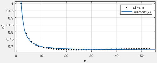
Scatter plot with regression line4: $e^{\frac{D{\hat{\lambda }}_0}{D{\hat{\lambda }}_1}}=a_3\ast n^{b_3}+c_3,{\hat{a}}_3=2.665,{\hat{b}}_3=-0.5197,{\hat{c}}_3=0.8951$

Scatter plot with regression line5: $e^{\frac{D{\hat{\lambda }}_0}{D{\hat{\lambda }}_2}}=a_4\ast n^{b_4}+c_4,{\hat{a}}_4=3.089,{\hat{b}}_4=-0.971,{\hat{c}}_4=1.104$

Scatter plot with regression line6: $e^{\frac{D{\hat{\lambda }}_1}{D{\hat{\lambda }}_2}}=a\ast n^b+c,a=1.02,b=-1.614,c=0.6719$

Comment 5.2. If $X\sim E(\sqrt{\lambda })$, $X_1,...,X_n$ is the sample from $X\sim E(\sqrt{\lambda })$ with sample size$n$, $X_{(1)},...,X_{(n)}$ are the order statistics, then the efficiency comparison of three local minimum variance unbiased estimator of variance is that: $D{\hat{\lambda }}_0<D{\hat{\lambda }}_1<D{\hat{\lambda }}_2$.

Proof. Based on comparison among scatter plot with regression line 4 or 5 as well as 6, we can obtain$D{\hat{\lambda }}_0<D{\hat{\lambda }}_1<D{\hat{\lambda }}_2$.

6. Discussion and conclusion

This article continues the works of references, to improve and perfect the sampling theorem of the exponential distribution. As natural corollary of the sampling theorem of the exponential distribution, one can obtain three local minimum variance unbiased estimators of mean and variance of the exponential distribution, respectively. We know that the sample mean is the UMVUE of expectation and $\frac{n}{1+n}{\bar{X}}^2$ is the UMVUE of variance. Therefore, three local minimum variance unbiased estimators of mean and variance are not substituted for uniformly minimum variance unbiased estimators of mean and variance, respectively, but only rich in natural estimators. From Tables 1–2 and scatter plots with regression lines 1–6, we can draw a conclusion that $D{\hat{\alpha }}_i(i=0,1,2)$ and $D{\hat{\lambda }}_i(i=0,1,2)$ are strictly monotonous decreasing as $n$increases; moreover, they are all convergent to zero, hence, they are all consistent.

Table 1. Variance comparison of three local minimum variance unbiased estimators of expectation under small sample

$n$	$2$	$3$	$4$	$5$	$6$
$D{\hat{\alpha }}_0$	$0.5$	$0.3333$	$0.25$	$0.2$	$0.1667$
$D{\hat{\alpha }}_1$	$0.5$	$0.3572$	$0.2883$	$0.2470$	$0.2192$
$D{\hat{\alpha }}_2$	$0.5$	$0.4048$	$0.3500$	$0.3130$	$0.2858$
$\cdot \cdot \cdot \cdot \cdot \cdot$	$46$	$47$	$48$	$49$	$50$	$\cdot \cdot \cdot \cdot \cdot \cdot$
$\cdot \cdot \cdot \cdot \cdot \cdot$	$0.0217$	$0.0213$	$0.0208$	$0.0204$	$0.0200$	$\cdot \cdot \cdot \cdot \cdot \cdot$
$\cdot \cdot \cdot \cdot \cdot \cdot$	$0.0775$	$0.0768$	$0.0761$	$0.0756$	$0.0751$	$\cdot \cdot \cdot \cdot \cdot \cdot$
$\cdot \cdot \cdot \cdot \cdot \cdot$	$0.1107$	$0.1097$	$0.1087$	$0.1078$	$0.1069$	$\cdot \cdot \cdot \cdot \cdot \cdot$

Table 2. Variance comparison of three local minimum variance unbiased estimators of variance under small sample

$n$		$2$		$3$		$4$		$5$		$6$
$D{\hat{\lambda }}_0$		$2.5$		$1.5909$		$1.1538$		$0.9016$		$0.7386$
$D{\hat{\lambda }}_1$		$2.5$		$1.7932$		$1.4490$		$1.2415$		$1.1010$
$D{\hat{\lambda }}_2$		$2.5$		$2.1063$		$1.8391$		$1.6487$		$1.5407$
$\cdot \cdot \cdot \cdot \cdot \cdot$	$46$		$47$		$48$		$49$		$50$		$\cdot \cdot \cdot \cdot \cdot \cdot$
$\cdot \cdot \cdot \cdot \cdot \cdot$	$0.0883$		$0.0864$		$0.0845$		$0.0828$		$0.0811$		$\cdot \cdot \cdot \cdot \cdot \cdot$
$\cdot \cdot \cdot \cdot \cdot \cdot$	$0.3783$		$0.3748$		$0.3714$		$0.3682$		$0.3751$		$\cdot \cdot \cdot \cdot \cdot \cdot$
$\cdot \cdot \cdot \cdot \cdot \cdot$	$0.5573$		$0.5520$		$0.5468$		$0.5418$		$0.5369$		$\cdot \cdot \cdot \cdot \cdot \cdot$

Remark 6.1. The advantages of those estimators are as follows: If sample is not complete or the record value of the sample mean is not given, and the record value of the difference between sample maximum and mean and the sample minimum are known, then the local minimum variance unbiased estimator of expectation, which is based on $X_{(1)}$ and $(X_{(n)}-\bar{X})$ is a practical estimator; similarly, if sample is not complete or the record value of the sample mean is not given, and the record value of the sample maximum and the sample minimum are known, then the local minimum variance unbiased estimator of expectation, which is based on $X_{(1)}$ and $(X_{(n)}-X_{(1)})$ is a recommendable estimator. If sample is not complete or the record value of the sample mean is not given, and the record value of $(\bar{X}-X_{(1)}{)}^2$and$(X_{(1)}{)}^2$ are known, then the local minimum variance unbiased estimator of variance, which is based on $(X_{(1)}{)}^2$ and $(\bar{X}-X_{(1)}{)}^2$is a practical estimator, similarly, under different sample condition, If sample is not complete or the record value of the sample mean is not given, and the record value of $(X_{(n)}-\bar{X}{)}^2$and $(X_{(1)}{)}^2$are known, or the record value of $(X_{(n)}-X_{(1)}{)}^2$and $(X_{(1)}{)}^2$are known, then the local minimum variance unbiased estimator of variance, which is based on $(X_{(n)}-\bar{X}{)}^2$and $(X_{(1)}{)}^2$or which is based on $(X_{(n)}-X_{(1)}{)}^2$ and $(X_{(1)}{)}^2$is a recommendable estimator, respectively.

Additional information

Funding

The authors received no direct funding for this research.

Notes on contributors

Muzhen Li

Guoan Li is an associate professor in Ningbo University, the Department of Financial Engineering, with more than 70 publications. His research interest includes prediction of earthquake hazards with application to actuarial science, parameter estimation of mixed generalized uniform distribution and its application to data science, multivariate statistical analysis and its application, statistical inferences of multivariate survival distribution under dependent samples, reasonable price assessment of land and real estate acquisition compensation.

References

- Al-Saleh, M. F., & Al-Hadhrami, S. A. (2003). Estimation of the mean of the exponential distribution using moving extremes ranked set sampling. Statistical Papers, 44, 367–382. doi:10.1007/s00362-003-0161-z
- Arnold, B. C. (1968). Parameter estimation for a multivariate exponential distribution. Journal of American Statistical Association, 63, 848–852.
- Baklizi, A., & Dayyeh, W. A. (2003). Shrinkage estimation of P(Y<X)in the exponential case. Communications in Statistics - Simulation and Computation, 32(1), 31–42.
- Cohen, A. C., & Helm, E. R. (1973). Estimation in the exponential distribution. Technometrics, 15(2), 415–418. doi:10.1080/00401706.1973.10489054
- Dixit, U. J., & Nasiri, P. N. (2008). Estimation of parameters of a right truncated exponential distribution. Statistical Papers, 49, 225–236. doi:10.1007/s00362-006-0008-5
- Guoan, L., Jianfeng, L., & Lihong, W. (2017). Parameter estimation for the multivariate exponential distribution which has a location parameter under censored samples or complete samples. Journal of Systems Science & Mathematical Sciences, 37(8), 1854–1865. (in Chinese) Research field.
- Gupta, R. D., & Kundu, D. 0000. Generalized exponential distributions. Australian and New Zealand. doi:10.1111/1467-842X.00072
- Kundu, D., & Gupta, R. D. (2009). Bivariate generalized exponential distributions. Journal of Multivariate Analysis, 100, 581–593. doi:10.1016/j.jmva.2008.06.012
- Lawrance, A. J., & Lewis, P. A. W. (1983). Simple dependent pairs of exponential and uniform random variables. Operations Research, 31, 1179–1197. doi:10.1287/opre.31.6.1179
- Li, G. A. (2016). Sampling fundamental theorem for exponential distribution with application to parameter estimation in the four-parameter bivariate exponential distribution of Marshall and Olkin. Statistical Research, 33(7), 98–102. (inChinese).
- Marshall, A. W., & Olkin, I. (1967). A multivariate exponential distribution. Journal of American Statistical Association, 62(1), 30–44. doi:10.1080/01621459.1967.10482885
- Nie, K., Sinha, B. K., & Hedayat, A. S. (2017). Unbiased estimation of reliability function from a mixture of two exponential distributions based on a single observation. Statistics and Probability Letters, 127, 7–13. doi:10.1016/j.spl.2017.03.026