
 ?Mathematical formulae have been encoded as MathML and are displayed in this HTML version using MathJax in order to improve their display. Uncheck the box to turn MathJax off. This feature requires Javascript. Click on a formula to zoom.
Abstract
Generally, the infection process of most vector-borne diseases involves a latent period in both human hosts and vectors. With regards to other publications, Tian and Song have recently proposed an SIR-SI model to analyze the effects of the incubation period on a vector-borne disease with nonlinear transmission rate. But they were silent on the fact that the partially immune individuals are slightly infective to mosquitoes. So, by considering that the partially immune individuals remain slightly infective to mosquitoes, a similar work has been done in this paper for malaria global transmission dynamics following an SIRS-SI pattern. The basic reproduction ratio has been calculated using the next-generation matrix method. Furthermore, using the characteristic equations and inequality analytical techniques, conditions are given under which the system exhibits threshold behavior as follows: when R0 < 1, the disease-free equilibrium is globally asymptotically stable meaning that the disease will eventually die out; and the unique endemic equilibrium is globally asymptotically stable when R0 > 1 meaning that the disease will persist. Finally, some numerical simulations have been performed to illustrate our theoretical results.
PUBLIC INTEREST STATEMENT
Malaria is one of the reemerging diseases which still remains a major public health issue in several low-income countries around the world. Although mathematical models are an abstract simplification of reality, they can be used to describe or predict the outcomes of epidemics or pandemics providing information that is crucial in informing public health policymakers. This allows them to optimize the use of their limited resources. Otherwise, the last few decades have witnessed an increase of importance of applying equations with distributed delay for understanding real-world phenomena. Therefore, by using delay differential equations, we provide in this paper a further understanding of the impact of incubation period and the role of partially immune individuals in the malaria transmission dynamics and its lasting negative effects. The paper covers a large information on mathematical models of malaria and provides interesting reading due to the original approach and the rich contents.
1. Introduction
Malaria is a vector-borne disease that has been a major public health issue. It is caused by different species of the Plasmodium parasite; the most common being Plasmodium falciparum. The disease is widespread in the tropical and subtropical regions that exist in a broad band around the equator. This includes much of Sub-Saharan Africa, Asia, and Latin America. In 2016, there were 216 million cases of malaria worldwide resulting in an estimated 731 thousand deaths. Approximately 90% of both cases and deaths occurred in Africa. Rates of the disease have decreased from 2000 to 2015 by 37%, but increased from 2014 during which there were 198 million cases. Malaria is commonly associated with poverty and has a major negative effect on economic development. In Africa, it is estimated to result in losses of billion dollars a year due to increased health-care costs, lost ability to work, and negative effects on tourism (Beretta & Kuang, Citation2002; Blyuss & Kyrychko, Citation2014; Traoré, Sangaré, & Traoré, Citation2018).
Mathematical models can project how infectious diseases progress to show the likely outcome of an epidemic and help inform public health interventions. Models use some basic assumptions and mathematics to find parameters for various infectious diseases and use those parameters to calculate the effects of possible interventions, like mass vaccination or drugs distribution programs. The standard technique for developing mathematical descriptions of infectious diseases is to model the system as a set of autonomous ordinary differential Equations (Birkhoff & Rota, Citation1982; Cheng, Wang, & Yang, Citation2012; Jordan & Smith, Citation2004; Ouedraogo, Ouedraogo, & Sangaré, Citation2018). This is an immensely powerful approach which has led to many insights into the factors that affect prevalence and control most of the emerging infectious diseases as dengue, malaria, chikungunya, yellow fever, zika virus, etc. (Diekmann, Getto, & Gyllenberg, Citation2008; Kermack & McKermack, Citation1927; Koutou, Traoré, & Sangaré, Citation2018; Olaniyi & Obabiyi, Citation2013).
The first mathematical model for understanding malaria transmission has been developed by Ross (Koutou et al., Citation2018; Moulay, Aziz-Alaoui, & Cadivel, Citation2011). The Ross’s model consists of two nonlinear differential equations in two state variables that correspond to the proportions of infected human beings and the infected mosquitoes. Macdonald (Citation1957) improved Ross’s more famous differential equations model with some biological assumptions and entomological field data. Since then, multiple models have been done for malaria by several authors. For instance, Aron and May (Chitnis, Hyman, & Cushing, Citation2008; Khan, Khan, & Islam, Citation2015; Traoré et al., Citation2018) added various features of malaria to the model of Macdonald, such as an incubation period in the mosquito, super-infection and a period of immunity in human beings. Besides, the inclusion of acquired immunity proposed by (Chitnis, Cushing, & Hyman, Citation2006; Ruan, Xiao, & Beier, Citation2008) was a major point of malaria modeling. (Ngwa & Shu, Citation2000) proposed a model for malaria transmission in which human hosts follow an SEIRS-like pattern, and vector hosts follow the SEI pattern due to their short life cycle. Moreover, Chitnis et al.(Citation2008) extended the model of Ngwa and Shu by assuming that although individuals in the recovered class are immune, in the sense that they do not suffer from serious illness and do not contract clinical malaria, they still have low levels of Plasmodium in their bloodstream and can infect the susceptible mosquitoes (Bai, Citation2015; Macdonald, Citation1957; Ngwa & Shu, Citation2000; Traoré, Sangaré, & Traoré, Citation2017).
However, many other aspects have aroused much attention and interest in recent decades such as the climate effects on the dynamics of the vector population and the biting rate from mosquitoes to humans (Khan et al., Citation2015; Zhang, Jia, & Song, Citation2014), the stage structure of the vector (Koutou et al., Citation2018; Moulay et al., Citation2011; Traoré et al., Citation2017), the incubation period in the hosts (Diekmann et al., Citation2008; Khan et al., Citation2015) and the form of incidence function. For instance, Traoré et al. (Citation2018) and Koutou et al. (Citation2018) have presented a nonautonomous model and an autonomous model for malaria transmission including the immature stages of the mosquitoes, respectively. Indeed, during the propagation of the epidemic, time delays exist because an individual may not be infectious until some time after becoming infected (Beretta & Kuang, Citation2002; Zhang et al., Citation2014). Some time is required before the infective organism develops in the vector to the level that is sufficient to pass the infection further (Khan et al., Citation2015; Posny & Wang, Citation2014; Van Den Driessche, Citation1996). When we consider the influence of delay on disease spreading, the models take a form of delay differential Equations (Diekmann & Gyllenberg, Citation2012; Kuang, Citation1993; Saker, Citation2010). There are many forms of delays among which we have the concentrated delay, the discrete delay, and the distributed delay. Generally, time delay is assumed to be a single-value. As it is well-known, a constant delay may be applied if the movement time is precisely known, which is not very realistic for a physical situation. In nature, it is obvious that the process depending on the past does not depend on the exact time . But the dependence is somehow distributed. Besides, the length of the latent period varies from disease to disease. For example, according to Anderson and May (Khan et al., Citation2015), measles virus has an infectious period of
days, and influenza has only
days latent period, besides Acquired Immune Deficiency Syndrome (AIDS) has an incubation time ranging from a few months to years after the patient has been shown to get antibodies to the human immunodeficiency virus (HIV) (Omondi, Mbogo, & Luboobi, Citation2018; Wang, Cao, Alsaedi, & Ahmad, Citation2017). Accordingly, equations with distributed delay provide a more flexible and realistic description for real-world phenomena.
In the existing literatures, there exist several works about delay differential equations for infectious diseases especially malaria (Li, Shuai, & Wang, Citation2010; Nakata, Enatsu, & Muroya, Citation2011; Yang & Xiao, Citation2010), to name a few. In (Zhang et al., Citation2014), considering the intracellular delay between initial infection of a cell biting by an infected female anopheles mosquito and the release of new virus particles, Zhang et al. (Citation2014) have proposed and analyzed a non-autonomous SI-SIRS model of malaria global transmission dynamics with distributed time delay. Otherwise, Tian and Song (Citation2017) have more recently constructed and studied a model of a vector-borne disease with two delays and nonlinear transmission rate as follows:
where ,
,
and
,
,
,
,
denote, respectively, the susceptible mosquitoes, the infectious mosquitoes, the susceptible humans, the infectious humans, and the partially immune individuals.
Indeed, malaria differs from many other vector-borne diseases because for it, the partially immune individuals remain slightly infectious to the susceptible mosquitoes (Chiyaka, Tchuenche, Garira, & Dube, Citation2008). Even though they do not show symptoms of malaria, they are still reservoirs of parasites. However, due to their size in an endemic area, their role in the disease transmission cannot be neglected. But both of the previous studies firstly proposed by Zhang et al. (Citation2014) and recently by Tian and Song (Citation2017), respectively, failed to mention this aspect. Motivated by all these works and more precisely by system (1), we have proposed an autonomous SIRS-SI epidemic model to describe malaria transmission dynamics with a wide class of incidence rates and distributed delay. We have then extended the study proposed in (Tian & Song, Citation2017) to malaria including a specific biological assumption that partially immune individuals are infective to susceptible mosquitoes.
The remaining part of the paper is organized as follows. Section 2 concerns the model formulation. In this Section, we have also presented some useful preliminaries and assumptions for the mathematical analysis of the model. In Section 3, we have derived some results about the basic reproduction number, the disease-free equilibrium, and the endemic equilibrium. The global stability of the disease-free equilibrium and the endemic equilibrium were, respectively, studied in Section 4 and 5. Section 6 is devoted to the numerical simulations. Section 7 concludes the paper with some remarks.
2. Model formulation and preliminaries
2.1. Model formulation
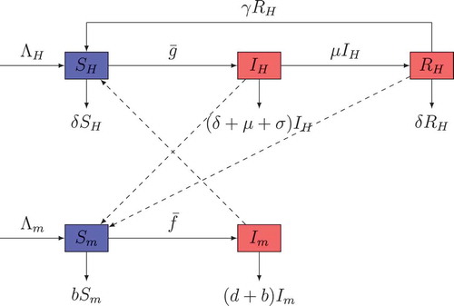
In this part, we formulate a model of malaria spread dynamics relying on some biological aspects. The first compartmental model for malaria transmission has been proposed by Ross. Since many other types of models have been constructed by several authors. Among these types of models, we have the SIRS-SI one that is used in this study. In that model, the human hosts are supposed to follow SIRS and the vector hosts follow SI. The flow between the different compartments is shown by the chart of Figure . For humans, the three compartments represent the total population of humans at a given time , who are susceptible
, infectious
and partially immune
. At the infectious stage, a host may die from the disease or may recover with acquired partial immunity. Partially immune hosts still have protective antibodies and other immune effectors at low levels (Chiyaka et al., Citation2008; Dietz, Molineaux, & Thomas, Citation1974; Macdonald, Citation1957). For mosquitoes, the two compartments represent susceptible mosquitoes
and infectious mosquitoes
at a given time
. Infectious mosquitoes are those that have sporozoites in their salivary glands and can infect the human hosts. Due to the mosquito’s short life cycle, it cannot be recovered from the infection.
Figure 1. The dashed arrows indicate the direction of the infection and the solid arrows represent the transition from one class to another.
From the above descriptions, the total sizes of human population and vector population
are given by
and
respectively.
Functions and
denote the incidence functions and the constant values
,
,
,
,
,
,
,
and
are the model parameters and can be described as follows:
is the natural death rate of the mosquito population,
The disease transmission dynamic is described through the flowchart in Figure . The mathematical model is the following system of delay differential equations
The constant represents the superior limit of incubation times. The incubation period distribution is
, and denotes the fraction of the hosts in which the time taken to become infectious is
. It is assumed to be continuous on
satisfying
and
for
.
Remark 2.1. The two incidence functions and
explain the contact between two species: humans and mosquitoes (Diekmann & Gyllenberg, Citation2012).
2.2. Preliminaries
In this section, we introduce some initial conditions for system (4) as follows:
For any ,
where such as
for all
.
denotes the Banach space
of continuous functions mapping the interval
into
is equipped with the sup norm:
.
For a biological meaning Zhang et al. (Citation2014) we suppose that, for all
, and we consider system (4) in the phase space
. It is clear that all solutions of (4) in
with initial conditions given by (5), remain non-negative.
In the special case, when only discrete experimental data of the past have influence on the present rate of change of the state, the corresponding mathematical equations can be either retarded or neutral differential-difference equations (RDDE or NDDE, respectively). However, the implementation of the complex-step method and the MatLab solver DDE23 are appropriate to compute sensitivities for delay differential equations that have discontinuities in their history functions. This provides a very good approximation of sensitivities as long as discontinuities in the initial data do not cause loss of smoothness in the solution (Bellman & Cooke, Citation1963; Tian & Song, Citation2017).
The incidence rates and
are non-negative differentiable functions on the non-negative quadrant. Furthermore,
and
are positive if and only if both arguments are positive. Note also that when there is no one infected in the human population and the mosquito population, then the incidence functions are equal to zero.
To make biological sense, we assume that the incidence functions and
satisfy the following conditions for all
and
:
(H1)
(H2)
(H3)
The conditions in assumption (H1) state that the infection occurs when there is contact between infected mosquitoes and susceptible humans and also between susceptible mosquitoes and infected or partially immune humans. The assumption (H2) ensures that the model has a unique disease-free equilibrium; and (H3) means that the rate of new infection increases both with not only the infected population size, but also with partially immune individuals (Posny & Wang, Citation2014).
Theorem 2.1. (Bony, Citation1969) Let be a differentiable function and let
be a vector field. Let
and let
be such that
for all
. If
for all
then, the set
is positively invariant.
Lemma 2.1. For any initial conditions given in (5), system (4) admits a unique positive solution for
. Furthermore,
Proof. Note that the right hand side of (4) is completely continuous and locally Lipschitzian on . So, from (Hale, Citation1977; Kuang, Citation1993) we deduce that the solution
of (4) exists and is unique on
, where
represents the maximal time.
Let . We will prove that the set
is positively invariant. Then, let
.
is differentiable and
for all
.
The vector field on the set is given by
Then, ; this proves that the set
is positively invariant. Similarly, we prove that the sets
,
,
,
are positively invariant. So,
is positively invariant.
However, adding the first two equations and adding the last three equations of system (4), we, respectively, obtain
Since , it follows that
Hence, using the differential inequality theorem given in (Birkhoff & Rota, Citation1982), it follows that
Thus,
and
Furthermore, model (4) is mathematically and biologically well-defined in the following set
Thanks to Lemma 2.1, system (4) has the following limit system for any ,
,
, (Nakata et al., Citation2011)
The limit system (12) (see Theorem 3.1 in (Beretta & Takeuchi, Citation1995)) is derived by using the relations
and
3. The model equilibria and the basic reproduction number
3.1. The disease-free equilibrium
Theorem 3.1. Model (4) admits two disease-free equilibria and
respectively given by
and
Proof. On the one hand when we set all the infected classes to zero, the following equations yield and
. We then obtain the second infection-free equilibrium point
.
□
On the other hand, setting the susceptible mosquitoes class to zero, we deduce the first infection-free equilibrium point .
Remark 3.1. The disease-free equilibrium represents the case where there is no disease and the area is completely devoid of mosquitoes.
The disease-free equilibrium represents the case where the mosquito population exists but there is no malaria.
The first case is difficult to obtain in most areas where malaria is intensive because of the difficulties and the environmental effects due to the complete eradication of the mosquito population. Hence, in this paper, we focus our study on the last one because it is more biologically realistic (Traoré et al., Citation2018).
3.2. The basic reproduction number
The basic reproduction number is now unanimously recognized as a key concept in mathematical epidemiology. It is commonly denoted by and represents the average number of new infections produced directly and indirectly by a single infective individual, when that individual is introduced into a completely susceptible population during the infective period. For about 20 years,
has been part of the majority of research articles using mathematical modeling. For classical epidemic models, it is common that the basic reproduction number is a threshold in the sense that, when it is less than unity, on average each infected individual infects fewer than one individual, and the disease dies out. If
, on average, each infected individual infects more than one other individual, so we would expect the disease to spread (Van den Driessche, Citation1996; Van den Driessche & Watmough, Citation2002).
In fact, new infections occur during contacts between susceptible individuals and infectious individuals. Here, only the following three classes ,
and
are considered to be disease states. Therefore, using the technique described in (Van den Driessche & Watmough, Citation2002), we compute the basic reproduction number as follows.
Linearizing the infected equations of system (4) at disease-free equilibrium , we obtain the following system:
where the matrices and
are given by
and
The matrix is called the next-generation operator, and it is known that the basic reproduction is
. For system (4), it is given by
From above, it is obvious that the basic reproduction number varies directly to the number of partially immune individuals who remain infective to mosquito population.
3.3. The endemic equilibrium
Note that the delay systems and the ordinary differential equation systems share the same equilibria (Beretta & Kuang, Citation2002; Yang & Xiao, Citation2010).
Lemma 3.1. If , there exists a unique positive solution
of model (4) with initial conditions (5) satisfying to the following system
Proof. At a fixed point e the incidence functions and the constant valu
From the last equation of the system we obtain
Adding the first two equations of (19), we obtain that
Moreover, adding the third and the fourth equations of (19), it then follows that
Let us consider the following function
with
and
We can see that the function is continuous and
.
Any zero of
is in the set
where and
correspond to endemic equilibrium components.
Moreover,
and then, in order to have a solution to the equation
on the set
the function must be increasing at
.
Positing leads to the following condition
It follows that
and
Hence,
and
Adding the inequalities (25) and (26), we observe that the condition is equivalent to
. □
4. The local stability of equilibria
In this section, we study the local stability of our model equilibria.
Theorem 4.1. If , and the assumption (H2) holds, then the disease-free equilibrium
is locally asymptotically stable.
Proof. We begin by linearizing Equation (4) at , with
and
.
From hypothesis (H2), we have for all positive ,
and then
Moreover, for all positive , the following condition yields
and consequently,
The linearization of system (4) at the disease-free equilibrium is given by
Here, we apply the principle of linearized stability method established in (Diekmann et al., Citation2008; Diekmann & Gyllenberg, Citation2012).
Looking as in (Blyuss & Kyrychko, Citation2014; McCluskey, Citation2010), the solution of the following form,
where and
.
Therefore, plugging the relation (28) into (27) and canceling from each term, yields the following matrix equation:
with the next-generation matrix given by
There exist non-zero solutions if and only if . Thus, we obtain the characteristic equation as follows:
Consider the quantities and
defined by
Then,
and so, cannot be the solution of (31). Hence, all characteristic roots have a negative real part, and therefore
is locally asymptotically stable. □
Suppose that the incidence functions and
satisfy the following conditions at endemic equilibrium
(H4)
(H5)
Theorem 4.2. If , (H4) and (H5) hold, then the endemic equilibrium is locally asymptotically stable.
Proof. The condition guaranteeing the existence of an endemic equilibrium
with
and
.
The linearization of system (4) about the endemic equilibrium is given by
We demonstrate that all the roots of the characteristic equation have a negative real part. So, as in the previous proof, using Equation (28) into (34) and canceling from each term and rearranging the following matrix equation yields
with
There exist non-zero solutions if and only if . Hence, we obtain the characteristic equation as follows:
Consider the following quantities
Hence, thanks to the hypothesis (H4) and (H5),
and so the characteristic Equation (37) has solutions with negative real part. In fact, the characteristic Equation (37) has solutions with non-negative real part if and only if all of the above inequalities are equations. Thus, the endemic equilibrium
is locally asymptotically stable.
Now, let us analyze the global behavior of the equilibria.
5. The global stability of the equilibria
In this section, we study the global behavior of the endemic equilibrium. First, let us make the following useful assumptions:
(H6) For all ,
and
Theorem 5.1. The disease-free equilibrium is globally asymptotically stable in
whenever
.
Proof. The proof is based on using a comparison theorem (Lakshmikantham, Leela, & Martynyuk, Citation1989). Note that the equations of the infected components in system (4) can be expressed as in (Posny & Wang, Citation2014) like
where the matrixes and
are respectively given by (15) and (16).
Using the fact that all the eigenvalues of the matrix have negative real parts, it follows that the linearized differential inequality system (40) is stable whenever
. Indeed, we can see that all eigenvalues of the matrix
satisfy Equation (31). By the same reasoning as the proof of the Theorem 4.1, we deduce that the eigenvalues of the matrix
have negative real parts since
, (Van den Driessche & Watmough, Citation2002; Yang & Xiao, Citation2010).
Thus, as
for system (40). Consequently, by the standard comparison theorem (Lakshmikantham et al., Citation1989),
as
and substituting
into system (4) we obtain
and
as
.
So, as
for
. Therefore, the disease-free equilibrium
is globally asymptotically stable. ◴
Let us consider as in (Nakata et al., Citation2011), the positive function, for all
and the following region
Theorem 5.2. If , then the endemic equilibrium
is globally asymptotically stable in
.
Proof. Let us consider the following Lyapunov function
with
where ,
,
, and
are respectively defined as follows
and
Now, let us show that .
First, we calculate as:
Substituting by its expression from the third equation of system (4) and also
it then follows that
We will use the following notations if need be
and so can be rewritten as
Secondly, we calculate . Indeed,
At endemic equilibrium, thanks to the fourth equation of the system (4), we obtain that
Thus,
Using the above notations given by (44), it follows that
The above notations given by (44) lead to the following equations
In addition,
Consequently,
And then,
Besides, we have
Let us calculate now .
At endemic equilibrium point, we have
and
Hence,
In summary, all these calculations lead to the following result,
Secondly, we calculate . As previously, let us begin by calculating
.
For the sake of simplicity, we adopt the following notations
At the endemic state, from the first equation of system (4), we have
Hence
Now, let us calculate
At endemic equilibrium, thanks to the second equation of system (4), the following equality yields
Consequently,
Moreover, as from above, we show that
And so,
In conclusion, thanks to the inequalities (45) and (47), we then have . Thus, thanks to the LaSalle’s invariance principle (Koutou et al., Citation2018; Moulay et al., Citation2011), the endemic equilibrium is globally asymptotically stable. □
6. Numerical simulations
In this section, we use numerical tools to illustrate the theoretical results obtained in earlier sections for our model. For that, we consider as in (Nakata et al., Citation2011), the following corresponding discrete delay model of (4)
It is easy to see that (48) also has the same endemic equilibrium of (4) if and only if the condition holds (Nakata et al., Citation2011). Moreover, in this computation, the functions
and
are chosen as follows
and
.
Figures – show the numerical simulations of model (4), with different values of the model parameters given in the corresponding captions, with the following initial conditions ,
,
,
,
.
Figure 2. Density of infected mosquitoes and infected humans when, ,
,
,
,
,
,
,
,
,
and
and
respectively for the sub-figures (a) and (b).
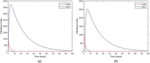
Figure 3. Periodic solutions with delay and
,
,
,
,
,
,
,
,
,
.
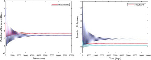
Figure 4. Periodic solutions with a length incubation period and
,
,
,
,
,
,
,
,
,
.
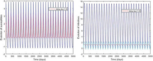
Figure 5. Density of infected mosquitoes versus susceptible mosquitoes; and susceptible mosquitoes versus infected mosquitoes when and
,
,
,
,
,
,
,
,
,
.
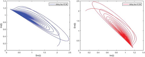
Figure 6. Density of infected humans versus susceptible humans; and susceptible humans versus partially immune individuals when and
,
,
,
,
,
,
,
,
,
.
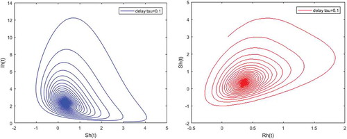
Figure 7. Density of partially immune individuals versus susceptible; and infected humans versus partially immune individuals when and
,
,
,
,
,
,
,
,
,
.
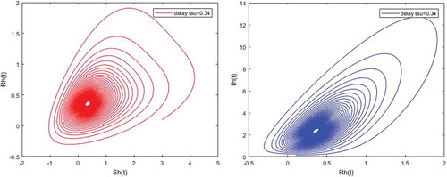
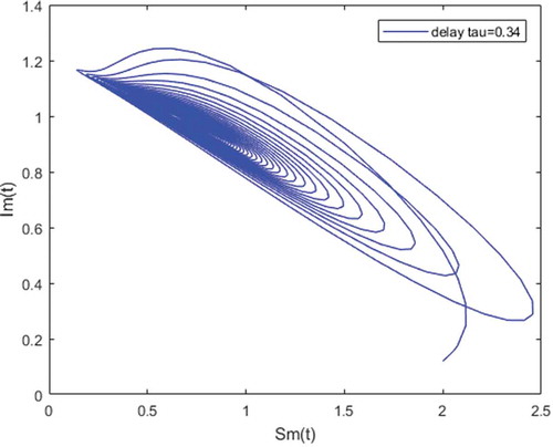
Figure 8. Limit cycles appearance when and
,
,
,
,
,
,
,
,
,
.

Figure shows that the disease-free equilibrium is global asymptotically stable whenever the threshold parameter is less than unity and this, for any value of time-lag. For Figure , the parameter values which are chosen lead to
which is less than unity. This result illustrates our Theorem 4.1. While we observe that the length of the incubation period decreases the number of infectious hosts. For instance, with
there are about
infected mosquitoes and
infected humans (see sub-figure (a)). When we increase the incubation period to
, the number of infected hosts decreases and we obtain about
for mosquitoes and
for humans (see sub-figure (b)).
Figures – illustrate the existence and the global stability of the unique endemic equilibrium of the model. The parameter values which are chosen lead to which is greater than unity. Theorem 4.2 then holds.
However, Figures and show that for some particular values of time-lag , oscillations occur which can destabilize the system, and periodic solutions can arise due to Hopf bifurcation (see Figures and ). Moreover, one biological significance of oscillations is that each peak in the parasite marks a clinical episode of the disease for the host whatever it is (Ncube, Citation2013; Rihan & Anwar, Citation2012). This type of information would be essential for disease control and management strategies.
While Figures – show that a little incubation period such as , the endemic steady of the model is exactly reached. Increasing this value can destabilize the system and give rise to a stable limit cycle. Indeed, the limit cycle is a trajectory for which the dynamics of the system would be constant over a cycle. This means that the epidemic gets a limit progression (Rasmussen, Wake, & Donaldson, Citation2003).
7. Discussions and conclusion
In this paper, we have studied in detail the persistence, the extinction, and the global asymptotic stability of an autonomous malaria transmission model with distributed time delay. The effect of the time-lag parameter on the behavior of the infection has been investigated. We determined the basic reproduction number
of the model and proved that it is not complete without considering the partially immune individual’s effects on the vectors and the malaria infection rate. And, we have shown that it is the threshold dynamics between the persistence and the extinction of the disease. More precisely, we have proven that if
, the disease-free equilibrium is globally asymptotically stable. In this case, the epidemic will be extinct gradually. Similarly, if
, the endemic equilibrium point is globally asymptotically stable. Hence, the disease will persist. Our theoretical studies deliver some new insights for understanding the propagation of the diseases and the information on biological networks, especially malaria.
Finally, a series of numerical simulations have been presented to show that the model agrees with the theoretical results. Furthermore, that numerical simulations show the impact of the delay on the model’s global behavior as follows: a great value of delay slows down the spreading of the disease, while a small value of time delay accelerates it. For particular values of time-lag , oscillations occur which can destabilize the system, and periodic solutions can arise due to Hopf bifurcation. Although the underlying DDE model is simple, it displays very rich dynamics, such as quasi-periodic and chaotic patterns, and is suitable for large population densities (Sekiguchi & Ishiwata, Citation2010; Wang, Zhang, & Liu, Citation2018; Zhang & Teng, Citation2009).
Moreover, it emerges from our study that the incubation period is an important factor in the dynamics of malaria transmission. So, it can be used as a good parameter in fighting against malaria propagation.
Cover Image
Source: Author.
Additional information
Funding
Notes on contributors
Ousmane Koutou
Ousmane Koutou is a vigorous researcher PhD student at University Nazi BONI. His research interests lie in the field of Mathematical Biology and the present paper is a portion of his thesis under the supervision of Dr. Boureima SANGARÉ. He has published a number of research papers in reputed international journals, including, Advance in Difference Equation (Springer) and others journals.
Bakary Traoré
Bakary Traoré is a PhD student at University Nazi BONI under the supervision of Dr. Boureima SANGARÉ. A vigorous researcher in the area of Mathematical modelling, he has presented many papers in conferences and has published a number of research papers in reputed international journals, including Journal of Biological Dynamics (Taylor’s and Francis), Advance in Difference Equation (Springer) and others journals.
Boureima Sangaré
Dr Boureima Sangaré research interests lie in the field of Mathematical Modelling and four PhD students are currently working with him. He has published his research contributions in some internationally renowned journals whose publishers are Springer, Taylor & Francis and other journals.
References
- Bai, Z. (2015). Threshold dynamics of a periodic SIR model with delay in an infected compartment. Mathematical Biosciences & Engineering, 12(3), 555–564. doi:10.3934/mbe.2015.12.555
- Bellman, R., & Cooke, K. L. (1963). Differential-difference equations. New York and London: Academic Press.
- Beretta, E., & Kuang, Y. (2002). Geometric stability switch criteria in delay differential systems with delay dependent parameters. SIAM Journal on Mathematical Analysis, 33(5), 1144–1165. doi:10.1137/S0036141000376086
- Beretta, E., & Takeuchi, Y. (1995). Global stability of an SIR epidemic model with time delays. Journal of Mathematical Biology, 33, 250–260.
- Birkhoff, G., & Rota, G. C. (1982). Ordinary differential equations. Boston: Ginn.
- Blyuss, K. B., & Kyrychko, Y. N. (2014). Instability of disease-free equilibrium in malaria model with immune delay. Mathematical Biosciences, 248, 54–56. doi:10.1016/j.mbs.2013.12.005
- Bony, J. M. (1969). Principe du Maximum, Inégalité de Harnack et Unicité du Probleme de Cauchy Pour les Opérateurs Elliptiques Dégénérés. Annales de L’institut Fourier (Grenoble), 19, 277–304. doi:10.5802/aif.319
- Cheng, Y., Wang, J., & Yang, X. (2012). On the global stability of a generalized cholera epidemiological model. Journal of Biological Dynamics, 6(2), 1088–1104. doi:10.1080/17513758.2012.728635
- Chitnis, N., Cushing, J. M., & Hyman, J. M. (2006). Bifurcation analysis of a mathematical model for malaria transmission. SIAM Journal on Applied Mathematics, 67, 24–25. doi:10.1137/050638941
- Chitnis, N., Hyman, J. M., & Cushing, J. M. (2008). Determining important parameters in the spread of malaria through the sensitivity analysis of a mathematical model. Bulletin of Mathematical Biology, 70(5), 1272–1296. doi:10.1007/s11538-008-9299-0
- Chiyaka, C., Tchuenche, J. M., Garira, W., & Dube, S. (2008). A mathematical analysis of the effects of control strategies on the transmission dynamics of malaria. Applied Mathematics and Computing, 195(3), 641–662.
- Diekmann, O., Getto, P., & Gyllenberg, M. (2008). Stability and bifurcation analysis of volterra functional equations in the light of suns and stars. SIAM Journal on Mathematical Analysis, 39, 1023–1069. doi:10.1137/060659211
- Diekmann, O., & Gyllenberg, M. (2012). Equations with infinite delay: Blending the abstract and the concrete. Journal of Differential Equations, 252, 819–851. doi:10.1016/j.jde.2011.09.038
- Dietz, K., Molineaux, L., & Thomas, A. (1974). A malaria model tested in the african savannah. Bulletin of the World Health Organization, 50, 347–357.
- Hale, J. K. (1977). Theory of functional differential equations. New York: Springer-Verlag.
- Jordan, D. W., & Smith, P. (2004). Nonlinear ordinary differential equations. New York, USA: Oxford University Press.
- Kermack, W. O., & McKermack, A. G. (1927). A contribution to the mathematical theory of epidemics. Proceedings of the Royal Society A: Mathematical, Physical and Engineering Sciences, 115(772), 700–721. doi:10.1098/rspa.1927.0118
- Khan, M. A., Khan, Y., & Islam, S. (2015). Dynamical system of a SEIQV epidemic model with nonlinear generalized incidence rate arising in biology. International Journal of Biomathematics, 10(7), 1750096 (19 pages), Article ID 1550082. doi:10.1142/s1793524517500966
- Koutou, O., Traoré, B., & Sangaré, B. (2018). Mathematical modeling of malaria transmission global dynamics: Taking into account the immature stages of the vectors. Advances in Difference Equations, 2018(220). doi:10.1186/s13662-018-1671-2
- Kuang, Y. (1993). Delay differential equations with applications in population dynamics. Mathematics in Science and Engineering, 191, 398 p. Cambridge: Academic Press.
- Lakshmikantham, V., Leela, S., & Martynyuk, A. A. (1989). Stability analysis of nonlinear systems. New York: Marcel Dekker.
- Li, M. Y., Shuai, Z., & Wang, C. (2010). Global stability of multi-group epidemic models with distributed delays. Journal of Mathematical Analysis and Applications, 361, 38–47. doi:10.1016/j.jmaa.2009.09.017
- Macdonald, G. (1957). The epidemiology and control of malaria (pp. 3, 31, 48, 96). London: Oxford University Press.
- McCluskey, C. C. (2010). Global stability of an SIR epidemic model with delay and general nonlinear incidence. Mathematical Biosciences & Engineering, 7(4), 837–850. doi:10.3934/mbe.2010.7.837
- Moulay, D., Aziz-Alaoui, M. A., & Cadivel, M. (2011). The chikungunya disease: Modeling, vector and transmission global dynamics. Mathematical Biosciences, 229(1), 50–63. doi:10.1016/j.mbs.2010.10.008
- Nakata, Y., Enatsu, Y., & Muroya, Y. (2011). On the global stability of an SIRS epidemic model with distributed delays. Discrete and Continuous Dynamical Systems Supplement, 2011, 1119–1128.
- Ncube, I. (2013). Absolute stability and hopf bifurcation in a plasmodium malaria model incorporating discrete immune response delay. Mathematical Biosciences, 243, 131–135. doi:10.1016/j.mbs.2013.02.010
- Ngwa, G. A., & Shu, W. S. (2000). A mathematical model for endemic malaria with variable human and mosquito populations. Mathematical and Computer Modelling, 32, 747–763. doi:10.1016/S0895-7177(00)00169-2
- Olaniyi, S., & Obabiyi, O. S. (2013). Mathematical model for malaria transmission dynamics in human and mosquito populations with nonlinear forces of infection. International Journal of Pure and Applied Mathematics, 88(1), 125–156. doi:10.12732/ijpam.v88i1.10
- Omondi, E. O., Mbogo, R. W., & Luboobi, L. S. (2018). Mathematical modelling of the impact of testing, treatment and control of the HIV transmission in Kenya. Cogent Mathematics & Statistics, 5, 1–16. doi:10.1080/25742558.2018.1475590
- Ouedraogo, H., Ouedraogo, W., & Sangaré, B. (2018). A self-diffusion mathematical model to describe the toxin effect on the Zooplankton dynamics. Nonlinear Dynamics and Systems Theory, 18(4), 392–408.
- Posny, D., & Wang, J. (2014). Modelling cholera in periodic environments. Journal of Biological Dynamics, 8(1), 1–19. doi:10.1080/17513758.2014.896482
- Rasmussen, H., Wake, G. C., & Donaldson, J. (2003). Analysis of a class distributed delay logistic differential equations. Mathematical and Computer Modelling, 38, 123–132. doi:10.1016/S0895-7177(03)90010-0
- Rihan, F. A., & Anwar, M. N. (2012). Qualitative analysis of delayed SIR epidemic model with a saturated incidence rate. International Journal of Differential Equations, 2012, 13, Article ID 408637.
- Ruan, S., Xiao, D., & Beier, J. C. (2008). On the delayed Ross-Macdonald model for malaria transmission. Bulletin of Mathematical Biology, 70(4), 1098–1114. doi:10.1007/s11538-007-9292-z
- Saker, S. H. (2010). Stability and hopf bifurcations of nonlinear delay malaria epidemic model. Nonlinear Analysis, Real World Applications, 11, 784–799. doi:10.1016/j.nonrwa.2009.01.024
- Sekiguchi, M., & Ishiwata, E. (2010). Global dynamics of a discretized SIRS epidemic model with time delay. Journal of Mathematical Analysis and Applications, 371, 195–202. doi:10.1016/j.jmaa.2010.05.007
- Tian, D., & Song, H. (2017). Global dynamics of a vector-borne disease model with two delays and nonlinear transmission rate. Mathematical Methods in the Applied Sciences, 40(1818), 6411–6423. doi:10.1002/mma.4464
- Traoré, B., Sangaré, B., & Traoré, S. (2017). Mathematical model of malaria transmission with structured vector population and seasonality. Journal of Applied Mathematics, 2017, 15, Article ID 6754097.
- Traoré, B., Sangaré, B., & Traoré, S. (2018). A mathematical model of malaria transmission in a periodic environment. Journal of Biological Dynamics, 12(1), 400–432. doi:10.1080/17513758.2018.1468935
- Van den Driessche, P. (1996). Some epidemiological models with delays. In M. Martelli (Ed.), Differential equations and applications to biology and industry (Claremont, CA, 1994) (pp. 507–520). River Edge, NJ: World Scientific Publishing.
- Van den Driessche, P., & Watmough, J. (2002). Reproduction numbers and sub-threshold endemic equilibria for compartmental models of disease transmission. Mathematical Biosciences, 180, 29–48.
- Wang, L., Zhang, X., & Liu, Z. (2018). An SEIR epidemic model with relapse and general nonlinear incidence rate with application to media impact. Qualitative Theory of Dynamical Systems, 17(2), 309–329. doi:10.1007/s12346-017-0231-6
- Wang, Y., Cao, J., Alsaedi, A., & Ahmad, B. (2017). Edge-based SEIR dynamics with or without infectious force in latent period on random networks. Communications in Nonlinear Science and Numerical Simulation, 45, 35–54. doi:10.1016/j.cnsns.2016.09.014
- Yang, Y., & Xiao, D. (2010). A mathematical model with delays for schistosomiasis. Chinese Annals of Mathematics, 31B(4), 433–446. doi:10.1007/s11401-010-0596-1
- Zhang, T. L., & Teng, Z. D. (2009). Permanence and extinction for a nonautonomous SIRS epidemic model with time delay. Applied Mathematical Modelling, 33(2), 1058–1071. doi:10.1016/j.apm.2007.12.020
- Zhang, X., Jia, J., & Song, X. (2014). Permanence and extinction for a nonautonomous malaria transmission model with distributed time delay. Journal of Applied Mathematics, 2014, 16. ID 139046.