A simple and efficient method for finding the closest generalized lambda distribution to a specific model

Abstract

The four-parameter Generalized Lambda distribution (GLD) can be used to approximate many probability distributions. We present a simple and efficient two-stage process for finding optimal GLD parameters to approximate a specified distribution. The probability density quantile function is first used to find the best GLD shape parameters. Given those shape parameters, it is then straightforward to find the best location and scale parameters. We highlight the excellent performance of our approach with comparisons to two existing and popular methods for a wide choice of distributions. Finally, we show that this is method can be used with other distributions by providing applications also to the Generalized Beta distribution.

Keywords:

• quantile density
• probability density quantiles
• generalized lambda distribution
• generalized beta distribution

PUBLIC INTEREST STATEMENT

The Generalized Lambda distribution (GLD) is a commonly used distribution in many fields, including finance and economics. Due to its flexibility, the GLD is widely used to approximate other distributions. Motivated by this fact, this article presents a new method which can be simply executed to obtain the optimal parameters for the GLD to approximate another distribution. Further, the results are compared with two other methods that are generally used to estimate GLD parameters to show that this new method has favourable qualities.

1. Introduction

Ramberg and Schmeiser (1974) introduced the Generalized Lambda distribution (GLD), a flexible four-parameter family of distributions that can be used to approximate a very large number of probability distributions. It is defined by its quantile function, which depends on a location parameter ${\lambda }_1$, inverse scale parameter ${\lambda }_2$, and shape parameters ${\lambda }_3$ and ${\lambda }_4$. There are several re-parameterizations of the GLD, but the FKML parameterization (Freimer, Kollia, Mudholkar, & Lin, 1988) shown in (1) is simplest to work with, being defined for all real parameter values subject only to ${\lambda }_2>0$. This GLD is used extensively throughout the text by Karian and Dudewicz (2016) regarding fitting statistical distributions to data and the authors of a book (Pfaff, 2016) on financial risk modeling call this GLD an ideal choice.

Given the correct parameters, the GLD distribution equates to several well-known distributions (e.g. the uniform, exponential, logistic) and for many others, a close approximation is possible (e.g. normal, Cauchy, log-normal). While the use of two or more shape parameters increases the flexibility of generalized distributions such as the GLD, an exhaustive search for optimal parameters becomes difficult due to the dimension over which the search need be carried out. We propose to use the probability density quantile (Staudte, 2017) which depends only on the shape parameters and which is defined on the interval $[0,1]$ making the task of finding optimal shape parameters a simple one. It is then straightforward to find the location and inverse scale parameters. Our investigations to be detailed later reveal excellent performance of this new approach when compared to commonly used methods. Additionally, the method we propose is applicable to other distributions such as the generalized beta distribution which we explore in Section 5. Consequently, researchers exploring new generalized distributions will also find our method useful.

An outline of this paper is as follows: In Section 2 we introduce definitions used throughout. We also work through some simple examples that help to motivate our work. In Section 3 we briefly discuss two existing methods that are commonly used to identify GLD parameters before introducing our procedure. Examples are considered in Section 4, where our method is shown to perform relatively well in identifying optimal GLD parameters. Further, a web application is also provided. We then show in Section 5 that the method is suitable also for fitting generalized beta distributions to a given model. A discussion and further work are proposed in Section 6.

2. Definitions and some motivating examples

In this section we introduce definitions and notation to be used in the sequel.

2.1. Quantile, quantile density and density quantile functions

For $u\in (0,1)$, let $Q(u)=F^{-1}(u)$ denote the quantile function associated with distribution function $F$. Let $f=F^{\prime }$ denote the probability density function and assume $f(x)>0$ for all $x$ in its domain. The quantile density function (Parzen, 1979) is defined as $q(u)=Q^{\mathrm{\prime }}(u)=1/f\left[Q(u)\right]$. It was earlier called the sparsity index by Tukey (1965). The quantile density function is often useful in nonparametric modeling and inference. For example, for $\widehat{Q(u)}=F_n^{-1}(u)$ denoting the estimated pth quantile arising from the empirical distribution function $F_n$ for a simple random sample of $n$ observations, an asymptotic variance for $\widehat{Q(u)}$ is $u(1-u)q^2(u)/n$, e.g. page 52 of Staudte and Sheather (1990). Parzen (1979) called the reciprocal of the quantile density function the density quantile function, and we will denote it here by $f_Q(u)=f[Q(u)].$

2.2. Probability density quantile functions

The probability density quantile, introduced recently by Staudte (2017), is shown to be useful in the study of shape in a location-scale free environment; see also Staudte and Xia (2018).

Definition 2.1 Staudte (2017): For $U\sim \mathrm{U}\mathrm{n}\mathrm{i}\mathrm{f}(0,1)$ and $\kappa =E[f_Q(U)]$ assumed to be finite, the probability density quantile (pdQ) is defined to be $f_Q^{\ast }(u)=f_Q(u)/\kappa$ for $0<u<1$.

The pdQ is defined for all lattice distributions and continuous distributions having square-integrable densities; it is free of location and scale parameters and defined on the finite domain $[0,1]$. Further, it retains information regarding shape such as asymmetry and tail behaviour (Staudte, 2017). It, therefore, can provide a simple means to identify suitable shape parameters. Once we introduce the GLD distribution next, we will provide some simple examples using the pdQ to find shape parameters.

2.3. The generalized lambda distribution

The Generalized Lambda Distribution (GLD) of Freimer et al. (1988) is defined in terms of its quantile function:

(1) $Q(u)={\lambda }_1+\frac{1}{{\lambda }_2}\left[\frac{u^{{\lambda }_3}-1}{{\lambda }_3}-\frac{{(1-u)}^{{\lambda }_4}-1}{{\lambda }_4}\right]$(1)

where ${\lambda }_1$ is a location parameter, $1/{\lambda }_2>0$ a scale parameter and ${\lambda }_3,{\lambda }_4$ are shape parameters.

It is easy to see that the quantile density function for the GLD is $q(u)=Q^{\prime }(u)={\lambda }_2^{-1}\left[u^{{\lambda }_3-1}+{(1-u)}^{{\lambda }_4-1}\right]$ so that the density quantile function is

(2) $f_Q(u)=\frac{{\lambda }_2}{u^{{\lambda }_3-1}+{(1-u)}^{{\lambda }_4-1}}.$(2)

In general, no closed-form solution for the integral $\kappa ={\int }_0^1{f}_Q(u)du$ exists, but it can be evaluated computationally and quite efficiently since integration occurs only between the finite bounds zero and one.

2.4. Some motivating examples

The following examples are used to motivate our approach that follows. While for these examples exact solutions are possible, our method provides a way to determine parameter choices for the GLD to closely approximate the true density when exact solutions are not possible.

2.4.1. The uniform distribution

For a simple motivating example, we consider the Uniform $(a,b)$ distribution with quantile function $Q_1(u)=a+u(b-a)$ and quantile density function $q_1(u)=Q_1^{\prime }(u)=(b-a)$. Of course a simple inspection of the quantile functions for the uniform and GLD distributions reveals that ${\lambda }_1=(a+b)/2$, ${\lambda }_2=2/(b-a)$, ${\lambda }_3=1$ and ${\lambda }_4=1$ results in the Uniform$(0,1)$ distribution. Below we show how the same results can be arrived at via the GLD.

The density quantile function for the uniform is $f_{Q_1}(u)=1/(b-a)$ where ${\int }_0^1{f}_{Q_1}(u)du=1/(b-a)$ leading to the uniform pdQ $f_{Q_1}^{\ast }(u)=1.$ Now by choosing ${\lambda }_3=1$ and ${\lambda }_4=1$ we can assure that the GLD pdQ is also free of $u$, as it is for the uniform distribution. For the GLD distribution $f_Q(u)=\lambda$ and $f_Q^{\ast }(u)=1$ so that for these choices of ${\lambda }_3$ and ${\lambda }_4$ we have equality between the uniform and GLD pdQs.

2.4.2. The exponential distribution

The quantile function for the exponential distribution with rate parameter $\lambda$ is $Q(u)=-log(1-u)/\lambda$. Consequently, the pdQ $f_{Q_1}^{\ast }(u)=2(1-u)$ (see also Staudte, 2017). For the GLD, for ${\lambda }_3=\mathrm{\infty }$ and ${\lambda }_4=0$, $f_Q(u)={\lambda }_2(1-u)$ so that $f_Q^{\ast }(u)=2(1-u)$ which is equal to the pdQ for the exponential. Note that $\underset{{\lambda }_4\to 0}{lim}\left[{(1-u)}^{{\lambda }_4}-1\right]/{\lambda }_4=log(1-u)$ so that the quantile function for the GLD is $Q(u)={\lambda }_1+log(1-u)/{\lambda }_2$ and equality with the exponential quantile function is achieved by choosing ${\lambda }_1=0$ and ${\lambda }_2=\lambda$.

3. Methods

3.1. Existing methods

We start by briefly describing two commonly used methods for obtaining GLD parameters. These methods are available in the bda package (Wang, 2015) available for the R statistical software (R Core Team, 2017) and will be used later to assess our new approach which is also detailed here.

3.1.1. The moments method

Karian and Dudewicz (2003) and Lakhany and Mausser (2000) describe the moments matching method for GLD on the basis of the first four central moments. To estimate the GLD parameters, they match mean, variance, skewness and kurtosis of the GLD with the moments resulting in a system of non-linear equations that can be solved using optimization methods to obtain parameters.

3.1.2. The percentile matching method

Rather than moments, the percentile matching method equates a selected number of percentiles with the GLD theoretical percentiles. By optimizing this set of non-linear equations, parameters can be obtained for the given Generalized Lambda Distribution as discussed by Karian and Dudewicz (1999) and Tarsitano (2005). This method is preferred over the moments method as it applies less weight to the extremes and also could be used in situations where moments do not exist.

3.2. Choosing parameters based on the pdQ

Throughout let $Q$ denote the GLD quantile function given in (1) and let $f_Q^{\ast }$ denote the corresponding GLD pdQ where we write, for a given $u$, $f_Q^{\ast }(u;{\lambda }_3,{\lambda }_4)$ to emphasize that the GLD is a function of the two shape parameters. Further, let $Q_1$ and $f_{Q_1}^{\ast }$ be the quantile function and pdQ for another distribution to be approximated.

3.2.1. Step 1: choosing shape parameters

In the first step, we seek the GLD shape parameters ${\lambda }_3$ and ${\lambda }_4$ that minimizes the expected squared distance between the pdQs $f_Q^{\ast }$ and $f_{Q_1}^{\ast }$ given as

$\underset{{\lambda }_3,{\lambda }_4}{\mathrm{a}\mathrm{r}\mathrm{g}\mathrm{m}\mathrm{i}\mathrm{n}}{\int }_0^1{\left[f_Q^{\ast }(u;{\lambda }_3,{\lambda }_4)-f_{Q_1}^{\ast }(u)\right]}^{2}du.$

While this need not be an onerous task, since the integral needs to be evaluated over the finite bounds 0 to 1, it is simple to approximate this step using a discrete set of $u$s given as ${\left\{u_j=(j-1/2)/J\right\}}_{j=1}^J$ for a positive integer $J$. Further, it may be appropriate to apply less weighting to the extreme tails to ensure that the GLD distribution is close to the distribution to be approximated in regions of high density mass. Therefore, we suggest choosing the optimal shape parameters using

(3) $({\lambda }_3^{\ast },{\lambda }_4^{\ast })=\underset{{\lambda }_3,{\lambda }_4}{\mathrm{a}\mathrm{r}\mathrm{g}\mathrm{m}\mathrm{i}\mathrm{n}}\sum _{j=1}^{J}w(u_j){\left[f_Q^{\ast }(u_j;{\lambda }_3,{\lambda }_4)-f_{Q_1}^{\ast }(u_j)\right]}^2$(3)

where $w$ is a weight function to be chosen. We have chosen simple choices of $w$ to be $w(u)=1$ (no weighting), $w(u)=u$ (weighting down the left tail), $w(u)=1-u$ (weighting down the right tail) and $w(u)=\sqrt{u(1-u)}$ (decreasing weights towards both the left and right tails). In what follows when considering weighting, we refer to these as left, right and both. Even for $J=1000$ standard optimization functionality in packages such as R can find the optimal ${\lambda }_3$ and ${\lambda }_4$ quickly.

There may be some difficulty in identifying shape parameters near zero due to the limiting behavior of $(u^{{\lambda }_3}-1)/{\lambda }_3$ and $((1-u{)}^{{\lambda }_4}-1)/{\lambda }_4$ which tend to $log(u)$ and $log(1-u)$ respectively as the shape parameters tend to zero. An example of this is given in Section 2.4.2 for the exponential distribution. We, therefore, suggest a small tolerance value for the shape parameters such that when the parameters are close to zero such that $(u^{{\lambda }_3}-1)/{\lambda }_3$ and $((1-u{)}^{{\lambda }_4}-1)/{\lambda }_4$ are replaced with their respective log forms. We choose a tolerance of 0.02 which is also used in the Box-Cox transformation, which has a similar form, in the R MASS package (Venables & Ripley, 2002).

3.2.2. Step 2: choosing location and scale parameters

Following the selection of optimal ${\lambda }_3$ and ${\lambda }_4$ in Step 1, we write the GLD quantile function as $Q(u,{\lambda }_1,{\lambda }_2;{\lambda }_3^{\ast },{\lambda }_4^{\ast })$ which is now a function of $u$ and the unknown ${\lambda }_1$ and ${\lambda }_2$. We consider two methods to identify suitable location and scale parameters.

Distributional least squares. The optimal ${\lambda }_1$ and ${\lambda }_2$ can be chosen as

(4) $({\lambda }_1^{\ast },{\lambda }_2^{\ast })=\underset{{\lambda }_1,{\lambda }_2}{\mathrm{a}\mathrm{r}\mathrm{g}\mathrm{m}\mathrm{i}\mathrm{n}}\sum _{k=1}^K{\left[Q(u_k,{\lambda }_1,{\lambda }_2;{\lambda }_3^{\ast },{\lambda }_4^{\ast })-Q_1(u_k)\right]}^2.$(4)

which is the method of distributional least squares for the linear regression of the GLD quantiles on the quantiles from the distribution to be approximated. Consequently the closed-form solution for this minimization exists in the form of usual least squares where the intercept is the optimal choice for ${\lambda }_1$ and the inverse of the slope parameter is the optimal choice for the scale parameter ${\lambda }_2$. In this step we have found that only a few $u_k$‘s are needed to obtain suitable parameters and we set ${\left\{u_k=(k-1/2)/K\right\}}_{k=1}^K$ for a chosen $K$. In what follows we choose $K=5$ although other choices may also be considered. For more on distributional least squares see, e.g., page 203 of Gilchrist (2000).

Quartile matching. Another option is to solve the system of linear equations $Q_1(u_k)=Q(u_k,{\lambda }_1,{\lambda }_2)={\lambda }_1+{\lambda }_2^{-1}c(u_k,{\lambda }_3^{\ast },{\lambda }_4^{\ast })$, for known $c(u_k,{\lambda }_3^{\ast },{\lambda }_4^{\ast })$ and $k=1,2,3$. Solutions are ${\lambda }_2=[c(u_3,{\lambda }_3^{\ast },{\lambda }_4^{\ast })-c(u_1,{\lambda }_3^{\ast },{\lambda }_4^{\ast })]/[Q_1(u_3)-Q_1(u_1)]$ and then ${\lambda }_1=Q_1(u_2)-c(u_2,{\lambda }_3^{\ast },{\lambda }_4^{\ast })/{\lambda }_2$. Note that this approach would work for any unique $u_1,u_2,u_3$ in $[0,1]$.

4. Examples

In this section, we assess the performance of our pdQ method with different weight functions and compare them with the existing moments and percentile matching methods. We use the Hellinger distance (Hellinger, 1909) to measure the distance between the true and GLD-approximated density.

As can be seen in Table 1, similar results are obtained for symmetric distributions regardless of the weight function used. For the skewed distributions, choosing the appropriate weight function improves the GLD approximation. This is due to the fact that the application of less weight to the extreme tails would enhance the GLD approximation by applying more focus in regions with higher density. An example of this could be found for cases like right skewed exponential and Pareto distributions whereby weighting down the right tail provides the close-to-exact approximation. In many cases, the quartile matching approach to identify the best parameter choices is the superior performer and will be our preferred choice moving forward. For the least squares approach, we tried increasing $K$ but found that this typically returned poorer results.

Table 1. Hellinger distances for the pdQ method with different weighting methods for step 1 and either distributional least squares $(K=5)$ or quartile matching for step 2

	Distributional least squares $(K=5)$				Quartile matching
Distribution	No weighting	Left	Right	Both	No weighting	Left	Right	Both
Uniform (2,5)	0.0000	0.0000	0.0000	0.0000	0.0000	0.0000	0.0000	0.0000
Normal (0,1)	0.0001	0.0001	0.0001	0.0001	0.0001	0.0001	0.0001	0.0001
Lognormal (0,1)	0.0499	0.0191	0.0733	0.0327	0.0313	0.0066	0.0577	0.0091
Exponential (1)	0.0133	0.0058	0.0000	0.0122	0.0069	0.0052	0.0000	0.0049
${\chi }_5^2$	0.0019	0.0026	0.0025	0.0025	0.0016	0.0022	0.0021	0.0019
Pareto (7)	0.0222	0.0098	0.0000	0.0191	0.0030	0.0053	0.0000	0.0024
Gamma (2)	0.0026	0.0031	0.0036	0.0033	0.0019	0.0024	0.0025	0.0022
Beta (2,3)	0.0004	0.0006	0.0006	0.0005	0.0004	0.0006	0.0006	0.0005
Weibull (2)	0.0001	0.0000	0.0001	0.0001	0.0001	0.0000	0.0001	0.0001
Cauchy (0,1)	0.0003	0.0003	0.0003	0.0004	0.0003	0.0003	0.0003	0.0003
Frechet (0,1,1)	0.1255	0.0697	0.1622	0.1057	0.0263	0.0116	0.1078	0.0215
Dagum (1,2,3)	0.0072	0.0059	0.0102	0.0077	0.0028	0.0033	0.0034	0.0032
Singh-Maddala (1,2,3)	0.0002	0.0003	0.0002	0.0002	0.0001	0.0002	0.0002	0.0002

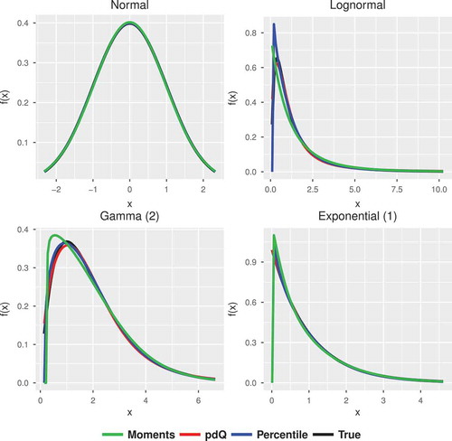
In Table 2 we compare our pdQ method with the moments and percentile matching methods. The pdQ method typically outperforms the existing methods, returning excellent approximations for all of the distributions considered, especially for those that are highly skewed. This is apparent in Figure 1 where the approximated density curves from the pdQ method mimics the true density extremely well compared to the other methods for the lognormal, Gamma and exponential distributions. All methods do very well at approximating the normal density. The non-existence of the first four moments for the selected parameter choice for the Cauchy, Frechet and Dagum distributions makes the moment method inapplicable for those instances. However, both the percentile and the pdQ methods could be used for these distributions.

Table 2. Hellinger distances comparing the performance of the moments, percentile matching and pdQ with quartile matching methods

Distribution	Moments	Percentile	pdQ
Uniform (2,5)	0.0000	0.0000	0.0000^a
Normal (0,1)	0.0000	0.0001	0.0001^a
Lognormal (0,1)	0.0166	0.0189	0.0066^b
Exponential (1)	0.0137	0.0074	0.0000^c
${\chi }_5^2$	0.0098	0.0046	0.0016^a
Pareto (7)	0.0067	0.0077	0.0000^c
Gamma (2)	0.0157	0.0062	0.0019^a
Beta (2,3)	0.0004	0.0007	0.0004^a
Weibull (2)	0.0000	0.0001	0.0000^b
Cauchy (0,1)	NA	0.0002	0.0003^a
Frechet (0,1,1)	NA	0.0215	0.0116^b
Dagum (1,2,3)	NA	0.0099	0.0028^a
Singh-Maddala (1,2,3)	0.0018	0.0007	0.0001^a

^aNo weighting ^bleft weighting ^cright weighting.

Figure 1. Plots of the true and approximating GLD probability densities for several distributions using the moment matching (green), percentile matching (blue) and pdQ (red) methods. The true probability density is the black curve.

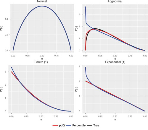
We further investigated the pdQ method and the percentile method by considering the scale—and location-free pdQ plots given in Figure 2. The pdQ curves produced by the pdQ method shows a better approximation to the true pdQ curve compared to those generated by the percentile matching method.

Figure 2. Plots of the pdQ for several distributions using the percentile matching (blue) and pdQ (red) methods. The true pdQ is the black curve.

In Table 3 we provide the chosen parameters of the GLD distribution by the pdQ method. A large value of ${\lambda }_3$ for the exponential is due to the fact that the theoretically optimal value is $\mathrm{\infty }$ (see Section 2.4.2). The pdQ method also chooses the correct optimal choices for the uniform distribution that we considered earlier in Section 2.4.1.

Table 3. Parameters chosen for the generalized lambda distribution using the pdQ method and quartile matching

Distribution	l1	l2	l3	l4	Weight
Uniform (2,5)	3.5	0.6667	1	1	None
Normal (0,1)	0	1.4420	0.1469	0.1469	None
Lognormal (0,1)	0.8038	1.8141	0.7589	−0.7082	Left
Exponential (1)	0	1	30209	0	Right
${\chi }_5^2$	4.0559	0.4977	0.5167	−0.1470	None
Pareto (7)	1	7	19695	−0.1429	Right
Gamma (2)	1.5291	1.1391	0.5840	−0.1867	None
Beta (2,3)	0.3770	5.3836	0.4958	0.2637	None
Weibull (2)	0.8056	2.7931	0.4393	0.0862	Left
Cauchy (0,1)	0	2.3025	-0.8418	-0.8418	None
Frechet (0,1,1)	1.0644	1.7144	0.7167	−1.4507	Left
Dagum (1,2,3)	1.7568	1.5779	0.4593	−0.7716	None
Singh-Maddala (1,2,3)	0.4782	4.4903	0.4647	−0.1661	None

We have also made a Shiny (Chang, Cheng, Allaire, Xie, & McPherson, 2017) application that can be used to find parameters of the GLD for several distributions. The app can be found at https://lukeprendergast.shinyapps.io/GLDlambdas/

We are happy to include other distributions on request and improvements to this application will continue to be made.

5. Extensions

As an another possibility, we consider the Generalized Beta Distribution (GB) with the parameterization below as expressed in the R bda package (Wang, 2015). This parameterization form includes a location parameter ($a$), a scale parameter ($b$) and two shape parameters $\alpha$ and $\beta$. The quantile function is

(5) $Q(u)=a+(b-a)S(u;\alpha ,\beta )$(5)

where $S(u;\alpha ,\beta )$ is the quantile function of the usual beta distribution, also commonly known as the inverse regularized beta function. A closed-form expression for $S(u;\alpha ,\beta )$ exists only if $\alpha =1$, $\beta =1$ or $\alpha =\beta =1$. Further the density quantile function for the GB can be obtained as follows,

(6) $f_Q(u)=\frac{1}{(b-a)q(u)}.$(6)

where $q(u)$ denotes the quantile density function of the beta distribution. The pdQ for the GB can be obtained similarly using numerical integration as a closed-form solution is not available for $\kappa ={\int }_0^1{f}_Q(u)du$.

Table 4 summarizes the performance of the pdQ approach in choosing optimal parameters for the GB distributions in approximating several distributions. Similar results can be found by Karian and Dudewicz (2016) for parameter choices of the GB using the moments method. Excellent approximations can be obtained for most of the distributions such as the Uniform, Normal, exponential, ${\chi }^2$, gamma, beta and triangular distributions using the pdQ approach. The parameterization in 5 indicates that the location and scale are the lower and upper bounds of support for the GB. Therefore, approximations for those parameters get larger for distributions which have infinite support in an effort to capture enough of the density being approximated. Further, shape parameters also can be very large due to the theoretically optimal value being infinite. As an example, both the pdQ method here and the moments matching method in Karian and Dudewicz (2016) provide similar approximations for the normal distribution. The moments matching method approximates the standard normal with parameter choices −1414.214, 1414.214, 999998.848, 999998.848 while the pdQ approach provides similar choices in Table 4. Moreover, Karian and Dudewicz (2016) report that it is possible to further improve this approximation by letting the two shape parameters get even larger. For the standard beta distribution, the theoretically optimal choices for the four GB distribution are the first and second shape parameter values and a location and scale of zero and one respectively. As can be seen in the table, the pdQ approach correctly identifies these parameters.

Table 4. Parameters chosen for the generalized beta distribution with Hellinger distance using pdQ method with quartile matching to choice the best parameters

Distribution	Location	Scale	Shape 1	Shape 2	Hellinger	Weight
Uniform (2,5)	2	5	1	1	0.0000	None
Normal (0,1)	−81.1991	81.2063	3296.9272	3297.2195	0.0000	None
Lognormal (0,1)	0.0358	35,968,259	1.0784	28,694,641	0.0139	Left
Exponential (1)	0	79,194,935	1	79,194,934	0.0000	None
${\chi }_5^2$	0	4,141,322	2.5	2,070,656	0.0000	None
Pareto (7)	0.9973	115,128.1	0.9354	680,085.2	0.0122	Left
Gamma (2)	0	6,421,984	2	6,421,980	0.0000	None
Beta (2,3)	0	1	2	3	0.0000	None
Weibull (2)	−0.0518	3.3441	2.7716	7.2798	0.0007	None
Cauchy (0,1)	−837.5752	829.6024	158,813.3	157,301.6	0.0749	None
Frechet (0,1,1)	−0.1662	6,466,193	0.8929	2,370,934	0.1090	Left
Dagum (1,2,3)	0.4140	32,616,990	1.5629	26,243,197	0.0184	Both
Singh-Maddala (1,2,3)	−0.0160	339,986.2	2.7880	1,592,214	0.0011	Left
Triangular (0,1,0)	0	1	2	1	0.0000	None

We now further look at two specific cases where an exact solution can be obtained for the GB using the pdQ method.

5.1. The uniform distribution

We revisit Section 2.4.1 for the uniform distribution. As described below, we can use the same process to identify the theoretically optimal parameters for the GB. The pdQ for the uniform can be derived as $f_{Q_1}^{\ast }(u)=1$. When $\alpha =1$ and $\beta =1$, the closed-form expression for the quantile function of the beta distribution is found to be $S(u;\alpha =1,\beta =1)=u$ (Sharma & Chakrabarty, 2017). Hence, for these parameter choices, we have the GB pdQ as $f_Q^{\ast }(u)=1$ and equality between the uniform and GB pdQs. As with the beta distribution, the pdQ approach has identified the optimal parameters.

5.2. The triangular distribution

Similarly, let us also consider the triangular distribution with parameters $a=0$, $b=1$ and $c=0$ giving the quantile function $Q(u)=1-(1-u{)}^{1/2}$. Consequently, we can obtain the density quantile function of the triangular distribution as $f_Q(u)=2(1-u{)}^{1/2}$. Further, using ${\int }_0^1{f}_Q(u)du=4/3$, the pdQ of the triangular distribution can be derived as $f_Q^{\ast }(u)=3(1-u{)}^{1/2}/2$. If we consider $\alpha =1$ and $\beta =2$, a closed form solution for the quantile function of the beta distribution can be obtained as $S(u;\alpha =1,\beta =2)=1-(1-u{)}^{1/2}$ (Sharma & Chakrabarty, 2017) which in turn gives the pdQ of the GB distribution as $f_Q^{\ast }(u)=3(1-u{)}^{1/2}/2$. Therefore, we can obtain equality between the triangular and GB pdQs for this parameter choice. Again, the pdQ approach has found the optimal parameters.

6. Discussion

By concentrating on first identifying suitable shape parameters using the probability density quantile function, we have introduced a method for choosing optimal GLD parameters to approximate other distributions. Our method typically outperforms the approaches based on moment and percentile matching, and it is simple and efficient to implement. We also showed that the approach is also suitable for other distributions such as the generalized beta distribution. We are currently investigating estimation methods using some of the ideas developed here in the population setting.

Acknowledgements

The authors would like to thank the two anonymous referees for their thoughtful suggestions and the Editor for their support in providing a revised version.

Disclosure statement

No potential conflict of interest was reported by the authors.

Additional information

Funding

The authors received no direct funding for this research.

Notes on contributors

Dilanka S. Dedduwakumara

Mr. Dilanka S. Dedduwakumara is a PhD candidate and a Statistician in the Department of Mathematics, La Trobe University, Australia. He has a Bachelor of Science (B.Sc.) in Statistics from the University of Colombo, Sri Lanka. He is researching in the fields of quantile-based methods in regards to limited summary information and parameter estimation of Generalized Distributions.

References

- Chang, W., Cheng, J., Allaire, J. J., Xie, Y., & McPherson, J. (2017). shiny: Web Application Framework for R, r package version 1.0.5.
- R Core Team. (2017). R: A language and environment for statistical computing. Vienna, Austria: R Foundation for Statistical Computing.
- Freimer, M., Kollia, G., Mudholkar, G. S., & Lin, C. T. (1988). A study of the generalized Tukey lambda family. Communications in Statistics-Theory and Methods, 17, 3547–11. doi:10.1080/03610928808829820
- Gilchrist, W. (2000). Statistical modelling with quantile functions. Florida: CRC Press.
- Hellinger, E. (1909). Neue begründung der theorie quadratischer formen von unendlichvielen veränderlichen. Journal für die reine und angewandte Mathematik, 136, 210–271.
- Karian, Z., & Dudewicz, E. (1999). Fitting the generalized lambda distribution to data: A method based on percentiles. Communications in Statistics-Simulation and Computation, 28(3), 793–819. doi:10.1080/03610919908813579
- Karian, Z. A., & Dudewicz, E. J. (2003). Comparison of GLD fitting methods: Superiority of percentile fits to moments in L2 norm.
- Karian, Z. A., & Dudewicz, E. J. (2016). Handbook of fitting statistical distributions with R. New York, NY: Chapman and Hall/CRC.
- Lakhany, A., & Mausser, H. (2000). Estimating the parameters of the generalized lambda distribution. Algo Research Quarterly, 3(3), 47–58.
- Parzen, E. (1979). Nonparametric statistical data modeling. Journal of the American Statistical Association, 74, 105–121. doi:10.1080/01621459.1979.10481621
- Pfaff, B. (2016). Financial risk modelling and portfolio optimization with R. UK: John Wiley & Sons.
- Ramberg, J. S., & Schmeiser, B. W. (1974). An approximate method for generating asymmetric random variables. Communications of the ACM, 17(2), 78–82. doi:10.1145/360827.360840
- Sharma, D., & Chakrabarty, T. K. (2017). Some general results on quantile functions for the generalized beta family. Statistics, Optimization & Information Computing, 5(4), 360–377. doi:10.19139/soic.v5i4.312
- Staudte, R. G. (2017). The shapes of things to come: Probability density quantiles. Statistics, 51, 782–800. doi:10.1080/02331888.2016.1277225
- Staudte, R. G., & Sheather, S. J. (1990). Robust estimation and testing (Vol. 918). New York, NY: John Wiley & Sons.
- Staudte, R. G., & Xia, A. (2018). Divergence from, and convergence to, uniformity of probability density quantiles. Entropy, 20(5). doi:10.3390/e20050317
- Tarsitano, A. (2005). Estimation of the generalized lambda distribution parameters for grouped data. Communications in Statistics—Theory and Methods, 34(8), 1689–1709. doi:10.1081/STA-200066334
- Tukey, J. W. (1965). Which part of the sample contains the information? Proceedings of the National Academy of Sciences, 53, 127–134.
- Venables, W. N., & Ripley, B. D. (2002). Modern applied statistics with S (4th ed.). New York: Springer. ISBN 0-387-95457-0.
- Wang, B. (2015). bda: Density Estimation for Grouped Data, R package version 5.1.6.. doi:10.1094/PDIS-09-14-0954-PDN