A hybrid direction algorithm for solving optimal control problems

Abstract

In this paper, we present an algorithm for finding an approximate numerical solution for linear optimal control problems. This algorithm is based on the hybrid direction algorithm developed by Bibi and Bentobache [A hybrid direction algorithm for solving linear programs, International Journal of Computer Mathematics, vol. 92, no.1, pp. 201–216, 2015]. We define an optimality estimate and give a necessary and sufficient condition to characterize the optimality of a certain admissible control of the discretized problem, then we give a numerical example to illustrate the proposed approach. Finally, we present some numerical results which show the convergence of the proposed algorithm to the optimal solution of the presented continuous optimal control problem.

Keywords:

• Optimal control
• linear programming
• hybrid direction algorithm
• optimality estimate
• numerical results

PUBLIC INTEREST STATEMENT

The optimal control theory consists in finding a control which optimizes a functional on a domain described by a system of differential equations, with box and terminal constraints on the control. This theory is applied in various fields of the engineering sciences: aeronautics, physics, finance, etc. For example, finding the minimal time necessary for moving a missile from one starting point to a destination point can be modeled as an optimal control problem, where the constraints are given by the motion equations of the missile. In this work, we have proposed a method which finds a numerical solution for the linear optimal control problem. Our method can be used for the simulation of optimal trajectories of control problems which arise in military applications, finance, etc.

1. Introduction

The optimal control theory consists in finding a control which optimizes a functional on a domain described by a system of differential equations, with box and terminal constraints on the control. This theory is applied in various fields of the engineering sciences: aeronautics, physics, finance, etc. Because of the importance of this theory, several researchers have been interested in the development of effective numerical methods for solving this type of problems. In (Gabasov & Kirillova, 1980; Gabasov, Kirillova, & Prischepova, 1995), the authors developed the adaptive method for solving linear optimal control problems. This method is then generalized for solving general quadratic optimization problems (Bibi, 1994, 1996; Brahmi & Bibi, 2010; Khimoum & Bibi, 2019; Kostina & Kostyukova, 2001).

In (Bentobache, 2013; Bentobache & Bibi, 2016; Bibi & Bentobache, 2011, 2015), the authors proposed a new improvement direction for the adaptive method in order to solve linear programming problems with bounded variables. This direction is called hybrid direction because some of its components take extreme values and the other components take the values of the opposite gradient.

In this paper, we present an algorithm based on this hybrid direction for solving linear optimal control problems. In a similar way to (Bibi & Bentobache, 2015), we define an optimality estimate and give a necessary and sufficient condition to characterize the optimality of a certain admissible control of the discretized problem. Then, we describe a numerical algorithm for finding an approximate solution and we present some numerical results in order to show its convergence.

The paper is organized as follows: In Section 2, we present the problem and give some definitions. In Section 3, we present the details of the proposed algorithm and we give a numerical example to illustrate our approach in Section 4. Finally, we conclude this paper and give some perspectives.

2. Optimal control problem

2.1. State of the problem and definitions

Consider the following terminal optimal control problem:

(1) $\left\{\begin{array}{cccc}J(u)=c^{\prime }x(t^{\ast })\to \underset{u}{max},& (1.1)& \hspace{0.17em}& \hspace{0.17em}\\ \frac{dx}{dt}=\dot{x}(t)=Ax(t)+bu(t),x(t_{\ast })=x_0,& (1.2)& \hspace{0.17em}& \hspace{0.17em}\\ Hx(t^{\ast })=g,& (1.3)& \hspace{0.17em}& \hspace{0.17em}\\ f_{\ast }\le u(t)\le f^{\ast },t\in T=[t_{\ast },t^{\ast }],& (1.4)& \hspace{0.17em}& \hspace{0.17em}\end{array}\right.$(1)

where $J(u)$ is the quality criterion, $A\in {\mathcal{M}}_{n\times n}\left(\mathbb{R}\right)$ is the dynamic matrix of the system, $x(t)\in {\mathbb{R}}^n$ is the state vector of the system, $b\in {\mathbb{R}}^n$, $H\in {\mathcal{M}}_{m\times n}\left(\mathbb{R}\right)$ is a matrix of rank $m\le n$, $g\in {\mathbb{R}}^m$, $u(t)\in \mathbb{R}$ is a piecewise constant control bounded by $f_{\ast },f^{\ast }\in \mathbb{R}$ and $c\in {\mathbb{R}}^n$. The symbol (’) designates the transposition operation.

Definition 1 Any control $u=(u(t),t\in T)$ satisfying the constraints:

$f_{\ast }\le u(t)\le f^{\ast },t\in T=[t_{\ast },t^{\ast }],Hx(t^{\ast })=g,$

is called an admissible control of the problem $(1)$.

An admissible control $u^0=(u^0(t),t\in T)$ is said to be optimal if

$J(u^0)=\underset{u}{max}J(u).$

An admissible control $u^{\epsilon }$ is said to be $\epsilon -$ optimal or suboptimal if

$J(u^0)-J(u^{\epsilon })\le \epsilon ,$

where $\epsilon \ge 0$ is an accuracy chosen in advance.

The solution of the problem consists in the determination of an admissible control $u^0$ which, with the trajectory $x^0$, maximizes the quality criterion $J(u)$:

$J(u^0)=\underset{u}{max}J(u)=\underset{u}{max}{c}^{\prime }x(t^{\ast })=c^{\prime }{x}^0(t^{\ast }).$

The solution of the system $(1.2)$ is given by

(2) $x(t)=F(t)\left(x_0+\underset{t_{\ast }}{\overset{t}{\int }}{F}^{-1}(\tau )bu(\tau )d\tau \right),t\in T,$(2)

where $F(t),t\in T,$ is the solution of the system

$\left\{\begin{array}{cc}\dot{F}(t)=AF(t),& \hspace{0.17em}\\ F(t_{\ast })=I_n,t\in T,& \end{array}\right.$

and the matrix $I_n$ represents the identity matrix of order $n$.

By replacing the expression (2) in the system $(1.1)-(1.3)$, we find

$J(u)=c^{\prime }x(t^{\ast })=c^{\prime }F(t^{\ast })x_0+\underset{t_{\ast }}{\overset{t^{\ast }}{\int }}{c}^{\prime }F(t^{\ast })F^{-1}(t)bu(t)dt,$

$HF(t^{\ast })x_0+\underset{t_{\ast }}{\overset{t^{\ast }}{\int }}HF(t^{\ast })F^{-1}(t)bu(t)dt=g.$

If we set

$c(t)=c^{\prime }F(t^{\ast })F^{-1}(t)b,$

$\varphi (t)=HF(t^{\ast })F^{-1}(t)b,$

$g_0=g-HF(t^{\ast })x_0,$

then we get the following equivalent problem:

(3) $\left\{\begin{array}{cccc}J(u)=c^{\prime }F(t^{\ast })x_0+\underset{t_{\ast }}{\overset{t^{\ast }}{\int }}c(t)u(t)dt\to \underset{u}{max},& (3.1)& \hspace{0.17em}& \hspace{0.17em}\\ \underset{t_{\ast }}{\overset{t^{\ast }}{\int }}\varphi (t)u(t)dt=g_0,& (3.2)& \hspace{0.17em}& \hspace{0.17em}\\ f_{\ast }\le u(t)\le f^{\ast },t\in T=[t_{\ast },t^{\ast }].& (3.3)& \hspace{0.17em}& \hspace{0.17em}\end{array}\right.$(3)

2.2. Discretization of the initial problem

We choose a subset $T_h=\{t_{\ast },t_{\ast }+h,\dots ,t^{\ast }-h\},$ where $h=\frac{t^{\ast }-t_{\ast }}{N}$ and $N\in {\mathbb{N}}^{\ast }.$ Let the function $u(t),t\in T$, be a piecewise constant control such that

$u(t)\equiv u(\tau ),t\in [\tau ,\tau +h[,\tau \in T_h.$

Using this discretization, the problem $(3.1)-(3.3)$ becomes:

(4) $\left\{\begin{array}{cccc}J(u)=c^{\prime }F(t^{\ast })x_0+\sum _{\tau \in T_h}q(\tau )u(\tau )\to \underset{u}{max},& (4.1)& \hspace{0.17em}& \hspace{0.17em}\\ \sum _{\tau \in T_h}d(\tau )u(\tau )=g_0,& (4.2)& \hspace{0.17em}& \hspace{0.17em}\\ f_{\ast }\le u(\tau )\le f^{\ast },\tau \in T_h,& (4.3)& \hspace{0.17em}& \hspace{0.17em}\end{array}\right.$(4)

where

(5) $q(\tau )=\underset{\tau }{\overset{\tau +h}{\int }}c(s)ds\mathrm{a}\mathrm{n}\mathrm{d}d(\tau )=\underset{\tau }{\overset{\tau +h}{\int }}\varphi (s)ds.$(5)

2.3. Support control

The set $T_B=\{{\tau }_i,i=\overline{1,m}\}\subset T_h,$ is called a support if the corresponding matrix $P_B=(d(\tau ),\tau \in T_B)\in {\mathcal{M}}_{m\times m}(\mathbb{R})$ is nonsingular.

The pair $\{u,T_B\}$ formed by the admissible control $u$ and the support $T_B$ is called a support control of the problem $(4)$. The latter is said to be nondegenerate if $f_{\ast }<u(\tau )<f^{\ast },\tau \in T_B.$

2.4. Increment formula of the functional

Let $\{u,T_B\}$ be a support control and $x(t),t\in T,$ its corresponding trajectory. Using the support $T_B$, we construct the vector of the potentials $\nu \in {\mathbb{R}}^m$ and the cocontrol vector $E(\tau ),\tau \in T_h$, as follows:

(6) ${\nu }^{\prime }=q_B^{\prime }{P}_B^{-1},E(\tau )={\nu }^{\prime }d(\tau )-q(\tau ),$(6)

where $q_B=(q(\tau ),\tau \in T_B)$, $E_B=(E(\tau ),\tau \in T_B)=0$.

Consider another control

$\bar{u}(t)=u(t)+\mathrm{\Delta }u(t),t\in T,$

and the corresponding trajectory

$\bar{x}(t)=x(t)+\mathrm{\Delta }x(t),t\in T.$

Then, the increment of the functional $(4.1)$ is given by

$\mathrm{\Delta }J(u)=J(\bar{u})-J(u)=-\sum _{\tau \in T_N}E(\tau )\mathrm{\Delta }u(\tau ),T_N=T_h\mathrm{\setminus }{T}_B.$

The following theorem gives a necessary and sufficient condition of optimality for an admissible control $u$ of the problem $(4)$.

Theorem 1 (Gabasov et al., 1995) The following relationships:

$\left\{\begin{array}{cc}u(\tau )=f_{\ast },& ifE(\tau )>0,\\ u(\tau )=f^{\ast },& ifE(\tau )<0,\\ f_{\ast }\le u(\tau )\le f^{\ast },& ifE(\tau )=0,\tau \in T_N,\end{array}\right.$

are sufficient, and in the case of the nondegeneracy of the support control $\{u,T_B\}$ also necessary, for the optimality of the admissible control $u.$

3. An iteration of the hybrid direction algorithm

Let $\{u,T_B\}$ be a support control for the problem $(4)$ and $\eta \in [0,1]$. Define the following sets:

$T_N^{+}=\{\tau \in T_N:E(\tau )>\eta \left(u(\tau )-f_{\ast }\right)\},$

$T_N^{-}=\{\tau \in T_N:E(\tau )<\eta \left(u(\tau )-f^{\ast }\right)\},$

$T_N^{P^{+}}=\{\tau \in T_N:0<E(\tau )\le \eta \left(u(\tau )-f_{\ast }\right)\},$

$T_N^{P^{-}}=\{\tau \in T_N:\eta \left(u(\tau )-f^{\ast }\right)\le E(\tau )<0\},$

$T_N^{P^0}=\{\tau \in T_N:E(\tau )=0\},$

$T_N^P=\{\tau \in T_N:\eta \left(u(\tau )-f^{\ast }\right)\le E(\tau )\le \eta \left(u(\tau )-f_{\ast }\right)\}=T_N^{P^{+}}\cup T_N^{P^{-}}\cup T_N^{P^0}.$

Then

$T_h=T_N^{+}\cup T_N^{-}\cup T_N^P\cup T_B.$

Recall that the suboptimality estimate $\beta (u,T_B)$ is given by the following formula (Gabasov et al., 1995):

$\beta (u,T_B)=\sum _{\tau \in T^{+}}E(\tau )(u(\tau )-f_{\ast })+\sum _{\tau \in T^{-}}E(\tau )(u(\tau )-f^{\ast }),$

where $T^{+}=T_N^{+}\cup T_N^{P^{+}}$ and $T^{-}=T_N^{-}\cup T_N^{P^{-}}.$

We call optimality estimate, the quantity $\gamma (\eta ,u,T_B)$ defined by:

(7) $\left\{\begin{array}{cc}\sum _{\tau \in T_N^{+}}E(\tau )(u(\tau )-f_{\ast })+\sum _{\tau \in T_N^{-}}E(\tau )(u(\tau )-f^{\ast })+\frac{1}{\eta }\sum _{\tau \in T_N^{P^{+}}\cup T_N^{P^{-}}}{E}^2(\tau ),& \mathrm{i}\mathrm{f}\eta >0,\\ \beta (u,T_B),& \mathrm{i}\mathrm{f}\eta =0.\end{array}\right.$(7)

Theorem 2 (Necessary and sufficient condition of optimality (Bibi & Bentobache, 2015))

Let $\{u,T_B\}$ be a support control for the problem $(4)$ and $\eta >0$. Then the condition $\gamma (\eta ,u,T_B)=0$ is sufficient and, in the case of the nondegeneracy of the support control $\{u,T_B\}$ also necessary, for the optimality of the admissible control $u$.

Let $\{u,T_B\}$ be a starting support control of the problem $(4)$, for which the optimality criterion is not satisfied. An iteration of the hybrid direction algorithm consists in moving from $\{u,T_B\}$ to $\{\bar{u},{\bar{T}}_B\}$, where $\bar{u}=u+{\theta }^0\mathrm{\Delta }u.$ This passage is done in two steps:

1. Change of control: $u\to \bar{u}.$

2. Change of support: $T_B\to {\bar{T}}_B.$

3.1. Change of control

Let $\{u,T_B\}$ be a support control for the problem $(4)$ and $\eta \in [0,1]$. We compute $\gamma (\eta ,u,T_B)$ with the formula (7). If $\gamma (\eta ,u,T_B)=0,$ then the support control $\{u,T_B\}$ is optimal, otherwise we define the admissible improvement direction $\mathrm{\Delta }u(\tau )$ as follows:

(8) $\mathrm{\Delta }u(\tau )=\left\{\begin{array}{cc}{f}_{\ast }-u(\tau ),& \mathrm{f}\mathrm{o}\mathrm{r}\tau \in T_N^{+},\\ f^{\ast }-u(\tau ),& \mathrm{f}\mathrm{o}\mathrm{r}\tau \in T_N^{-},\\ \frac{-E(\tau )}{\eta },& \mathrm{f}\mathrm{o}\mathrm{r}\tau \in T_N^P,\eta \ne 0,\\ 0,& \mathrm{f}\mathrm{o}\mathrm{r}\tau \in T_N^P,\eta =0,\\ \mathrm{\Delta }u(\tau ),& \mathrm{f}\mathrm{o}\mathrm{r}\tau \in T_B,\end{array}\right.$(8)

where $\mathrm{\Delta }{u}_B=-P_B^{-1}{P}_N\mathrm{\Delta }{u}_N,$ $P_N=(d(\tau ),\tau \in T_N)$ and $\mathrm{\Delta }{u}_N=(\mathrm{\Delta }u(\tau ),\tau \in T_N).$ This direction is called a hybrid direction (Bibi & Bentobache, 2015). The direction $\mathrm{\Delta }u(\tau )$ is an admissible one for the problem $(4)$. Indeed,

$\sum _{\tau \in T_h}d(\tau )\bar{u}(\tau )=\sum _{\tau \in T_h}d(\tau )u(\tau )+{\theta }^0\sum _{\tau \in T_h}d(\tau )\mathrm{\Delta }u(\tau )$

$=\sum _{\tau \in T_h}d(\tau )u(\tau )+{\theta }^0(P_N\mathrm{\Delta }{u}_N+P_B\mathrm{\Delta }{u}_B)$

$=\sum _{\tau \in T_h}d(\tau )u(\tau )+{\theta }^0(P_N\mathrm{\Delta }{u}_N-P_B{P}_B^{-1}{P}_N\mathrm{\Delta }{u}_N)$

$=\sum _{\tau \in T_h}d(\tau )u(\tau )$

$=g_0.$

To improve the objective function while remaining within the admissible domain, we compute the step ${\theta }^0$ along the direction $\mathrm{\Delta }u(\tau )$:

(9) ${\theta }^0=min\{\theta ({\tau }_1),1\},$(9)

where $\theta ({\tau }_1)=min\{\theta (\tau ),\tau \in T_B\},$

with

(10) $\theta (\tau )=\left\{\begin{array}{cc}\frac{f^{\ast }-u(\tau )}{\mathrm{\Delta }u(\tau )},& if\mathrm{\Delta }u(\tau )>0,\\ \\ \frac{f_{\ast }-u(\tau )}{\mathrm{\Delta }u(\tau )},& if\mathrm{\Delta }u(\tau )<0,\\ \\ \mathrm{\infty },& if\mathrm{\Delta }u(\tau )=0.\end{array}\right.$(10)

Then, the new admissible control will be:

(11) $\bar{u}(\tau )=u(\tau )+{\theta }^0\mathrm{\Delta }u(\tau ),$(11)

where $\mathrm{\Delta }u(\tau )$ and ${\theta }^0$ are defined by relationships (8) and (9) respectively.

The increment of the objective function is then

$\mathrm{\Delta }J(u)=-{\theta }^0\sum _{\tau \in T_N}E(\tau )\mathrm{\Delta }u(\tau )$

$=-{\theta }^0\sum _{\tau \in T_N^{+}}E(\tau )\mathrm{\Delta }u(\tau )-{\theta }^0\sum _{\tau \in T_N^{-}}E(\tau )\mathrm{\Delta }u(\tau )-{\theta }^0\sum _{\tau \in T_N^{p^{+}}\cup T_N^{P^{-}}}E(\tau )\mathrm{\Delta }u(\tau )$

$={\theta }^0\sum _{\tau \in T_N^{+}}E(\tau )(u(\tau )-f_{\ast })+{\theta }^0\sum _{\tau \in T_N^{-}}E(\tau )(u(\tau )-f^{\ast })+{\theta }^0\sum _{\tau \in T_N^{p^{+}}\cup T_N^{p^{-}}}\frac{E^2(\tau )}{\eta }$

$={\theta }^0\gamma (\eta ,u,T_B)\ge 0.$

So $J(\bar{u})>J(u)$, for ${\theta }^0>0$.

Corollary 1 (Bibi & Bentobache, 2015)

If ${\theta }^0=1$ and $T_N^{P^{+}}\cup T_N^{P^{-}}=\mathrm{\varnothing },$ then $\bar{u}$ is optimal.

3.2. Change of support

If for the support control $\{\bar{u},T_B\}$ of the problem $(4)$, we have ${\theta }^0<1,$ then we change $T_B$ by ${\bar{T}}_B$ using the dual method. For this, we compute the vector $\omega$ and the number ${\alpha }_0$ as follows:

$\omega (\tau )=u(\tau )+\mathrm{\Delta }u(\tau ),\tau \in T_h\mathrm{a}\mathrm{n}\mathrm{d}{\alpha }_0=\omega ({\tau }_1)-\bar{u}({\tau }_1).$

Then, the new cocontrol will be given by:

$\bar{E}(\tau )=E(\tau )+{\sigma }^0\delta (\tau ),\tau \in T_h,$

where $\delta (\tau )$ is the dual direction and ${\sigma }^0$ the dual step, which are computed as follows:

(12) $\delta (\tau )=\left\{\begin{array}{cc}0,& \mathrm{i}\mathrm{f}\tau \in T_B\mathrm{\setminus }\{{\tau }_1\},\\ -1,& \mathrm{i}\mathrm{f}{\alpha }_0>0,\tau ={\tau }_1,\\ +1,& \mathrm{i}\mathrm{f}{\alpha }_0<0,\tau ={\tau }_1,\\ {{\delta }^{\prime }}_B{P}_B^{-1}d(\tau ),& \mathrm{f}\mathrm{o}\mathrm{r}\tau \in T_N,{{\delta }^{\prime }}_B=(\delta (\tau ),\tau \in T_B),\end{array}\right.$(12)

(13) ${\sigma }^0=\sigma ({\tau }_0)=\underset{\tau \in T_N}{min}\sigma (\tau ),$(13)

where

$\sigma (\tau )=\left\{\begin{array}{cc}\frac{-E(\tau )}{\delta (\tau )},& \mathrm{i}\mathrm{f}E(\tau )\delta (\tau )<0,\\ 0,& \mathrm{i}\mathrm{f}E(\tau )=0,\delta (\tau )<0,\omega (\tau )\ne f^{\ast },\\ 0,& \mathrm{i}\mathrm{f}E(\tau )=0,\delta (\tau )>0,\omega (\tau )\ne f_{\ast },\\ +\mathrm{\infty },& \mathrm{e}\mathrm{l}\mathrm{s}\mathrm{e}\mathrm{w}\mathrm{h}\mathrm{e}\mathrm{r}\mathrm{e},\tau \in T_N.\end{array}\right.$

The following new support is then obtained:

${\bar{T}}_B=(T_B\mathrm{\setminus }\{{\tau }_1\})\cup \{{\tau }_0\}.$

3.3. Scheme of the hybrid direction algorithm

Let $\{u,T_B\}$ be a support control for the problem $(4)$ and $\eta$ a real number such that $\eta \in [0,1]$. In order to take into account the specificity of the studied linear optimal control problem, we present in this section a slightly modified version of the algorithm presented in (Bibi & Bentobache, 2015). Indeed, if ${\theta }^0=1$ and $T_N^{P^{+}}\cup T_N^{P^{-}}\ne \mathrm{\varnothing }$, then we reduce the value of the parameter $\eta$ by setting $\eta =\eta /2$ and we start a new iteration with the new control $\bar{u}$. The scheme of the hybrid direction algorithm for solving the linear optimal control problem is described in the following steps:

Algorithm 1

(1) Compute $d(\tau ),q(\tau ),\nu ,E(\tau )$ with relationships (5)-(6);

(2) Determine the sets $T_N^{+}$, $T_N^{-}$, $T_N^{P^{+}}$ and $T_N^{P^{-}}$;

(3) Compute $\gamma (\eta ,u,T_B)$ with the formula (7);

(4) If $\gamma (\eta ,u,T_B)=0$, then the algorithm stops with $\{u,T_B\}$, an optimal support control for the discretized problem;

(5) Compute the improvement direction $\mathrm{\Delta }u(\tau )$ using the relationship (8);

(6) Compute $\theta ({\tau }_1)=\underset{\tau \in T_B}{min}\theta (\tau ),$ where $\theta (\tau )$ is determined by (10);

(7) Compute ${\theta }^0=min\{1,\theta ({\tau }_1)\},$ $\bar{u}(\tau )=u(\tau )+{\theta }^0\mathrm{\Delta }u(\tau ),\tau \in T_h,$ and

$J(\bar{u})=J(u)+{\theta }^0\gamma (\eta ,u,T_B);$

(8) If ${\theta }^0=1$, then

(8.1)—If $T_N^{P^{+}}\cup T_N^{P^{-}}=\mathrm{\varnothing }$, then $\bar{u}(\tau )$ is optimal. Stop.

(8.2)—Else, set $\eta =\eta /2$, $u(\tau )=\bar{u}(\tau )$, $J(u)=J(\bar{u})$ and go to step (2).

(9) Compute the dual direction $\delta (\tau ),\tau \in T_h,$ using the relationship (12);

(10) Compute the dual step ${\sigma }^0$ and determine ${\tau }_0$ using the relationship (13);

(11) Set $\bar{E}(\tau )=E(\tau )+{\sigma }^0\delta (\tau ),\tau \in T_h,$ ${\bar{T}}_B=(T_B\mathrm{\setminus }\{{\tau }_1\})\cup \{{\tau }_0\}$;

(12) Set $u(\tau )=\bar{u}(\tau )$, $T_B={\bar{T}}_B$, $J(u)=J(\bar{u})$, $E(\tau )=\bar{E}(\tau )$ and go to step (2).

4. Numerical example

Consider the following problem

(14) $\left\{\begin{array}{cc}J(u)=c^{\prime }x(2)\to \underset{u}{max},& \hspace{0.17em}\\ \dot{x}(t)=Ax(t)+bu(t),x(0)=0,& \hspace{0.17em}\\ Hx(2)=g,& \hspace{0.17em}\\ -1\le u(t)\le 1,t\in T=[0,2],& \hspace{0.17em}\end{array}\right.$(14)

with

$A=\left(\begin{array}{cc}0& 1\\ 0& 0\\ \hspace{0.17em}& \hspace{0.17em}\end{array}\right),b=\left(\begin{array}{c}0\\ 1\\ \hspace{0.17em}\end{array}\right),H=(1,-2),g=\frac{1}{2},c=\left(\begin{array}{c}0\\ 1\\ \hspace{0.17em}\end{array}\right).$

We have

$F(t)=\left(\begin{array}{cc}1& t\\ 0& 1\\ \hspace{0.17em}& \hspace{0.17em}\end{array}\right),F^{-1}(t)=\left(\begin{array}{cc}1& -t\\ 0& 1\\ \hspace{0.17em}& \hspace{0.17em}\end{array}\right),$

$c(t)=c^{\prime }F(2)F^{-1}(t)b=1,\varphi (t)=HF(2)F^{-1}(t)b=-t.$

Consider the admissible control

$u(t)=\left\{\begin{array}{cc}\frac{1}{2},& \mathrm{i}\mathrm{f}t\in [0,1[\\ -\frac{1}{2},& \mathrm{i}\mathrm{f}t\in [1,2].\end{array}\right.$

The corresponding trajectory is

$x(t)=\left(\begin{array}{c}\frac{t^2}{4}\\ \frac{t}{2}\\ \hspace{0.17em}\end{array}\right),\mathrm{i}\mathrm{f}t\in [0,1[$

and

$x(t)=\left(\begin{array}{c}\frac{-t^2}{4}+t-\frac{1}{2}\\ \frac{-t}{2}+1\\ \hspace{0.17em}\end{array}\right),\mathrm{i}\mathrm{f}t\in [1,2].$

We choose $h=0.5$ and $\eta =1.$ We take the support control $\{u,T_B\}$ for the problem (14), with $T_B=\{1\}$.

Iteration 1.

$P_B=\underset{1}{\overset{\frac{3}{2}}{\int }}-sds=-\frac{5}{8},P_B^{-1}=-\frac{8}{5},q_B=\underset{1}{\overset{\frac{3}{2}}{\int }}ds=\frac{1}{2},$

${\nu }^{\prime }=\frac{1}{2}\times \frac{-8}{5}=-\frac{4}{5},E(\tau )=\frac{2}{5}(\tau -1),$

$T_N=\left\{0,\frac{1}{2},\frac{3}{2}\right\},$

$T_N^{+}=\{\tau \in T_N:\frac{2}{5}(\tau -1)>\left(u(\tau )+1\right)\}=\mathrm{\varnothing },$

$T_N^{P^{+}}=\{\tau \in T_N:0<\frac{2}{5}(\tau -1)\le \left(u(\tau )+1\right)\}=\left\{\frac{3}{2}\right\},$

$T_N^{-}=\{\tau \in T_N:\frac{2}{5}(\tau -1)<\left(u(\tau )-1\right)\}=\mathrm{\varnothing },$

$T_N^{P^{-}}=\{\tau \in T_N:\left(u(\tau )-1\right)\le \frac{2}{5}(\tau -1)<0\}=\left\{0,\frac{1}{2}\right\}.$

We compute the optimality estimate:

$\gamma (\eta ,u,T_B)=E^2(0)+E^2\left(\frac{1}{2}\right)+E^2\left(\frac{3}{2}\right)=\frac{6}{25},$

so the control $u$ is not optimal.

Change of control:

We compute $\mathrm{\Delta }u(\tau )$

$\mathrm{\Delta }u(\tau )=\left\{\begin{array}{cc}+\frac{2}{5},& \mathrm{i}\mathrm{f}\tau =0,\\ +\frac{1}{5},& \mathrm{i}\mathrm{f}\tau =\frac{1}{2},\\ +\frac{2}{25},& \mathrm{i}\mathrm{f}\tau =1,\\ -\frac{1}{5},& \mathrm{i}\mathrm{f}\tau =\frac{3}{2}.\end{array}\right.$

The step along the direction $\mathrm{\Delta }u(\tau )$ is computed as follows:

We have $\mathrm{\Delta }u(1)=\frac{2}{25},$ then $\theta ({\tau }_1)=\frac{1-\frac{1}{2}}{\frac{2}{25}}=\frac{75}{4}$ and ${\theta }^0=1.$

Hence, the new control is given by:

$\bar{u}(\tau )=\left\{\begin{array}{cc}+\frac{9}{10},& \mathrm{i}\mathrm{f}\tau =0,\\ +\frac{7}{10},& \mathrm{i}\mathrm{f}\tau =\frac{1}{2},\\ -\frac{21}{50},& if\tau =1,\\ -\frac{7}{10},& \mathrm{i}\mathrm{f}\tau =\frac{3}{2}.\end{array}\right.$

We have ${\theta }^0=1$ and $T_N^{P^{+}}\cup T_N^{P^{-}}\ne \mathrm{\varnothing },$ so we set

$\eta =\eta /2=1/2,E(\tau )=\frac{2}{5}(\tau -1),u(\tau )=\bar{u}(\tau ).$

Iteration 2. For this iteration, we have

$T_N^{+}=\left\{\frac{3}{2}\right\},T_N^{-}=\left\{0,\frac{1}{2}\right\},T_N^P=\mathrm{\varnothing }\mathrm{a}\mathrm{n}\mathrm{d}\gamma (\eta ,u,T_B)=\frac{4}{25}.$

We compute the direction $\mathrm{\Delta }u(\tau )$:

$\mathrm{\Delta }u(\tau )=\left\{\begin{array}{cc}+\frac{1}{10},& \mathrm{i}\mathrm{f}\tau =0,\\ +\frac{3}{10},& \mathrm{i}\mathrm{f}\tau =\frac{1}{2},\\ +\frac{11}{50},& if\tau =1,\\ -\frac{3}{10},& \mathrm{i}\mathrm{f}\tau =\frac{3}{2}.\end{array}\right.$

We have $\mathrm{\Delta }u(1)=\frac{11}{50},$ hence $\theta ({\tau }_1)=\frac{1+\frac{21}{50}}{\frac{11}{50}}=\frac{71}{11}$ and ${\theta }^0=1.$ So

$\bar{u}(\tau )=\left\{\begin{array}{cc}+1,& \mathrm{i}\mathrm{f}\tau =0,\\ +1,& \mathrm{i}\mathrm{f}\tau =\frac{1}{2},\\ -\frac{1}{5},& \mathrm{i}\mathrm{f}\tau =1,\\ -1,& \mathrm{i}\mathrm{f}\tau =\frac{3}{2}.\end{array}\right.$

Since ${\theta }^0=1$ and $T_N^{P^{+}}\cup T_N^{P^{-}}=\mathrm{\varnothing },$ then the control

$u^0(\tau )=\left\{\begin{array}{cc}+1,& \mathrm{i}\mathrm{f}\tau =0,\\ +1,& \mathrm{i}\mathrm{f}\tau =\frac{1}{2},\\ -\frac{1}{5},& \mathrm{i}\mathrm{f}\tau =1,\\ -1,& \mathrm{i}\mathrm{f}\tau =\frac{3}{2},\end{array}\right.$

is optimal for the discretized problem, with $J(u^0)=\frac{2}{5}$. Therefore, the control

$u(t)=\left\{\begin{array}{cc}1,& \mathrm{i}\mathrm{f}t\in [0,1[\\ -\frac{1}{5},& \mathrm{i}\mathrm{f}t\in [1,\frac{3}{2}[\\ -1,& \mathrm{i}\mathrm{f}t\in [\frac{3}{2},2],\end{array}\right.$

is an approximate solution of the original problem (14).

In order to find a good approximate solution for the original continuous problem (14), we have implemented the discretization technique using the Cauchy formula and the hybrid direction algorithm with MTALB2018a. The developed solver was tested on a computer surface pro 2, with 4GO of memory and processor Intel(R) Core(TM) i5-4300U CPU 1.90GHz 2.50GHz, running under Microsoft Window 10 operating system.

The initialization approach proposed in (Bentobache & Bibi, 2012) can be used to compute an initial admissible support control, however we have initialized the hybrid direction algorithm with the following obvious admissible control:

$u(t)=\left\{\begin{array}{cc}\frac{1}{2},& \mathrm{i}\mathrm{f}t\in [0,1[\\ -\frac{1}{2},& \mathrm{i}\mathrm{f}t\in [1,2].\\ \hspace{0.17em}& \hspace{0.17em}\end{array}\right.$

In Table 1, we report numerical results for different values of $N$, where $CP{U}_1$, $CP{U}_2$, $IT$ and $J^0$ represent respectively the cpu time of the discretization phase, the execution time, the number of iterations of the hybrid direction algorithm and the optimal value of the quality criterion of (14). We plot the optimal control in terms of $t$ for $N=5000$ (Figure 1) and we plot the optimal objective values of the linear program (4) corresponding to the problem (14) in terms of $N$ (Figure 2).

Note that for large values of $N$, our method converges to the optimal value of the continuous original problem $J^{\ast }=0.4495$. Furthermore, we can see from Graph of Figure 1, that the commutation time is approximately equal to 1.23 sec.

Figure 1. Graph of the optimal control in terms of $t$ for $N=5,000$.

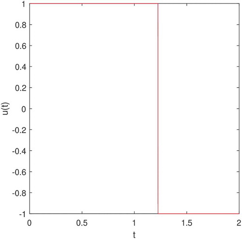
Figure 2. Graph of the objective function value in terms of $N$.

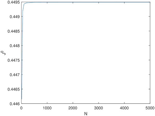
Table 1. Numerical simulation results for the problem (14)

N	$CP{U}_1$	$CP{U}_2$	$IT$	$J^0$
10	0.2689	0.0397	9	0.4,461,538,462
50	1.0252	0.0177	38	0.4,491,803,279
100	1.5805	0.0191	71	0.4,494,308,943
200	3.3212	0.0175	134	0.4,494,693,878
500	7.9160	0.0492	320	0.4,494,877,651
1,000	16.1820	0.1482	628	0.4,494,889,796
2,000	32.6202	0.5174	1243	0.4,494,895,876
3,000	47.3245	1.0210	1856	0.4,494,897,052
5,000	80.9802	3.2498	3082	0.4,494,897,273

5. Conclusion

In this paper, we applied the hybrid direction algorithm developed in (Bibi & Bentobache, 2015) to find an approximate optimal solution to a linear optimal control problem. A numerical example was given to illustrate the described algorithm, and some numerical simulation results were presented in order to show the convergence of our algorithm to the optimal solution of the continuous problem. In a future work, we will compare the presented approach with classical approaches on practical optimal control problems.

Correction

This article has been republished with minor changes. These changes do not impact the academic content of the article.

Acknowledgements

The authors are indebted to Dr. Mohamed Aliane who supplied them the matlab code of the Cauchy discretization technique and to the anonymous referees whose comments and suggestions have improved the quality of this paper.

Additional information

Funding

The authors received no direct funding for this research.

Notes on contributors

Mohamed Abdelaziz Zaitri

Mohamed Abdelaziz Zaitri received a DES degree in Mathematics from the Higher Normal School of Kouba (2011), Algeria, a master degree (2014) from the University of Bejaia. He is a PhD student at the Department of Operational Research, University of Bejaia, Algeria.

Mohand Ouamer Bibi

Mohand Ouamer Bibi received a DES degree in Mathematical Analysis (1980) from the USTHB University, Algeria, a master degree (1982) and PhD (1986) in Applied Mathematics from the University of Minsk, Belarus. He is a Full Professor at the Department of Operational Research and the leader of the research group “Optimization and Optimal Control” at the LaMOS Research Unit, University of Bejaia, Algeria.

Mohand Bentobache

Mohand Bentobache received his engineering degree in operational research (2002), master degree (2005), PhD (2013) and HDR (2015) in Applied Mathematics from the University of Bejaia, Algeria. He is an Associate Professor at the Department of Technology and the leader of the research group “Numerical Analysis and Optimization” at the Laboratory of LMPA, University of Laghouat, Algeria.

References

- Bentobache, M. (2013). On mathematical methods of linear and quadratic programming (PhD thesis), University of Bejaia, Bejaia, Algeria.
- Bentobache, M., & Bibi, M. O. (2012). A two-phase support method for solving linear programs: Numerical experiments. Mathematical Problems in Engineering, 2012. Article ID 482193, doi:10.1155/2012/482193
- Bentobache, M., & Bibi, M. O. (2016). Numerical methods of linear and quadratic programming. Germany (in French): French Academic Editions.
- Bibi, M. O. (1994). Optimization of a linear dynamic system with double terminal constraints on the trajectories. Optimization, 30(4), 359–12. doi:10.1080/02331939408843998
- Bibi, M. O. (1996). Support method for solving a linear-quadratic problem with polyhedral constraints on control. Optimization, 37(2), 139–147. doi:10.1080/02331939608844205
- Bibi, M. O., & Bentobache, M. (2011). The adaptive method with hybrid direction for solving linear programming problems with bounded variables. Proceedings of COSI’2011 pp. 80–91, 24–27 April, Algeria: University of Guelma.
- Bibi, M. O., & Bentobache, M. (2015). A hybrid direction algorithm for solving linear programs. International Journal of Computer Mathematics, 92(1), 201–216. doi:10.1080/00207160.2014.890188
- Brahmi, B., & Bibi, M. O. (2010). Dual support method for solving convex quadratic programs. Optimization, 59(6), 851–872. doi:10.1080/02331930902878341
- Gabasov, R., & Kirillova, F. M. (1980). Methods of linear programming (Vol. 3). Edition of the Minsk University, Minsk (in Russian).
- Gabasov, R., Kirillova, F. M., & Prischepova, S. V. (1995). Optimal feedback control. London: Springer-Verlag.
- Khimoum, N., & Bibi, M. O. (2019). Primal-dual method for solving a linear-quadratic multi-input optimal control problem. Optimization Letters. doi:10.1007/s11590-018-1375-2
- Kostina, E. A., & Kostyukova, O. I. (2001). An algorithm for solving quadratic programming problems with linear equality and inequality constraints. Computational Mathematics and Mathematical Physics, 41(7), 960–973.