Model selection among growth curve models that have the same number of parameters

Abstract

A model selection method was proposed to determine the most appropriate model among growth curve models that have the same number of parameters. It uses a measure of mean relative squared error and regression equations from difference equations for growth curve models. The difference equations have exact solutions that are on exact solutions of differential equations as growth curve models. The regression equations from the difference equations perfectly reproduce their parameter estimates. The proposed method selects an appropriate model when data are on an exact solution of a differential equation. It was verified to be practical with six actual datasets when the Gompertz curve and logistic curve models, which are often used for forecasting, were alternative growth curve models.

Keywords:

• model selection
• Gompertz curve model
• logistic curve model
• difference equation
• exact solution
• applied discrete systems

PUBLIC INTEREST STATEMENTS

Growth curve models such as Gompertz and logistic are often used for forecasting in various fields. Selecting an appropriate model is crucial for forecasting success because forecasting using an inappropriate model can result in seriously incorrect forecasts. However, growth curve models have tended to be selected on an ad hoc basis. In this paper, a model selection method was proposed to determine the most appropriate model among growth curve models that have the same number of parameters. It uses a measure of mean relative squared error and regression equations from difference equations for growth curve models. The difference equations have exact solutions that are on exact solutions of differential equations as growth curve models. The regression equations from the difference equations perfectly reproduce their parameter estimates. The proposed method selects an appropriate model when data are on an exact solution of a differential equation. It was verified to be practical with six actual datasets.

1. Introduction

Growth curve models such as Gompertz and logistic curve models are often used for forecasting in various fields, e.g., market development (Bass, 1969; Bemmaor, 1992; Gregg, Hossel, & Richardson, 1964; Gupta & Jain, 2012; Guseo & Guidolin, 2009; Lechman, 2015; Martino, 2003; Meade, 1984; Satoh, 2001), agriculture (Aggrey, 2002; Knízetová, Hyánek, Kníze, & Roubícek, 1991; Narinc, Karaman, Firat, & Aksoy, 2010; Roush & Branton, 2005), computer worm infections (Satoh & Uchida, 2010), and software reliability engineering (Satoh, 2000; Satoh & Yamada, 2002; Yamada, 2014; Yamada, Inoue, & Satoh, 2002; Yamada & Tamura, 2016).

Accurate parameter estimation is indispensable for accurate forecasting with a growth curve model. Inaccurate parameter estimation provides inaccurate forecasting because estimating parameters of the models is equivalent to forecasting with the models. Accurate parameter estimation is accomplished with difference equations that have exact solutions (Satoh, 2000; Satoh, 2001; Satoh & Yamada, 2002; Yamada et al., 2002). The exact solutions are on exact solutions of differential equations as growth curve models. Thus, the difference equations conserve the properties of the differential Equations Hirota, 1979; Hirota, 2000; Hirota & Takahashi, 2003; Satoh, 2000. We call the difference equations integrable difference equations. The integrable difference equations are easily applied to regression equations to obtain parameter estimates and have advantages over ordinary difference Equations Satoh, 2001. Furthermore, forecasting with the difference equations yields accurate parameter estimates in the early stage (Satoh, 2000; Satoh & Yamada, 2002). Such applications of the integrable difference equations are called “applied discrete systems.”

Accurate parameter estimation alone, however, is not enough to provide accurate forecasting. For accurate forecasting, an appropriate model must be selected and parameters accurately estimated. Selecting an appropriate model is crucial for forecasting success (Martino, 2003) because forecasting using an inappropriate model can result in seriously incorrect forecasts (Chu, Wu, Kao, & Yen, 2009; Martino, 2003; Yamakawa, Rees, Salas, & Alva, 2013). However, growth curve models tend to be selected on an ad hoc basis (Chu et al., 2009; Yamakawa et al., 2013). There are only a few frameworks for model selection, though there have been several empirical studies (e.g., Meade & Islam, 1995).

There are four methods of selecting the more appropriate model from the logistic and Gompertz curve models, which are often used for forecasting in various fields, e.g., market development (Gregg et al., 1964; Gupta & Jain, 2012; Lechman, 2015; Martino, 2003; Meade, 1984), agriculture (Aggrey, 2002; Knízetová et al., 1991; Narinc et al., 2010; Roush & Branton, 2005), and software reliability engineering (Yamada, 2014; Yamada & Tamura, 2016).

The first method based on straightness of linearized transformation (Young & Ord, 1989) assumes that a saturation level is known. However, this assumption does not hold generally.

The second method is based on fitness (Chu et al., 2009; Vieira & Hoffmann, 1977; Yamakawa et al., 2013; Young & Ord, 1989), which is usually used as a criterion of model selection. Unlike all the other methods, which select the more appropriate model from only the logistic and Gompertz curve models, Chu et al. (Chu et al., 2009) proposed a method that selects the most appropriate model from three or more models. The fitting procedures use a nonlinear least squares method (Chu et al., 2009; Vieira & Hoffmann, 1977; Yamakawa et al., 2013). The nonlinear least squares method may provide parameter estimates with slow convergence or no-convergence. The parameter estimates may not provide a global optimum.

The third method is based on statistical testing (Franses, 1994b; Nguimkeu, 2014). Franses (1994b) and Nguimkeu (2014) arrange both differential equations to yield the same term that includes the differential terms between the Gompertz and logistic equations. They replace the differential terms with forward difference terms and obtain one regression equation. The same term that includes a difference term is regarded as the dependent variable of the regression equation. They select the more appropriate model by using tests to determine whether the coefficient of a certain independent variable in the regression equation is zero. Testing based on using a forward difference equation is generally different from that based on the exact solution of a differential equation as a growth curve model because dynamics generally differ between differential and difference equations. For example, solutions of forward and central difference equations show chaotic behavior (Li & Yorke, 1975; Ushiki, 1982) and differ from an exact solution of a differential equation that is a sigmoid function. Furthermore, these methods are particular to a model selection between both Gompertz and logistic curve models.

The fourth method is based on estimated parameter behavior (Satoh, 2019; Satoh & Matsumura, 2019). Satoh and Matsumura (2019) mathematically analyzed a saturation level estimated with the Gompertz curve model as an inappropriate model when data are described on the exact solution of the logistic curve model and proved that it strictly monotonically decreases as the data size increases, i.e., time elapses. Also, Satoh (2019) mathematically analyzed a saturation level estimated with the logistic curve model as an inappropriate model when data are described on the exact solution of the Gompertz curve model, proved that it strictly monotonically increases as the data size increases, and showed that the property is conserved for non-homogeneous Poisson process (NHPP) (Çinlar, 1975) data of the Gompertz curve model. As an application of these properties (Satoh, 2019; Satoh & Matsumura, 2019), behavior of the estimated saturation level helps us to select the more appropriate model between both Gompertz and logistic curve models. This model selection is particular to both models, too.

This paper proposes a model selection method to select among growth curve models that have the same number of parameters, which is not particular to the logistic and Gompertz curve models. It uses a measure of mean relative squared error and regression equations from integrable difference equations for growth curve models. The regression equations perfectly reproduce the parameter estimates.

The remainder of this paper is organized as follows. Section 2 proposes the model selection method. For comparison, regression equations based on central difference equations are introduced, too. Section 3 verifies the proposed model selection method with data of exact solutions of growth curve models. Section 4 verifies it with six actual datasets. Finally, Section 5 concludes the paper with a summary.

2. Model selection method

A model selection method with goodness-of-fit is proposed for when alternative models have the same number of parameters for regression equations. The proposed method uses a measure and integrable difference equations and is composed of the following steps:

(1) Prepare alternative growth curve models,

(2) Obtain integrable difference equations for the growth curve models,

(3) Obtain regression equations from the integrable difference equations,

(4) Obtain estimates of parameters in the integrable difference equations through regression analysis,

(5) Obtain estimates using estimated parameters if the estimated parameters meet their conditions,

(6) Calculate measure $C$ using the estimates,

(7) Select the most appropriate model that has the smallest measure.

2.1. Measure

The measure for the proposed method (measure $C$) (Satoh & Yamada, 2001) is shown as

(1) $C=\frac{1}{N}\sum _{n=1}^N{\left(\frac{X_n-{\hat{X}}_n}{X_n}\right)}^2,$(1)

where $N$ denotes the number of available data points, $X_n$ the cumulative number of actual data up to discrete time $n$, and ${\hat{X}}_n$ the $n$-th value estimated with $N$ data points by an integrable difference equation. Although the error is usually evaluated as the mean squared error, the mean squared error is not suitable for determining the most appropriate model because it is significantly affected by the absolute values of the data. As a result, the mean squared error gives too much weight at a later stage of bigger data. However, measure $C$ as the mean relative squared error is not significantly affected by the absolute values of the data but by the ratio between the data and estimates. As a result, measure $C$ gives the same weight at every stage.

A combination of measure $C$ and integrable difference equations is effective for a model selection although measure $C$ itself is not new and cannot by itself be a measure for model selection as explained in Sect. 3.

2.2. Integrable difference equations

Integrable difference equations have been widely investigated (Hirota, 1979, 2000; Hirota & Takahashi, 2003; Satoh, 2000). An integrable difference equation is obtained through Hirota’s bilinear formalism and discretization of a bilinear equation with gauge-invariance (Hirota, 2000; Hirota & Takahashi, 2003). This method is composed of three steps: a given differential equation is transformed into a bilinear equation by a dependent variable transformation; the bilinear equation is discretized with the gauge-invariance and the discrete bilinear equation is transformed into a discrete nonlinear equation in the ordinary form by an associated dependent variable transformation (Hirota, 2000; Hirota & Takahashi, 2003).

The proposed model selection method uses integrable difference equations that have the same number of parameters for growth curve models. As examples of the same number of growth curve models, logistic and Gompertz curve models are introduced. The logistic and Gompertz curves are symmetric and asymmetric at their respective points of inflection. Their integrable difference equations are introduced.

2.2.1. Logistic curve model

The logistic curve model is described using the following differential equation:

(2) $\frac{dL(t)}{dt}=\frac{r}{k}L(t)(k-L(t)),$(2)

where $L(t)$ is the cumulative number up to time $t$. By integrating Equation (2) and assuming that $L(0)=\frac{k}{1+m}$, $L(t)$ is written as

(3) $L(t)=\frac{k}{1+mexp(-rt)}(k>0,r>0,m>0),$(3)

where $k,r,$ and $m$ are constant parameters. Parameter $k$ represents an upper limit of demand as

(4) $L(t)\to k(t\to \mathrm{\infty }),$(4)

parameter $r$ represents the speed of growth, and parameter $m$ represents the shift of the logistic curve as

(5) $L(0)=\frac{k}{1+m}.$(5)

Integrable difference equations for the logistic curve model were proposed by Skellam (1951), Morisita (1965) and Hirota (1979). Skellam (1951) and Morisita (1965) discretized Equation (2) as

(6) $L_{n+1}-L_n=\delta \frac{r}{k}{L}_{n+1}(k-L_n).$(6)

The exact solution of Equation (6) is

(7) $L_n=\frac{k}{1+m{(1-\delta r)}^n}.$(7)

Hirota (1979) discretized Equation (2) as

(8) $L_{n+1}-L_n=\delta \frac{r}{k}{L}_n(k-L_{n+1}).$(8)

He gave an exact solution:

(9) $L_n=\frac{k}{1+m{(\frac{1}{1+\delta r})}^n}.$(9)

The right-hand sides of Equtions (6 and 8) include a term of index of $n$ and $n+1$, whereas that of the forward difference equation has only terms of index of $n$ as

(10) $L_{n+1}-L_n=\delta \frac{r}{k}{L}_n(k-L_n).$(10)

Satoh and Yamada (Satoh & Yamada, 2002) used Equations (6 and 8) for forecasting. Their regression equation to estimate the parameters is shown as

(11) $Y_n=A+B{L}_{n+1},$(11)

where

(12) $Y_n=\frac{L_{n+1}}{L_n},$(12)

(13) $A=\left\{\begin{array}{cc}\frac{1}{1-\delta r},& \mathrm{f}\mathrm{o}\mathrm{r}\mathrm{E}\mathrm{q}.(6)\\ \delta r+1,& \mathrm{f}\mathrm{o}\mathrm{r}\mathrm{E}\mathrm{q}.(8)\end{array}\right.$(13)

(14) $B=\left\{\begin{array}{cc}-\frac{\delta r}{k(1-\delta r)},& \mathrm{f}\mathrm{o}\mathrm{r}\mathrm{E}\mathrm{q}.(6)\\ -\frac{\delta r}{k}& \mathrm{f}\mathrm{o}\mathrm{r}\mathrm{E}\mathrm{q}.(8).\end{array}\right.$(14)

Parameters $k$, $r$, and $m$ are estimated from regression analysis as

(15) $\hat{k}=\frac{1-\hat{A}}{\hat{B}},$(15)

(16) $\delta \hat{r}=\left\{\begin{array}{cc}1-\frac{1}{\hat{A}},& \mathrm{f}\mathrm{o}\mathrm{r}\mathrm{E}\mathrm{q}.(6)\\ \hat{A}-1,& \mathrm{f}\mathrm{o}\mathrm{r}\mathrm{E}\mathrm{q}.(8)\end{array}\right.$(16)

(17) $\hat{m}=\left\{\begin{array}{cc}\frac{{\sum }_{n=1}^N(\hat{k}-L_n)}{{\sum }_{n=1}^N\left(L_n{(1-\delta \hat{r})}^n\right)},& \mathrm{f}\mathrm{o}\mathrm{r}\mathrm{E}\mathrm{q}.(6)\\ \frac{{\sum }_{n=1}^N(\hat{k}-L_n)}{{\sum }_{n=1}^N\left(L_n{(\frac{1}{1+\delta \hat{r}})}^n\right)},& \mathrm{f}\mathrm{o}\mathrm{r}\mathrm{E}\mathrm{q}.(8)\end{array}\right.$(17)

where $\hat{k}$, $\hat{r}$, $\hat{m}$, $\hat{A}$, and $\hat{B}$ are estimates of $k$, $r$, $m$, $A$, and $B$. The same estimates $\hat{k}$, $\hat{r}$ are obtained for any $\delta$ value because time-interval $\delta$ is not used in Equation (11) and $Y_n$ in Equation (11) is independent of $\delta$ in Equations (6 and 8) (Satoh & Yamada, 2002).

Estimated parameters $\hat{k}$, $\hat{r}$, and $\hat{m}$ have to meet the following conditions:

(18) $L_1<\hat{k},$(18)

(19) $0<\delta \hat{r}<1,$(19)

(20) $0<\hat{m},$(20)

where $L_1$ is the first datum.

2.2.2. Gompertz curve model

The Gompertz curve model is described as

(21) $\frac{dG(t)}{dt}=(logb)G(t)log\frac{G(t)}{k},$(21)

where $G(t)$ is the cumulative number up to time $t$. By integrating either equation and assuming that $G(0)=ka$, $G(t)$ can be written as

(22) $G(t)=k{a}^{b^t}(k>0,0<a<1,0<b<1),$(22)

where $a,b$, and $k$ are parameters whose constant values are estimated by using regression analysis. Parameter $k$ represents the upper limit as

(23) $G(t)\to k(t\to \mathrm{\infty }).$(23)

Satoh (Satoh, 2000) proposed a Gompertz integrable difference equation:

(24) $G_{n+1}=G_n{\left(\frac{G_n}{k}\right)}^{\delta logb},$(24)

which has an exact solution:

$G_n=k{a}^{{(1+\delta logb)}^n}$

(25) $(k>0,0<a<1,\frac{1}{e}<b^{\delta }<1).$(25)

For comparison, a forward difference equation of Equation (21) is introduced as

(26) $G_{n+1}=G_n\left(1+log{\left(\frac{G_n}{k}\right)}^{\delta logb}\right).$(26)

The regression equation for the integrable difference Equation Satoh, 2000 is described as follows:

(27) $Y_n=A+Blog{G}_n,$(27)

where

(28) $Y_n=log{G}_{n+1}-log{G}_n.$(28)

Using Equation (27), we can estimate parameters $k$, $a$, and $b$:

(29) $\hat{k}=exp\left(-\frac{\hat{A}}{\hat{B}}\right),$(29)

(30) $\hat{a}=exp\left(\frac{{\sum }_{n=1}^{N}log\frac{G_n}{\hat{k}}}{{\sum }_{n=1}^N{(1+\delta log\hat{b})}^n}\right),\mathrm{a}\mathrm{n}\mathrm{d}$(30)

(31) $\hat{b}=exp\left(\frac{\hat{B}}{\delta }\right),$(31)

where $\hat{k}$, $\hat{a}$, $\hat{b}$, $\hat{A}$, and $\hat{B}$ are the estimated values of $k$, $a$, $b$, $A$, and $B$.

$Y_n$ in Equation (27) is independent of time interval $\delta$ because $\delta$ is not used in Equation (27). Hence, the same estimates of $\hat{k}$, $\hat{a}$, and $\delta log\hat{b}$ are obtained even when we choose any value of $\delta$ (Satoh, 2000).

Estimated parameters $\hat{k}$, $\hat{a}$, and $\hat{b}$ have to meet the following conditions,

(32) $G_1<\hat{k},$(32)

(33) $0<\delta \hat{a}<1,$(33)

(34) $e^{-1}<{\hat{b}}^{\delta }<1,$(34)

where $G_1$ is the first datum.

2.3. Regression equations based on central difference equations

For comparison, regression equations based on central difference equations are introduced for the logistic and Gompertz curve models.

2.3.1. Logistic curve model

To obtain the regression equation, we rewrite Equation (2) as

(35) $Y=A+BX,$(35)

where

(36) $Y=\frac{1}{L(t)}\frac{dL(t)}{dt},$(36)

(37) $X=L(t),$(37)

(38) $A=r,$(38)

(39) $B=-\frac{r}{k}.$(39)

Then we obtain the following regression equation:

(40) $Y_n=A+B{L}_n,$(40)

where

(41) $t_n=n\delta ,$(41)

(42) $L_n=L(n\delta ),\mathrm{a}\mathrm{n}\mathrm{d}$(42)

(43) $Y_n=\frac{\frac{L_{n+1}-L_{n-1}}{2\delta }}{L_n}.$(43)

Here, $\delta$ is a constant time interval.

Given regression coefficients $\hat{A}$ and $\hat{B}$, where $\hat{A}$ and $\hat{B}$ respectively mean the values of $A$ and $B$ estimated through regression analysis, the estimates of parameters $k$, $r$, and $m$ can be obtained as

(44) $\hat{k}=\frac{\hat{A}}{\hat{B}},$(44)

(45) $\hat{r}=\hat{A},$(45)

(46) $\hat{m}=\frac{{\sum }_{n=1}^N(\hat{k}-L_n)}{{\sum }_{n=1}^N\left(L_{n}exp(-\hat{r}{t}_n)\right)}.$(46)

These estimates depend on the time interval $\delta$ because Equation (43) depends on $\delta$.

2.3.2. Gompertz curve model

To obtain the regression equation needed to estimate the value of the parameters, Equation (21) is rewritten:

(47) $Y=A+Bt,$(47)

where

(48) $Y=log\left(\frac{\frac{dG(t)}{dt}}{G(t)}\right),$(48)

(49) $A=log\left((loga)(logb)\right),$(49)

(50) $B=logb.$(50)

Equation (48) is then discretized to obtain the following regression equation:

(51) $Y_n=A+Bn,$(51)

where

(52) $Y_n=log\left(\frac{G_{n+1}-G_{n-1}}{2\delta G_n}\right),$(52)

(53) $A=log\left((loga)(logb)\right),\mathrm{a}\mathrm{n}\mathrm{d}$(53)

(54) $B=\delta logb.$(54)

Given regression coefficients $\hat{A}$ and $\hat{B}$, where $\hat{A}$ and $\hat{B}$ respectively mean the estimated parameters of $A$ and $B$ through regression analysis, parameters $a,b,$ and $k$ can be estimated:

(55) $\hat{a}=exp\left(\frac{\delta exp\hat{A}}{\hat{B}}\right),$(55)

(56) $\hat{b}=exp\frac{\hat{B}}{\delta },\mathrm{a}\mathrm{n}\mathrm{d}$(56)

(57) $\hat{k}=\frac{{\sum }_{n=1}^N{G}_n}{{\sum }_{n=1}^N{\hat{a}}^{{\hat{b}}^{\delta n}}}.$(57)

This estimation depends on the time interval $\delta$ because $Y_n$ in Equation (51) depends on $\delta$. We can choose any value as $\delta$. Therefore, the estimation depends entirely on the specific value of $\delta$.

3. Verification with exact solution data

Measure $C$ with estimates by an integrable difference equation of a growth curve model shows zero because the integrable difference equation has an exact solution that is on an exact solution of the growth curve model and regression analysis perfectly reproduces the parameter estimates when data are on the exact solution of the growth curve model. Meanwhile, measure $C$ with estimates by a forward or central difference equation of a growth curve model shows a positive value even when data are on the exact solution of the growth curve model.

3.1. Exact solution data of logistic curve model

The parameters used to make logistic exact solution data were the same as those Satoh and Yamada (Satoh & Yamada, 2002) used: $k=100$, $r=0.8$, and $m=999$. These data inflected at the point where $t^{\ast }=8.63$ and $L(n^{\ast })=50$. The time interval of 1 used was the same as that Satoh and Yamada (Satoh & Yamada, 2002) used, too. Four datasets were analyzed (Satoh & Yamada, 2001): data up to (A-i) the first three data points ($n=0,1,2$), (A-ii) the data just before the point of inflection ($n=0,1,\dots ,8$), (A-iii) the data just after the point of inflection ($n=0,1,\dots ,9$), and (A-iv) the saturation level g ($n=0,1,\dots ,21$). All estimated parameters met their conditions (18), (19), (20), (32), (33), and (34) for all $n$.

Table 1 shows the values of measure C with estimates using integrable difference equations (logistic and Gompertz) and central difference equations (logistic and Gompertz) (Satoh & Yamada, 2001). The logistic integrable difference equation matched the data completely. It reproduces data values as estimates when the exact solution is used as the input data (Satoh & Yamada, 2002). Thus, the values of measure C were exactly zero. Values of measure C with estimates by the Gompertz integrable difference equation were positive for all cases. As a result, the proposed method made a correct judgment. Moreover, the difference in values of measure C between the Gompertz and logistic integrable equations increased monotonically as the data size increased. The more appropriate model was determined more clearly as the data size increased. The Gompertz model, however, was selected as the more appropriate model on the basis of measure C with estimates by both central difference equations even though it was an inappropriate model for all cases (A-i, …, iv). Measure C with estimates by the logistic central difference equation increased and decreased as the data size increased. In contrast, measure C with estimates by the Gompertz central difference equation increased as the data size increased. Measure C seems to be good for model selection because the Gompertz curve model is an inappropriate model and clearer selection needs to be done as the data size increases. However, the four values of C in the logistic central difference equation were larger than the largest value of C in the Gompertz central difference equation. Thus, measure C with central difference equations cannot be used for model selection.

Table 1. Measure C

Dataset	Integrable		Central
	Logistic	Gompertz	Logistic	Gompertz
A-i	0	1.5459E-6	8.6398	0.012716
A-ii	0	0.0067477	16.601	0.034532
A-iii	0	0.017104	15.697	0.99854
A-iv	0	0.15217	7.4215	1.1420

Table 2 shows the estimated parameter k, which is the same for both the logistic and Gompertz models (Satoh & Yamada, 2001). The logistic integrable difference equation completely reproduces parameter value k of exact solution data for all cases. The k values estimated by the Gompertz integrable difference equation were larger than those estimated by the logistic integrable difference equation and monotonically decreased as the data size increased as Satoh and Matsumura proved (Satoh & Matsumura, 2019). The k values estimated by the logistic central difference equation were more accurate than those estimated by the Gompertz central difference equation although measure C with estimates by the central difference equations indicated that the Gompertz model was the more appropriate model.

Table 2. Estimated parameter k

Dataset	Integrable		Central
	Logistic	Gompertz	Logistic	Gompertz
A-i	100	1.855E + 184	60.17	1.198E + 84
A-ii	100	9.702E + 8	72.17	1.449E + 7
A-iii	100	1.175E + 6	79.78	47.24
A-iv	100	200.0	99.23	88.11

3.2. Exact solution data of Gompertz curve model

The parameters used to make Gompertz exact solution data were the same as those Satoh (2000) used: $k=100$, $a=0.01$, and $b=0.5$. These data inflected at the point where $n^{\ast }=1.443$ and $G(n^{\ast })=36.79$. The time interval of 1 was the same as that Satoh (2000) used, too. Three datasets were analyzed (Satoh & Yamada, 2001): data up to (B-i) just before the point of inflection ($n=0,1,2$), (B-ii) just after the point of inflection ($n=0,1,2,3$), and (B-iii) the saturation level ($n=0,1,\cdots ,25$). All estimated parameters met their conditions (18), (19), (20), (32), (33), and (34) for all $n$.

Table 3 shows the values of measure C with estimates using integrable difference equations (logistic and Gompertz) and central difference equations (logistic and Gompertz) (Satoh & Yamada, 2001). The Gompertz integrable difference equation matched the data completely. It reproduces data values as estimates when the exact solution is used as the input data (Satoh, 2000). Thus, the values of measure C were exactly zero. Values of measure C with estimates by the logistic integrable difference equation were positive for all cases (B-i, ii, iii). As a result, the proposed method made a correct judgment. Just like the logistic exact solution data, the difference in values of measure C between the Gompertz and logistic integrable equations increased monotonically as the data size increased. The more appropriate model was determined more clearly as the data size increased. The model was correctly selected on the basis of measure C with estimates by the central difference equations for all cases of the Gompertz exact solution data. Measure C with estimates by the central difference equations selected the Gompertz model as the more appropriate model for both exact solution datasets. The values of measure C for the Gompertz central difference equation monotonically decreased as the data size increased. However, those for the logistic central difference equation monotonically decreased as the data size increased, too. The values of measure C need to increase as the data size increases because the logistic model is an inappropriate model and clearer selection needs to be done as the data size increases. Thus, measure C with estimates by the central difference equation is not reliable even though it made the correct judgment for all cases.

Table 3. Measure C

Dataset	Integrable		Central
	Logistic	Gompertz	Logistic	Gompertz
B-i	1.6435E-32	0	46.933	0.27970
B-ii	0.011539	0	1.1413	0.020998
B-iii	0.014543	0	0.33457	2.1949E-4

Table 4 shows the estimated parameter k, which is the same for both the logistic and Gompertz models (Satoh & Yamada, 2001). The Gompertz integrable difference equation completely reproduces parameter value k of exact solution data for all cases. The k values estimated by the logistic integrable difference equation were smaller than those estimated by the Gompertz integrable difference equation and monotonically increased as the data size increased as Satoh proves (Satoh, 2019). The k values estimated by the Gompertz central difference equation were more accurate than those estimated by the logistic central difference equation as measure C with estimates by the central difference equations indicated that the Gompertz model was the more appropriate model. From the results of both exact solution data, model selection cannot be realized on the basis of measure C with estimates by the central difference equations although measure C showed correct results for the Gompertz exact solution data.

Table 4. Estimated parameter k

Dataset	Integrable		Central
	Logistic	Gompertz	Logistic	Gompertz
B-i	38.46	100	12.85	46.53
B-ii	55.36	100	31.44	78.16
B-iii	97.27	100	96.30	99.63

4. Verification with actual data

The proposed model selection was verified between the logistic and Gompertz models for actual datasets.

4.1. Actual datasets

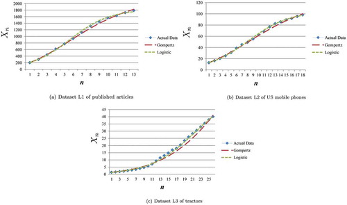
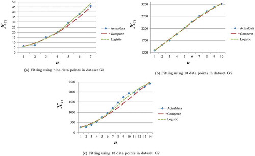
Six actual datasets were prepared for evaluation: three datasets (Kucharavy & Guio, 2015; Mar-Molinero, 1980; The World Bank, 2018) conform well to a logistic curve model, and the others (Bagchi, 1998; Franses, 1994a; Mitsuhashi, 1981) conform well to a Gompertz curve model. Dataset L1 of published articles (Kucharavy & Guio, 2015), dataset L2 of US mobile phones (The World Bank, 2018), and dataset L3 of tractors (Mar-Molinero, 1980) conform well to the logistic curve model as shown in Figure 1(a–c). Datasets L1, L2, and L3 contained 13, 18, and 26 data points, respectively.

Figure 1. Actual datasets that conform well to logistic curve model.

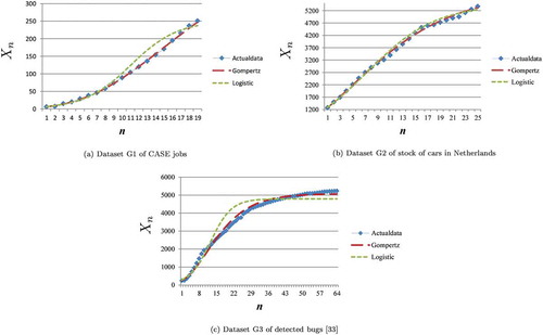
Dataset G1 of computer-aided software engineering (CASE) jobs (Bagchi, 1998), dataset G2 of stock of cars in Netherlands from 1965 to 1989 (Franses, 1994a), and dataset G3 of detected bugs (Mitsuhashi, 1981) conform well to the Gompertz curve model as shown in Figure 2(a–c). Datasets G1, G2, and G3 contained 19, 25, and 64 data points, respectively.

Figure 2. Actual datasets that conform well to Gompertz curve model.

4.2. Measure C

Determining the more appropriate model at an earlier stage is desirable because forecasting at an earlier stage is more valuable. Thus, the proposed model selection was applied to the first $n$ data points for each dataset to evaluate at how early a stage it was able to determine the more appropriate model.

Values of measure C were calculated only when all estimated parameters met their conditions (18), (19), (20), (32), (33), and (34). Not all estimated parameters always met their conditions for actual datasets. All estimated parameters for datasets L1, L2, and G2 met the conditions for all data, and those for dataset L3, G1, and G3 met the conditions except for $n=5,6,8,\dots ,16$, $n=4$ and $n=5$, and $n=4,\dots ,7$, respectively.

Values of measure C were calculated for the first $n$ data points in datasets L1, L2, and L3 as shown in Figure 3(a–c). The proposed model selection determined that the logistic model was more appropriate than the Gompertz model for dataset L1 except for $n=8,9,10$, dataset L2 except for $n=4,5,6$ and $n=12,13,14$, and dataset L3 for all $n$. The logistic model was actually more appropriate for all available data ($n=13,18$, and $26$ for dataset L1, L2, and L3) as shown in Figure 1(a–c).

Figure 3. Measure C using first $n$ data points for datasets L1, L2, and L3.

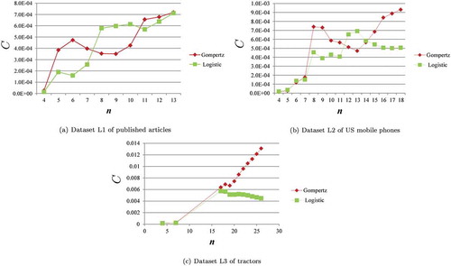
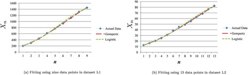
Moreover, the proposed model selection also determined that the Gompertz model was more appropriate than the logistic model when available data were the first 8, 9, and 10 data points in dataset L1 and the first 4, 5, 6, 12, 13, and 14 data points in dataset L2. Both models were compared with actual data using the first 9 data points in dataset L1 in Figure 4(a) and the first 13 data points in dataset L2 in Figure 4(b) because the difference between the two values of measure C was the largest for $n=8,9,10$ in dataset L1 and for $n=12,13,14$ in dataset L2. The Gompertz model looks more appropriate than the logistic model from the results of the proposed model selection.

Figure 4. Case of Gompertz model as more appropriate model.

Values of measure C were calculated for the first $n$ data points in datasets G1, G2, and G3 as shown in Figure 5(a–c). The proposed model selection determined that the Gompertz model was more appropriate than the logistic model for dataset G1 except for $n=6,7,8,9$, dataset G2 except for $n=7,8,9,10,11$, and dataset G3 except for $n=4,7,8,\dots ,25$. Actually, the Gompertz model was more appropriate for all available data ($n=19,25$, and $64$ for dataset G1, G2, and G3) as shown in Figure 2(a–c).

Figure 5. Measure C using first $n$ data points for datasets G1, G2, and G3.

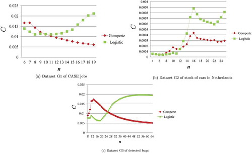
On the other hand, the proposed model selection also determined that the logistic model was more appropriate than the Gompertz model when available data were the first 6, …, 9 data points in dataset G1, the first 7, …, 11 data points in dataset G2, and the first 8, …, 25 data points in dataset G3. Both models were compared with actual data using the first 7 data points in dataset G1 in Figure 6(a), the first 10 data points in dataset G2 in Figure 6(b), and the first 14 data points in dataset G3 in Figure 6(c) because the difference between the two values of measure C was the largest for $n=6,\dots ,9$ in dataset G1, $n=7,\dots ,11$ in dataset G2, and $n=8,\dots ,25$ in dataset G3. The logistic model looks more appropriate than the Gompertz model from the results of the proposed model selection.

Figure 6. Case of Gompertz model as more appropriate model.

4.3. Stability of estimated saturation level

Estimated saturation level (parameter $k$) for actual data changes as available data points increase even though it never changes in exact solution data. However, if parameter $k$ is estimated by the more appropriate model, the estimated values must be more stable than values estimated by the less appropriate model when data points increase. If the range of $k$ estimated by the more appropriate model determined by the proposed model selection is smaller than that estimated by the less appropriate model, the proposed model selection determines the more appropriate model correctly.

Table 5 shows the range of estimated $k$ in the last stage where a more appropriate model was fixed because the results of the proposed model selection did not change in the stage for all actual datasets. The values of the range were calculated using the first $n=11,12,13$ data points for dataset L1, the first $n=15,\dots ,18$ data points for dataset L2, the first $n=17,\dots ,26$ data points for dataset L3, the first $n=10,\dots ,19$ data points for dataset G1, the first $n=13,\dots ,25$ data points for dataset G2, and the first $n=26,\dots ,64$ data points for dataset G3. The range of parameter $k$ estimated by the more appropriate model was smaller than that estimated by the less appropriate model as shown in Table 5. Therefore, the proposed model selection determined the more appropriate model correctly.

Table 5. Range of estimated $k$

Dataset	Appropriate	Range
	Model	Logistic	Gompertz
L1	Logistic	67.65	73.43
L2	Logistic	2.025	11.90
L3	Logistic	21.07	9.725E + 8
G1	Gompertz	124.3	75.81
G2	Gompertz	867.0	815.0
G3	Gompertz	1145	262.1

5. Conclusion

A model selection method has been proposed to select among growth curve models that have the same number of parameters. The key of the model selection method is to use integrable difference equations for the growth curve models and a measure of the mean relative squared error between actual data and estimates. The integrable difference equations have exact solutions that are on exact solutions of growth curve models and perfectly reproduce the parameter estimates from exact solution data. The ordinary forward or central difference equations cannot be used for model selection because they cannot reproduce estimates even from exact solution data. They produce the error between estimates and exact solution data. The measure of the mean relative squared error between actual data and estimates is suitable for model selection because it gives the same weight at every stage. The mean squared error, which is commonly used, gives too much weight at a later stage of bigger data, so it is not suitable for model selection. The proposed model selection method has been verified with six actual datasets when logistic and Gompertz curve models were chosen as alternatives of the growth curve models. Three datasets conform well to the logistic curve model, and the others to the Gompertz curve model. The more appropriate model alters in accordance with changes depending on available data points for actual data because actual data include noise. The proposed model selection determines the more appropriate model depending on available data points. Parameters estimated by the more appropriate model must be more stable than ones estimated by the less appropriate model when available data points increase. The range of saturation level parameters estimated by the more appropriate model determined by the proposed model selection is smaller than that estimated by the less appropriate model. Therefore, the proposed model selection determined the more appropriate model correctly.

Additional information

Funding

The author received no direct funding for this research.

Notes on contributors

Daisuke Satoh

Daisuke Satoh received his B.E. and M.E. degrees in electronics and communication engineering in 1992 and 1994 and his Ph.D. in information and computer science in 2002 from Waseda University, Tokyo, Japan. He joined NTT in 1994. He is currently working as a senior research engineer at NTT Network Technology Laboratories. His research interests include applied discrete systems, software reliability, and teletraffic issues. He received the Best Author Award from JSIAM in 2011 and the Best Presentation Award at the 79th annual Convention of the Japanese Psychological Association in 2016. Dr. Satoh is a member of JSIAM, ORSJ, and IEICE.

References

- Aggrey, S. (2002). Comparison of three nonlinear and spline regression models for describing chicken growth curves. Poultry Science, 81, 1782–17. doi:10.1093/ps/81.12.1782
- Bagchi, K. (1998). A model –Based study of CASE adoption and diffusion, in advanced computer system design (261–280). In K. B. Georege, W. Zobrist, & K. Trivedi eds. chap. 13. Amsterdam: Gordon and Breach Science Publishers.
- Bass, F. M. (1969). A new product growth for model consumer durables. Management Science, 15, 215–227. doi:10.1287/mnsc.15.5.215
- Bemmaor, A. C. (1992). Modeling the diffusion of new durable goods: Word-of-month effect versus consumer heterogeneity. In G. L. L. G. Laurent & B. Pras Eds., Research traditions in marketing. (Vol. 5, 201–223). chap. 6, Springer. Dordrecht: International Series in Quantiative Marketing.
- Chu, W. L., Wu, F. S., Kao, K. S., & Yen, D. C. (2009). Diffusion of mobile telephony: An empirical study in Taiwan. Telecommunications Policy, 33, 506–520. doi:10.1016/j.telpol.2009.07.003
- Çinlar, E. (1975). Introduction to stochastic process. Englewood Cliffs, NJ: Prentice-Hall.
- Franses, P. H. (1994a). Fitting a Gompertz curve. Journal of the Operational Reasearch Society, 45, 109–113. doi:10.1057/jors.1994.11
- Franses, P. H. (1994b). A method to select between Gompertz and logistic trend curves. Technological Forecasting & Social Change, 46, 45–49. doi:10.1016/0040-1625(94)90016-7
- Gregg, J., Hossel, C., & Richardson, J. (1964). Mathematical trend curves, an aid to forecasting. In Monograph No.1, Mathematical trend curves: An aid to forecasting (Vol. 1). Edinburgh: Oliver & Boyd.
- Gupta, R., & Jain, K. (2012). Diffusion of mobile telephony in India: An empirical study. Technological Forecasting & Social Change, 79, 709–715. doi:10.1016/j.techfore.2011.08.003
- Guseo, R., & Guidolin, M. (2009). Modelling a dynamic market potential: A class of automata networks for diffusion of innovations. Technological Forecating & Social Change, 76, 806–820. doi:10.1016/j.techfore.2008.10.005
- Hirota, R. (1979). Nonlinear partial difference equations. V. nonlinear equations reducible to linear equations. Journal of the Physical Society of Japan, 46, 312–319. doi:10.1143/JPSJ.46.312
- Hirota, R. (2000). Lecture on discrete equations. Saiensu-sha. in Japanese.
- Hirota, R., & Takahashi, D. (2003). Discrete and ultradiscrete systems. Kyoritsu Shuppan. in Japanese.
- Knízetová, H., Hyánek, J., Kníze, B., & Roubícek, J. (1991). Analysis of growth curve of fowl. I. chickens. British Poultry Science, 32, 1027–1038. doi:10.1080/00071669108417424
- Kucharavy, D., & Guio, R. D. (2015). Application of logistic growth curve. Procedia Engineering, 131, 280–290. doi:10.1016/j.proeng.2015.12.390
- Lechman, E. (2015). ICT diffusion in developing countries: Towards a new concept of technological takeoff. Switzerland: Springer International Publishing.
- Li, T. Y., & Yorke, J. A. (1975). Period three implies chaos. The American Mathematical Monthly, 82, 985–992. doi:10.1080/00029890.1975.11994008
- Mar-Molinero, C. (1980). Tractors in Spain: A logistic analysis. Journal of the Operatinal Resaerch Society, 31, 141–152. doi:10.1057/jors.1980.24
- Martino, J. P. (2003). A review of selected recent advances in technological forecasting. Technological Forecasting & Social Change, 70, 719–733. doi:10.1016/S0040-1625(02)00375-X
- Meade, N. (1984). The use of growth curves in forecasting market developemnt – a review and appraisal. Journal of Forecasting, 3, 429–451. doi:10.1002/for.3980030406
- Meade, N., & Islam, T. (1995). Forecasting with growth curves: An empirical, Internatinal. Journal of Forecasting, 11, 119–215.
- Mitsuhashi, T. (1981). Software quality assurance: Approach to statistical control. JUSE. in Japanese.
- Morisita, M. (1965). The fitting of the logistic equation to the rate of increase of population density. Researches on Population Ecology, 7, 52–55. doi:10.1007/BF02518815
- Narinc, D., Karaman, E., Firat, M. Z., & Aksoy, T. (2010). Comparison of non-linear growth models to describe the growth in Japanese quail. Journal of Animal and Veterinary Advances, 9, 1961–1966. doi:10.3923/javaa.2010.1961.1966
- Nguimkeu, P. (2014). A simple selection test between the Gompertz and logistic growth models. Technological Forecasting & Social Changes, 88, 98–105. doi:10.1016/j.techfore.2014.06.017
- Roush, W., & Branton, S. (2005). A comparison of fitting growth models with a genetic algorithm and nonlinear regression. Poultry Science, 84, 494–502. doi:10.1093/ps/84.3.494
- Satoh, D. (2000). A discrete Gompertz equation and a software reliability growth model. IEICE Transactions, E83-D. 1508–1513.
- Satoh, D. (2001). A discrete Bass model and its parameter estimation. Journal of the Operations Research Society of Japan, 44, 1–18. doi:10.15807/jorsj.44.1
- Satoh, D. (2019). Properties of Gompertz data revealed with non-Gompertz integrable difference equation. Cogent Mathematics & Statistics (to Appear), 6, 1. doi:10.1080/25742558.2019.1596552
- Satoh, D., & Matsumura, R. (2019). Monotonic decrease of upper limit estimated using Gompertz model with data described using logistic model, Japan. Journal of Industrial and Applied Mathematics, 36, 79–96. doi:10.1007/s13160-018-0333-9
- Satoh, D., & Uchida, M. (2010). Computer worm model describing infection via e-mail. Bulletin of the Japan Society for Industrial and Applied Mathematics, 20, 50–53. in Japanese.
- Satoh, D., & Yamada, S. (2001). Discrete equations and software reliability growth models, Proceedings of 12th International Symposium on software Reliability Engineering (pp. 176–184). Hong Kong.
- Satoh, D., & Yamada, S. (2002). Parameter estimation of discrete logistic curve models for software reliability assessment, Japan. Journal of Industrial and Applied Mathematics, 19, 39–53. doi:10.1007/BF03167447
- Skellam, J. G. (1951). Random dispersal in theoretical populations. Biometrika, 38(1/2 ), 196–218.
- The World Bank. (2018). Mobile cellular subscriptions per 100 people. Retrieved from http://databank.worldbank.org/data/country/USA/556d8fa6/Population_countries
- Ushiki, S. (1982). Central difference scheme and chaos. Physica D. Nonlinear Phenomena, 4, 407–424. doi:10.1016/0167-2789(82)90044-6
- Vieira, S., & Hoffmann, R. (1977). Comparison of the logistic and the Gompertz growth functions considering additive and multiplicative error terms. Applied Statistics, 26, 143–148. doi:10.2307/2347021
- Yamada, S. (2014). Software reliability modeling fundamentals and applications. Japan: Springer.
- Yamada, S., Inoue, S., & Satoh, D. (2002). Statistical data analysis modeling based on difference equations for software reliability assessment. Transactions of the Japan Society for Industrial and Applied Mathematics, 12, 155–168. in Japanese.
- Yamada, S., & Tamura, Y. (2016). OSS reliability measurement and assessment. Switzerland: Springer International Publishing.
- Yamakawa, P., Rees, G. H., Salas, J. M., & Alva, N. (2013). The diffusion of mobile telephones: An empirical analysis for Peru. Telecommunications Policy, 37, 594–606. doi:10.1016/j.telpol.2012.12.010
- Young, P., & Ord, J. (1989). Model selection and estimation for technology growth curves. International Journal of Forecasting, 5, 501–513. doi:10.1016/0169-2070(89)90005-8