Chen-G class of distributions

Abstract

The quest to generate distributions with more desirable and flexible properties for the modeling of data has led to an intense focus on the development of new families that are generalizations of existing distributions by researchers. A new family of distributions called the chen generated family is developed in this study. Its statistical properties such as the quantile, moments, incomplete moments, stochastic ordering and order statistics are derived by using the method of maximum likelihood, estimators for the parameters of the new family are developed. Three special distributions, Chen Burr III, Chen Kumaraswamy and Chen Weibull, are proposed from the new family, though it can generalize other distributions. A demonstration of the usefulness of the new family is performed using real dataset.

Keywords:

• Chen
• Weibull
• distribution
• moments
• stochastic ordering
• quantile

Jel:

• 62e15
• 60e05

PUBLIC INTEREST STATEMENT

Modeling of natural phenomena such as earthquakes, rainfall, tsunami and so on mostly involves the use of statistical distributions. Since the accuracy of the results largely depends on how well the distribution fits the dataset, the study develops a new family of distributions which is to improve the flexibility of existing distributions.

Conflict of Interest

The authors declare that there are no conflicts of interest regarding the publication of this article.

1. Introduction

The accuracy of parametric statistical inference and modeling of datasets largely depends on how well the probability distribution fits the given dataset once it has met all distributional assumptions. Several studies have been carried out on statistical distributions in the quest to generate distributions with more desirable and flexible properties that can model real-life datasets of varying shapes of density and failure rate functions. Currently, most studies are focused on developing new families that are generalizations of existing distributions to provide better fit to the modeling of data. These families of distributions are constructed by either compounding two or more distributions or adding one or more parameters to the baseline model. Many authors have extensively reviewed the various families of distributions (Hamedani, Yousof, Rasekhi, Alizadeh, & Najibi, 2018; Lee, Famoye, & Alzaatreh, 2013; Nasiru, 2018; Nasiru, Mwita, & Ngesa, 2018; Zubair, 2018).

In this study a new class of distributions is developed and proposed using the T-X approach (Alzaatreh, Lee, & Famoye, 2013). The Chen generated (CG) family of distributions is obtained by compounding the two-parameter Chen distribution (Chen, 2000) and an arbitrary baseline cumulative distribution function (cdf) of a continuous random variable. The main motivation for developing this family is to improve the flexibility of the existing classical distributions, thus to enabling them to provide a better fit to real data sets than other candidate distributions with the same number of parameters and model different kinds of failure rate (monotonic and non-monotonic).

The remaining sections of the paper follow this order: the Chen generated (CG) family of distributions is defined in section 2. The mixture representation of the probability density function (pdf) is presented in section 3. Some statistical properties of the family of distributions are derived in section 4. The estimators for the parameters of the family are developed in section 5. Some special distributions from the CG family of distributions are proposed and discussed in section 6. Simulations to examine the properties of estimators of parameters of the special distributions are carried out in section 7. Real-life data set is used to demonstrate the application of the special distributions in section 8. Concluding remarks of the study are captured in section 9.

2. Chen generated a family of distributions

Let $T$ be a Chen distributed continuous random variable, its cdf denoted by $F(t)$ is given by $F(t)=1-e^{\lambda \left(1-e^{t^{\beta }}\right)},t>0$ (Chen, 2000). Also, let $G(x)$and $g(x)$ be the respective cdf and pdf of an arbitrary continuous random variable $X$. The cdf of the CG family is defined as;

(1) $F(x)=\underset{0}{\overset{G(x)}{\int }}f(t)dt=A\left[1-e^{\lambda \left(1-e^{G{(x)}^{\beta }}\right)}\right],x>0,\lambda >0,\beta >0,$(1)

where $A=1/1-e^{\lambda \left(1-e\right)}$ is a normalizing constant, $\lambda$ and $\beta$ are scale and shape parameters, respectively. The pdf $f(x)$ of the family is given by;

(2) $f(x)=A\lambda \beta g(x)G(x{)}^{\beta -1}{e}^{G{(x)}^{\beta }}{e}^{\lambda \left(1-e^{G{(x)}^{\beta }}\right)},x>0,\lambda >0,\beta >0.$(2)

The survival function, $S(x)$of the CG family is;

(3) $S(x)=1-A\left[1-e^{\lambda \left(1-e^{G{(x)}^{\beta }}\right)}\right],x>0,\lambda >0,\beta >0.$(3)

The failure rate or hazard function, $h(x)$of the family is obtained as follows:

(4) $h(x)=\frac{A\lambda \beta g(x)G{(x)}^{\beta -1}{e}^{G{(x)}^{\beta }}{e}^{\lambda \left(1-e^{G{(x)}^{\beta }}\right)}}{1-A\left[1-e^{\lambda \left(1-e^{G{(x)}^{\beta }}\right)}\right]},x>0,\lambda >0,\beta >0.$(4)

3. Mixture representation of distribution

Mixture representation plays a useful role in the derivation of the statistical properties of the new family of distributions. Hence, the mixture representation of the pdf of the CG family of distributions is derived in this section.

By applying Taylor series expansion, the pdf of the CG family in Equation (2)(2) $f(x)=A\lambda \beta g(x)G(x{)}^{\beta -1}{e}^{G{(x)}^{\beta }}{e}^{\lambda \left(1-e^{G{(x)}^{\beta }}\right)},x>0,\lambda >0,\beta >0.$(2) is expressed as

(5) $f(x)=A\lambda \beta e^{\lambda }g(x)G(x{)}^{\beta -1}\sum _{i=0}^{\mathrm{\infty }}\sum _{j=0}^{\mathrm{\infty }}\frac{{(-1)}^i{\lambda }^i}{i!}\frac{{(i+1)}^j}{j!}G{(x)}^{\beta (j+1)-1}.$(5)

Equation (5)(5) $f(x)=A\lambda \beta e^{\lambda }g(x)G(x{)}^{\beta -1}\sum _{i=0}^{\mathrm{\infty }}\sum _{j=0}^{\mathrm{\infty }}\frac{{(-1)}^i{\lambda }^i}{i!}\frac{{(i+1)}^j}{j!}G{(x)}^{\beta (j+1)-1}.$(5) can be rewritten as;

$f(x)=A\lambda \beta e^{\lambda }g(x)\sum _{i=0}^{\mathrm{\infty }}\sum _{j=0}^{\mathrm{\infty }}\frac{{(-1)}^i{\lambda }^i}{i!}\frac{{(i+1)}^j}{j!}{\left[1-(1-G(x))\right]}^{\beta (j+1)-1}.$

$f(x)$ is further expanded using the binomial series expansion $(1-z{)}^{a-1}=\sum _{k=0}^{\mathrm{\infty }}{(-1)}^k\left(\begin{array}{c}a-1\\ k\end{array}\right)z^k,$ $|z|<1$ for any real non-integer $a>0$ as follows:

$f(x)=A\lambda \beta e^{\lambda }g(x)\sum _{i=0}^{\mathrm{\infty }}\sum _{j=0}^{\mathrm{\infty }}\frac{{(-1)}^i{(i+1)}^j{\lambda }^i}{i!j!}{\sum _{k=0}^{\mathrm{\infty }}(-1)}^k\left(\begin{array}{c}\beta (j+1)-1\\ k\end{array}\right){\left(1-G(x)\right)}^k.$

Assuming $a$ an integer in the binomial expansion,

(6) $f(x)=A\lambda \beta \sum _{i=0}^{\mathrm{\infty }}\sum _{j=0}^{\mathrm{\infty }}\sum _{k=0}^{\mathrm{\infty }}\sum _{l=0}^k{\omega }_{ijkl}g(x){\left(G(x)\right)}^l,$(6)

where

${\omega }_{ijkl}=\frac{{(-1)}^{i+k+l}{(i+1)}^j{\lambda }^i{e}^{\lambda }}{i!j!}\left(\begin{array}{c}\beta (j+1)-1\\ k\end{array}\right)\left(\begin{array}{c}k\\ l\end{array}\right).$

From Equation (6)(6) $f(x)=A\lambda \beta \sum _{i=0}^{\mathrm{\infty }}\sum _{j=0}^{\mathrm{\infty }}\sum _{k=0}^{\mathrm{\infty }}\sum _{l=0}^k{\omega }_{ijkl}g(x){\left(G(x)\right)}^l,$(6) , the CG family’s density is expressed as a product of the parameters and the sum of the product of the pdf and weighted power series of the baseline distribution function $G(x)$.

Alternatively, Equation (6)(6) $f(x)=A\lambda \beta \sum _{i=0}^{\mathrm{\infty }}\sum _{j=0}^{\mathrm{\infty }}\sum _{k=0}^{\mathrm{\infty }}\sum _{l=0}^k{\omega }_{ijkl}g(x){\left(G(x)\right)}^l,$(6) can further be written in terms of the exponentiated-G (expo-G) density function as

(7) $f(x)=A\lambda \beta \sum _{i=0}^{\mathrm{\infty }}\sum _{j=0}^{\mathrm{\infty }}\sum _{k=0}^{\mathrm{\infty }}\sum _{l=0}^k{\omega }_{ijkl}^{\ast }{\pi }_{l+1}(x),$(7)

where ${{\omega }_{ijkl}}^{\ast }=\frac{{\omega }_{ijkl}}{l+1}$ and ${\pi }_{l+1}(x)=(l+1)g(x){\left(G(x)\right)}^l$ is the expo-G density function with the power parameter $(l+1)$.

4. Statistical properties

This section discusses some of the statistical properties of the CG family of distributions. These include: quantile function, non-central moments, moments, generating functions, inequality measures, entropies, residual life, stochastic ordering and order statistics.

4.1. Quantile function

Proposition 1. The quantile function for CG family of distributions is given by

(8) $Q_G(u)=x_u=G^{-1}{\left(ln\left[1-\frac{ln(1-u/A)}{\lambda }\right]\right)}^{\frac{1}{\beta }},0<u<1,$(8)

Proof. The quantile function $Q_G(u)$ of a random variable $X$ is defined as $F(x_u)=P(X\le x_u)=u,u\in (0,1)$. Replacing $x$ with $x_u$ in Equation (1)(1) $F(x)=\underset{0}{\overset{G(x)}{\int }}f(t)dt=A\left[1-e^{\lambda \left(1-e^{G{(x)}^{\beta }}\right)}\right],x>0,\lambda >0,\beta >0,$(1) , equating $F(x_u)$ to $u$ and making $x_u$ the subject yields the quantile function. The median of the family is obtained by substituting $u=0.5$ in Equation (8)(8) $Q_G(u)=x_u=G^{-1}{\left(ln\left[1-\frac{ln(1-u/A)}{\lambda }\right]\right)}^{\frac{1}{\beta }},0<u<1,$(8) .

4.2. Moments, moment generating functions and incomplete moments

Moments are very essential in statistical analysis as they can be used to study important features (such as tendencies, variation, skewness, kurtosis and so on) of a distribution.

4.2.1. Non-central moments

Proposition 2. The $r^{\mathrm{t}\mathrm{h}}$ non-central moment of the CG family is given by

(9) ${\mu }_r^{\prime }=A\lambda \beta \sum _{i=0}^{\mathrm{\infty }}\sum _{j=0}^{\mathrm{\infty }}\sum _{k=0}^{\mathrm{\infty }}\sum _{l=0}^k{\omega }_{ijkl}{\tau }_{(r,l)},r=1,2,...,$(9)

$\mathrm{w}\mathrm{h}\mathrm{e}\mathrm{r}\mathrm{e}{\tau }_{(r,l)}=\underset{-\mathrm{\infty }}{\overset{\mathrm{\infty }}{\int }}{x}^{r}g(x){\left(G(x)\right)}^{l}dx$ is the probability weighted moment of the baseline distribution $G(x).$

Proof. The $r^{\mathrm{t}\mathrm{h}}$ non-central moment is defined as $E(X^r)={\mu }_r^{\prime }=\underset{-\mathrm{\infty }}{\overset{\mathrm{\infty }}{\int }}{x}^{r}f(x)dx$, thus using the mixture form of the density, the $r^{\mathrm{t}\mathrm{h}}$ non-central moment of the CG family is given by ${\mu }_r^{\prime }=A\lambda \beta \sum _{i=0}^{\mathrm{\infty }}\sum _{j=0}^{\mathrm{\infty }}\sum _{k=0}^{\mathrm{\infty }}\sum _{l=0}^k{\omega }_{ijkl}\underset{-\mathrm{\infty }}{\overset{\mathrm{\infty }}{\int }}{x}^{r}g(x){\left(G(x)\right)}^{l}dx.$

Alternatively, the $r^{\mathrm{t}\mathrm{h}}$ non-central moment of the CG family can be described in terms of the quantile function as follows;

$\mathrm{L}\mathrm{e}\mathrm{t}G(x)=u,x=G^{-1}(u)=Q_G(u),\frac{dG(x)}{dx}=\frac{du}{dx}=g(x)\mathrm{a}\mathrm{n}\mathrm{d}g(x)dx=du$. From Equation (9)(9) ${\mu }_r^{\prime }=A\lambda \beta \sum _{i=0}^{\mathrm{\infty }}\sum _{j=0}^{\mathrm{\infty }}\sum _{k=0}^{\mathrm{\infty }}\sum _{l=0}^k{\omega }_{ijkl}{\tau }_{(r,l)},r=1,2,...,$(9) ,

(10) ${\mu }_r^{\prime }=A\lambda \beta \sum _{i=0}^{\mathrm{\infty }}\sum _{j=0}^{\mathrm{\infty }}\sum _{k=0}^{\mathrm{\infty }}\sum _{l=0}^k{\omega }_{ijkl}\underset{0}{\overset{1}{\int }}{Q}_G{(u)}^r{u}^{l}du.$(10)

4.2.2. Moment generating functions

Proposition 3. The moment generating function of the CG family is given by

(11) $M_X(t)=A\lambda \beta \sum _{i=0}^{\mathrm{\infty }}\sum _{j=0}^{\mathrm{\infty }}\sum _{k=0}^{\mathrm{\infty }}\sum _{r=0}^{\mathrm{\infty }}\sum _{l=0}^k\frac{{(t)}^r}{r!}{\omega }_{ijkl}{\tau }_{(r,l).}$(11)

Proof. By definition, the moment generating function is given by $M_X(t)=\underset{-\mathrm{\infty }}{\overset{\mathrm{\infty }}{\int }}{e}^{tx}f(x)dx$, expanding $M_X(t)$ using Taylor series, $M_X(t)=\sum _{r=0}^{\mathrm{\infty }}\frac{{(t)}^r}{r!}\underset{-\mathrm{\infty }}{\overset{\mathrm{\infty }}{\int }}{x}^{r}f(x)dx$.

But from Equation (9)(9) ${\mu }_r^{\prime }=A\lambda \beta \sum _{i=0}^{\mathrm{\infty }}\sum _{j=0}^{\mathrm{\infty }}\sum _{k=0}^{\mathrm{\infty }}\sum _{l=0}^k{\omega }_{ijkl}{\tau }_{(r,l)},r=1,2,...,$(9) , $\underset{-\mathrm{\infty }}{\overset{\mathrm{\infty }}{\int }}{x}^{r}f(x)dx=A\lambda \beta \sum _{i=0}^{\mathrm{\infty }}\sum _{j=0}^{\mathrm{\infty }}\sum _{k=0}^{\mathrm{\infty }}\sum _{l=0}^k{\omega }_{ijkl}{\tau }_{(r,l)},$ hence the proof.

Alternatively, letting $G(x)=u$, the moment generating function can be expressed in terms of quantile functions as;

(12) $M_X(t)=A\lambda \beta \sum _{i=0}^{\mathrm{\infty }}\sum _{j=0}^{\mathrm{\infty }}\sum _{k=0}^{\mathrm{\infty }}\sum _{l=0}^k{\omega }_{ijkl}\underset{0}{\overset{1}{\int }}{e}^{t{Q}_G(u)}{u}^{l}du.$(12)

4.2.3. Incomplete moments

Proposition 4. The $r^{th}$ incomplete moment of the CG family of distribution is given by

(13) $M_r(y)=A\lambda \beta \sum _{i=0}^{\mathrm{\infty }}\sum _{j=0}^{\mathrm{\infty }}\sum _{k=0}^{\mathrm{\infty }}\sum _{l=0}^k{\omega }_{ijkl}\underset{-\mathrm{\infty }}{\overset{y}{\int }}{x}^{r}g(x){\left(G(x)\right)}^{l}dx,r=1,2,....$(13)

Proof. The $r^{th}$ incomplete moment is defined as $M_r(y)=\underset{-\mathrm{\infty }}{\overset{y}{\int }}{x}^{r}f(x)dx.$ Substituting the mixture representation of the density function into the definition of the $r^{th}$ incomplete moments completes the proof.

Alternatively, letting $G(x)=u$, the incomplete moments can be expressed in terms of the quantile function as;

(14) $M_r(y)=A\lambda \beta \sum _{i=0}^{\mathrm{\infty }}\sum _{j=0}^{\mathrm{\infty }}\sum _{k=0}^{\mathrm{\infty }}\sum _{l=0}^k{\omega }_{ijkl}\underset{0}{\overset{G(y)}{\int }}{Q}_G{(u)}^r{u}^{l}du.$(14)

4.3. Inequality measures

Lorenz and Bonferroni curves are applied in so many fields such as econometrics, demography, reliability, medicine and insurance. They are generally used in studying inequality measures like income and poverty.

4.3.1. Lorenz curve

The Lorenz curve ${\mathrm{L}}_F(y)$ for incomplete moments is defined as ${\mathrm{L}}_F(y)=\frac{1}{\mu }\underset{-\mathrm{\infty }}{\overset{y}{\int }}xf(x)dx$ for the CG family, it is given by;

(15) ${\mathrm{L}}_F(y)=\frac{A\lambda \beta }{\mu }\sum _{i=0}^{\mathrm{\infty }}\sum _{j=0}^{\mathrm{\infty }}\sum _{k=0}^{\mathrm{\infty }}\sum _{l=0}^k{\omega }_{ijkl}\underset{-\mathrm{\infty }}{\overset{y}{\int }}xg(x){\left(G(x)\right)}^{l}dx.$(15)

Alternatively, letting $G(x)=u$, ${\mathrm{L}}_F(y)$ can be expressed in terms of the quantile functions as;

(16) ${\mathrm{L}}_F(y)=\frac{A\lambda \beta }{\mu }\sum _{i=0}^{\mathrm{\infty }}\sum _{j=0}^{\mathrm{\infty }}\sum _{k=0}^{\mathrm{\infty }}\sum _{l=0}^k{\omega }_{ijkl}\underset{0}{\overset{G(y)}{\int }}{Q}_G(u)u^{l}du$(16)

4.3.2. Bonferroni curve

Bonferroni curve $B_F(y)$ is defined as $B_F(y)=\frac{{\mathrm{L}}_F(y)}{F(y)}$, hence for the CG family it is given by;

(17) $B_F(y)=\frac{A\lambda \beta }{\mu F(y)}\sum _{i=0}^{\mathrm{\infty }}\sum _{j=0}^{\mathrm{\infty }}\sum _{k=0}^{\mathrm{\infty }}\sum _{l=0}^k{\omega }_{ijkl}\underset{-\mathrm{\infty }}{\overset{y}{\int }}xg(x){\left(G(x)\right)}^{l}dx.$(17)

4.4. Mean residual life

The mean residual life of a component (which is the average survival time of the component after it has exceeded a specific time$y$) is defined as $E(X-y/X>y).$

Proposition 5. The mean residual life of a CG random variable $Y$ is given by

(18) $\bar{M}(y)=\frac{1}{1-F(y)}\left[\mu -A\lambda \beta \sum _{i=0}^{\mathrm{\infty }}\sum _{j=0}^{\mathrm{\infty }}\sum _{k=0}^{\mathrm{\infty }}\sum _{l=0}^k{\omega }_{ijkl}\underset{-\mathrm{\infty }}{\overset{y}{\int }}xg(x){\left(G(x)\right)}^{l}dx\right]-y.$(18)

Proof. The mean residual life is defined as $\bar{M}(y)=\frac{1}{1-F(y)}\left[\mu -\underset{-\mathrm{\infty }}{\overset{y}{\int }}xf(x)dx\right]-y$. Substituting $f(x)$ in Equation (6)(6) $f(x)=A\lambda \beta \sum _{i=0}^{\mathrm{\infty }}\sum _{j=0}^{\mathrm{\infty }}\sum _{k=0}^{\mathrm{\infty }}\sum _{l=0}^k{\omega }_{ijkl}g(x){\left(G(x)\right)}^l,$(6) into $\bar{M}(y)$ gives the mean residual life.

4.5. Entropy

Entropy is a measure of variation or uncertainty of a random variable. Its application spans across probability theory, engineering and science in general.

4.5.1. Rényi’s entropy

The Rényi’s entropy (Rényi, 1961) for a random variable with pdf $f(x)$, is defined as;

${\mathrm{I}}_R(\delta )=\frac{1}{1-\delta }log\left[\underset{-\mathrm{\infty }}{\overset{\mathrm{\infty }}{\int }}{f}^{\delta }(x)dx\right],\delta \ne 1,\delta >0$

Proposition 5. Renyi’s entropy for the CG random variable is given by;

(19) ${\mathrm{I}}_R(\delta )=\frac{1}{1-\delta }log\left[{\left(A\lambda \beta \right)}^{\delta }\sum _{i=0}^{\mathrm{\infty }}\sum _{j=0}^{\mathrm{\infty }}\sum _{k=0}^{\mathrm{\infty }}\sum _{l=0}^k{\varpi }_{ijkl}\underset{-\mathrm{\infty }}{\overset{\mathrm{\infty }}{\int }}g{(x)}^{\delta }{\left(G(x)\right)}^{l}dx\right],\delta \ne 1,\delta >0,$(19)

where

${\varpi }_{ijkl}=\frac{{(-1)}^{i+k+l}{\left(\lambda \delta \right)}^i}{i!}\frac{{(i+\delta )}^j}{j!}{e}^{\lambda \delta }\left(\begin{array}{c}\beta (j+\delta )-1\\ k\end{array}\right)\left(\begin{array}{c}k\\ l\end{array}\right)$

Proof. From Equation (2)(2) $f(x)=A\lambda \beta g(x)G(x{)}^{\beta -1}{e}^{G{(x)}^{\beta }}{e}^{\lambda \left(1-e^{G{(x)}^{\beta }}\right)},x>0,\lambda >0,\beta >0.$(2) , $f^{\delta }(x)={\left(A\lambda \beta \right)}^{\delta }g(x{)}^{\delta }G(x{)}^{\delta \beta -1}{e}^{\delta G{(x)}^{\beta }}{e}^{\lambda \delta }{e}^{-\lambda \delta e^{G{(x)}^{\beta }}}$

Adopting similar concept for expanding the density, $f^{\delta }(x)$ becomes

$f^{\delta }(x)={\left(A\lambda \beta \right)}^{\delta }\sum _{i=0}^{\mathrm{\infty }}\sum _{j=0}^{\mathrm{\infty }}\sum _{k=0}^{\mathrm{\infty }}\sum _{l=0}^k{\varpi }_{ijkl}g{(x)}^{\delta }{\left(G(x)\right)}^l$

where ${\varpi }_{ijkl}=\frac{{(-1)}^{i+k+l}{\left(\lambda \delta \right)}^i}{i!}\frac{{(i+\delta )}^j}{j!}{e}^{\lambda \delta }\left(\begin{array}{c}\beta (j+\delta )-1\\ k\end{array}\right)\left(\begin{array}{c}k\\ l\end{array}\right)$. Substituting $f^{\delta }(x)$ into ${\mathrm{I}}_R(\delta )$ completes the proof.

4.6. Stochastic ordering

Ordering mechanism in data can easily be shown using stochastic ordering. Let $X$ and $Y$ be random variables with cdfs $F_X(x)$ and $F_Y(x)$ respectively. $X$ is less than $Y$ in likelihood ratio order $(X{\le }_{lr}Y)$, if the function $f(x)/g(x)\mathrm{i}\mathrm{s}\mathrm{d}\mathrm{e}\mathrm{c}\mathrm{r}\mathrm{e}\mathrm{a}\mathrm{s}\mathrm{i}\mathrm{n}\mathrm{g}\mathrm{f}\mathrm{o}\mathrm{r}\mathrm{a}\mathrm{l}\mathrm{l}x$.

Proposition 6. Let $X\text{~}CG({\lambda }_1,\beta ,\psi )$ and $Y\text{~}CG({\lambda }_2,\beta ,\psi )$, where $\psi$ is a $(p\times 1)$ vector of parameters associated with the baseline distribution. $X$ is less than $Y$ in likelihood ratio order $(X{\le }_{lr}Y)$ if ${\lambda }_2<{\lambda }_1$.

Proof. The ratio of their pdfs is given by $\frac{f_X(x)}{f_Y(x)}=\frac{{\lambda }_1}{{\lambda }_2}{e^{({\lambda }_1-{\lambda }_2)(1-}}^{e^{G{(x)}^{\beta }})}$, which is a decreasing function if ${\lambda }_2<{\lambda }_1$.

4.7. Order statistics

The pdf for the $p^{th}$ order statistic $X_{p:n}$, of an independent identically distributed random sample $X_1,X_2,...,X_n$ of size $n$,$f_{X_{p:n}}(x)$, is given by;

$f_{X_{p:n}}(x)=\frac{n!}{(p-1)!(n-p)!}{\left[F(x)\right]}^{p-1}{\left[1-F(x)\right]}^{n-p}f(x),p=1,2,\dots ,n.$

Expanding ${\left[F(x)\right]}^{p-1}$ using binomial expansion, ${\left[F(x)\right]}^{p-1}=\sum _{i=0}^{p-1}{{(-1)}^i\left(\begin{array}{c}p-1\\ i\end{array}\right)\left[1-F(x)\right]}^i$. Substituting into the density of the $p^{th}$ order statistic yields,

$f_{X_{p:n}}(x)=\frac{n!}{(p-1)!(n-p)!}\sum _{i=0}^{p-1}{(-1)}^i\left(\begin{array}{c}p-1\\ i\end{array}\right){\left[S(x)\right]}^{n-p+i}f(x)$

where ${\left[S(x)\right]}^{n-p+i}={\left[1-F(x)\right]}^{n-p+i}$.

Hence, the pdf for the $p^{th}$ order statistic is given by;

(20) $\begin{array}{rl}& f_{X_{p:n}}\left(x\right)=\frac{n!}{\left(p-1\right)!\left(n-p\right)!}\sum _{i=0}^{p-1}{\left(-1\right)}^i\left(\begin{array}{c}p-1\\ i\end{array}\right)A\lambda \beta g(x)G{\left(x\right)}^{\beta -1}{e}^{G{\left(x\right)}^{\beta }}\times e^{\lambda \left(n-p+i+1\right)\left(1-e^{G{(x)}^{\beta }}\right)}\end{array}$(20)

Employing a similar concept of expanding the density of the CG family, a mixture representation of the pdf of the $p^{th}$ order statistic is defined as;

(21) $f_{X_{p:n}}(x)=\frac{n!A\lambda \beta }{(p-1)!(n-p)!}\sum _{i=0}^{p-1}\sum _{j=0}^{\mathrm{\infty }}\sum _{k=0}^{\mathrm{\infty }}\sum _{l=0}^{\mathrm{\infty }}\sum _{m=0}^l{D}_{ijklm}g(x)G(x{)}^m,$(21)

where

$D_{ijkl}=\frac{{(-1)}^{i+j+l+m}{\left[\lambda (n-p+i+1)\right]}^j}{i!}\frac{{\left(j+1\right)}^k}{k!}\left(\begin{array}{c}p-1\\ i\end{array}\right)\left(\begin{array}{c}\beta (k+1)-1\\ l\end{array}\right)\left(\begin{array}{c}l\text{crm}\end{array}\right)e^{\lambda (n-p+i+1)}.$

4.7.1. Moments of order statistics

The $r^{th}$ non-central moment of the $p^{th}$ order statistic is given by $E(X_{p:n}^r)={\mu }_r^{\prime (p:n)}=\underset{-\mathrm{\infty }}{\overset{\mathrm{\infty }}{\int }}{x}^r{f}_{X_{p:n}}(x)dx$. Substituting Equation (21)(21) $f_{X_{p:n}}(x)=\frac{n!A\lambda \beta }{(p-1)!(n-p)!}\sum _{i=0}^{p-1}\sum _{j=0}^{\mathrm{\infty }}\sum _{k=0}^{\mathrm{\infty }}\sum _{l=0}^{\mathrm{\infty }}\sum _{m=0}^l{D}_{ijklm}g(x)G(x{)}^m,$(21) into $E(X_{p:n}^r),$ the $r^{th}$ non-central moment of the $p^{th}$ order statistic of the CG random variable is given by,

(22) $E(X_{p:n}^r)=\frac{n!A\lambda \beta }{(p-1)!(n-p)!}\sum _{i=0}^{p-1}\sum _{j=0}^{\mathrm{\infty }}\sum _{k=0}^{\mathrm{\infty }}\sum _{l=0}^{\mathrm{\infty }}\sum _{m=0}^l{D}_{ijklm}{\tau }_{(r,m)}$(22)

where ${\tau }_{(r,m)}=\underset{-\mathrm{\infty }}{\overset{\mathrm{\infty }}{\int }}{x}^{r}g(x)G{(x)}^{m}dx$ is the probability weighted moment of the baseline distribution.

5. Parameter estimation

Maximum likelihood estimation method was used in estimating the parameters for the family of distribution for similar reasons as stated in Nasiru et al. (Nasiru et al., 2018). Given a random sample $x_1,x_2,...,x_n$ of size $n$ from the CG family of distributions, the total log-likelihood function is given by

(23) $\begin{array}{c}\mathrm{\ell }=nlogA\lambda \beta +\sum _{i=1}^{n}logg(x_i;\psi )+(\beta -1)\sum _{i=1}^{n}logG(x_i;\psi )+\sum _{i=1}^{n}G{(x_i;\psi )}^{\beta }+\lambda \sum _{i=1}^n\left(1-e^{G{(x_i;\psi )}^{\beta }}\right),\end{array}$(23)

where $\psi$ is a $(p\times 1)$ vector of parameters associated with the baseline distribution.

The parameters are then estimated by partially differentiating the total log-likelihood function with respect to the parameters of the CG family as follows.

(24) $\frac{\mathrm{\partial }\mathrm{\ell }}{\mathrm{\partial }\lambda }=\frac{n}{\lambda }+\frac{n(1-e)e^{\lambda (1-e)}}{1-e^{\lambda (1-e)}}+\sum _{i=1}^n(1-e^{G{(x_i;\psi )}^{\beta }}),$(24)

(25) $\begin{array}{c}\frac{\mathrm{\partial }\mathrm{\ell }}{\mathrm{\partial }\beta }=\frac{n}{\lambda }+\sum _{i=1}^{n}logG(x_i;\psi )+\sum _{i=1}^{n}G{(x_i;\psi )}^{\beta }logG(x_i;\psi )-\lambda \sum _{i=1}^{n}G{(x_i;\psi )}^{\beta }{e}^{G{(x_i;\psi )}^{\beta }}logG(x_i;\psi )\end{array}$(25)

and

(26) $\begin{array}{rl}& \frac{\mathrm{\partial }\mathrm{\ell }}{\mathrm{\partial }\psi }=\sum _{i=1}^n\frac{g_k^{\prime }(x_i;\psi )}{G(x_i;\psi )}+(\beta -1)\sum _{I=1}^n\frac{G_k^{\prime }(x_i;\psi )}{G(x_i;\psi )}+\sum _{i=1}^n{G}_K^{\prime }(x_i;\psi )G{(x_i;\psi )}^{\beta -1}-\lambda \beta \sum _{i=1}^n{G}_K^{\prime }(x_i;\psi )G{(x_i;\psi )}^{\beta -1}{e}^{G{(x_i;\psi )}^{\beta }},\end{array}$(26)

where $g_K^{\prime }(x_i;\psi )=\frac{\mathrm{\partial }g(x_i;\psi )}{\mathrm{\partial }\psi }$ and $G_K^{\prime }(x_i;\psi )=\frac{\mathrm{\partial }G(x_i;\psi )}{\mathrm{\partial }\psi }$.

Equating the score functions to zero and numerically solving the system of equations using techniques such as the quasi Newton-Raphson method, gives the maximum likelihood estimates for the parameters. The interval estimates of the parameters are obtained by first finding the observed $(p\times p)$ information matrix given by $J(\vartheta )=\frac{{\mathrm{\partial }}^2\mathrm{\ell }}{\mathrm{\partial }q\mathrm{\partial }r}$ (for $q,r=\lambda ,\beta ,\psi$ and $\vartheta =(\lambda ,\beta ,\psi {)}^T$), whose elements can be numerically computed. Under the regularity conditions, as $n\to \mathrm{\infty }$, ${\hat{\vartheta }}_{}{N}_p(0,J(\hat{\vartheta }{)}^{-1})$, where $J(\hat{\vartheta })$ is the observed information matrix evaluated at $\hat{\vartheta }.$ The approximate$100(1-\rho )\mathrm{\%}$ confidence intervals (where $\rho$ is the significance level) can be constructed using the asymptotic normal distribution.

6. Some special distributions

The CG family of distributions can be used to extend many distributions to create more flexibility in their applications. In this section some special distributions were developed.

6.1. Chen Burr III distribution

Suppose that the baseline distribution is Burr III (Burr, 1942), it’s cdf and pdf are given by $G(x)={\left(1+x^{-\theta }\right)}^{-\gamma }$ and $g(x)=\gamma \theta x^{-\theta -1}{\left(1+x^{-\theta }\right)}^{-\gamma -1}$, $x>0,\theta >0,\gamma >0$ respectively. The cdf of Chen Burr III (CB) is given by

(27) $F(x)=A\left[1-exp\left(\lambda \left(1-e^{{\left(1+x^{-\theta }\right)}^{-\gamma \beta }}\right)\right)\right],x>0,\alpha >0,\beta >0,\gamma >0,\lambda >0.$(27)

Its corresponding density and hazard functions are, respectively

(28) $f(x)=A\lambda \beta \gamma \theta {\left(x\right)}^{-\theta -1}{\left(1+x^{-\theta }\right)}^{-\gamma \beta -1}exp\left[{\left(1+x^{-\theta }\right)}^{-\gamma \beta }+\lambda \left(1-e^{{\left(1+x^{-\theta }\right)}^{-\gamma \beta }}\right)\right],x>0$(28)

and

(29) $h(x)=\frac{A\lambda \beta \gamma \theta {\left(x\right)}^{-\theta -1}{\left(1+x^{-\theta }\right)}^{-\gamma \beta -1}exp\left[{\left(1+x^{-\theta }\right)}^{-\gamma \beta }+\lambda \left(1-e^{{\left(1+x^{-\theta }\right)}^{-\gamma \beta }}\right)\right]}{1-A\left[1-exp\lambda \left(1-e^{{\left(1+x^{-\theta }\right)}^{-\gamma \beta }}\right)\right]},x>0.$(29)

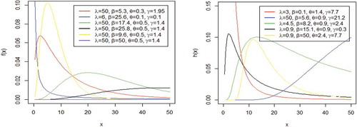
Plots of the density and hazard rate functions of the CB distribution are displayed in Figure 1. The density plot exhibit varying shapes including unimodal with different degrees of kurtosis, right skewed and reversed J shapes. The hazard rate function for some selected values exhibited upside down bathtub, decreasing and increasing failure rates.

Figure 1. Plots of density and hazard rate functions of CB distribution

The CB distribution’s quantile function $Q_G(u)$ is given by;

$Q_G(u)=x_u={\left[{\left(log\left(1-\left(\frac{log\left(1-u/A\right)}{\lambda }\right)\right)\right)}^{-\frac{1}{\gamma \beta }}-1\right]}^{-\frac{1}{\theta }}.$

6.2. Chen Kumaraswamy distribution

The Chen Kumaraswamy (CK) distribution uses the Kumaraswamy distribution (Kumaraswamy, 1980) with pdf and cdf respectively given by $G(x)=1-{\left(1-x^a\right)}^b$ and $g(x)=ab{x}^{a-1}{\left(1-x^a\right)}^{b-1}$, $0<x<1,a>0,b>0$ as the baseline distribution. The cdf of CK distribution is given by

(30) $F(x)=A\left[1-exp\lambda \left[1-e^{{\left[1-{\left(1-x^a\right)}^b\right]}^{\beta }}\right]\right]x>0,a>0,b>0,\beta >0,\lambda >0,$(30)

with its corresponding density and hazard rate functions, respectively, given by

(31) $\begin{array}{rl}& f(x)=A\lambda \beta ab{x}^{a-1}{\left(1-x^a\right)}^{b-1}{\left(1-{\left(1-x^a\right)}^b\right)}^{\beta -1}exp\left[{\left(1-{\left(1-x^a\right)}^b\right)}^{\beta }+\lambda \left(1-e^{{\left(1-{\left(1-x^a\right)}^b\right)}^{\beta }}\right)\right],x>0\end{array}$(31)

and

(32) $\begin{array}{rl}& h(x)=\frac{A\lambda \beta ab{x}^{a-1}{\left(1-x^a\right)}^{b-1}{\left(1-{\left(1-x^a\right)}^b\right)}^{\beta -1}exp\left[{\left(1-{\left(1-x^a\right)}^b\right)}^{\beta }+\lambda \left(1-e^{{\left(1-{\left(1-x^a\right)}^b\right)}^{\beta }}\right)\right]}{1-\left[1-exp\lambda \left[1-e^{{\left[1-{\left(1-x^a\right)}^b\right]}^{\beta }}\right]\right]},x>0.\end{array}$(32)

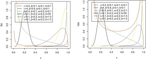
Plots of the density and hazard rate functions of the CK distribution are displayed in Figure 2. The plot of the density shows shapes such as; the reversed J, left skewed, right skewed and unimodal shapes among others. The hazard rate plot for some selected values exhibits increasing and decreasing failure rates, unimodal and bathtub shapes.

Figure 2. Plots of the density and hazard rate function of CK distribution

The quantile function $Q_G(u)$ is obtained as.

$Q_G(u)=x_u={\left[1-{\left(1-{\left(log\left(1-\left(\frac{log\left(1-u/A\right)}{\lambda }\right)\right)\right)}^{\frac{1}{\beta }}\right)}^{\frac{1}{b}}\right]}^{\frac{1}{a}}$

6.3. Chen Weibull distribution

Chen Weibull (CW) distribution is obtained using Weibull distribution (Weibull, 1951) with cdf and pdf, respectively, given by $G(x)=1-e^{-{\left(\frac{x}{\alpha }\right)}^{\gamma }}$ and $g(x)=\left(\frac{\gamma }{\alpha }\right){\left(\frac{x}{\alpha }\right)}^{\gamma -1}{e}^{-{\left(\frac{x}{\alpha }\right)}^{\gamma }}$as baseline distribution. The cdf and pdf of the CW distribution are, respectively, given by

(33) $F(x)=A\left[1-exp\lambda \left[1-e^{{\left(1-e^{-{\left(\frac{x}{\alpha }\right)}^{\gamma }}\right)}^{\beta }}\right]\right],x>0,\alpha >0,\beta >0,\lambda >0,\gamma >0$(33)

and

(34) $\begin{array}{rl}& f(x)=A\lambda \beta \left(\frac{\gamma }{\alpha }\right){\left(\frac{x}{\alpha }\right)}^{\gamma -1}{\left(1-e^{-{\left(\frac{x}{\alpha }\right)}^{\gamma }}\right)}^{\beta -1}exp\left[\lambda {\left(1-e^{-{\left(\frac{x}{\alpha }\right)}^{\gamma }}\right)}^{\beta }-{\left(\frac{x}{\alpha }\right)}^{\gamma }+\left(1-e^{-{\left(\frac{x}{\alpha }\right)}^{\gamma }}\right)\right],x>0.\end{array}$(34)

The hazard rate function is given by

(35) $\begin{array}{rl}& h(x)=\frac{A\lambda \beta \left(\frac{\gamma }{\alpha }\right){\left(\frac{x}{\alpha }\right)}^{\gamma -1}{\left(1-e^{-{\left(\frac{x}{\alpha }\right)}^{\gamma }}\right)}^{\beta -1}exp\left[\lambda {\left(1-e^{-{\left(\frac{x}{\alpha }\right)}^{\gamma }}\right)}^{\beta }-{\left(\frac{x}{\alpha }\right)}^{\gamma }+\left(1-e^{-{\left(\frac{x}{\alpha }\right)}^{\gamma }}\right)\right]}{1-A\left[1-exp\lambda \left[1-e^{{\left(1-e^{-{\left(\frac{x}{\alpha }\right)}^{\gamma }}\right)}^{\beta }}\right]\right]},x>0.\end{array}$(35)

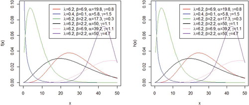
The CW distribution’s plots of its density exhibit; right skewed, left skewed, unimodal and reversed J shapes among others as shown in Figure 3. The hazard rate plot of the CW distribution for some selected values exhibits varying shapes such as increasing and decreasing failure rates, right and left skewed unimodal shapes and upside down bathtub shape.

Figure 3. Plots of density and hazard rate function of CW distribution

The quantile function $Q_G(u)$ of the CW distribution is given by

$Q_G(u)=x_u=\alpha {\left(-log\left(1-{\left(\frac{log\left(1-u/A\right)}{\lambda }\right)}^{\frac{1}{\beta }}\right)\right)}^{\frac{1}{\gamma }}.$

7. Simulations

Monte Carlo simulations were performed in this section to investigate the behavior of the maximum likelihood estimators of the parameters. For illustration purposes, the simulation experiments were undertaken using the Chen Weibull distribution. The experiments were replicated for $N=1500$ times using sample size $n=50,150,300,600,1000$ and parameter values $\mathbf{I}:\lambda =1.9,\beta =0.9,\alpha =0.8,\gamma =4.8$ and $\mathbf{I}\mathbf{I}:\lambda =0.5,\beta =0.5,\alpha =0.5,\gamma =0.5$. The average bias (AB), root-mean-square error (RMSE) and coverage probability (CP) of the $95\mathrm{\%}$ confidence intervals for the estimators of the parameters were estimated. From Table 1, the ABs and RMSEs for the estimators generally decrease to zero as the sample size increases. This implies that as the sample size increases the accuracy and consistency of the maximum likelihood estimators are achieved. Also, the CPs for most of the estimators are quite close to the nominal value of 0.95. Thus, we can say that the maximum likelihood technique works very well to estimate the parameters of the Chen Weibull distribution.

Table 1. Monte Carlo simulation results

n	Parameter	I			II
		AB	RMSE	CP	AB	RMSE	CP
50	$\lambda$	−0.5854	1.0708	0.9987	0.4737	0.9182	0.9913
	β	3.8663	56.4303	0.9977	2.6341	5.2212	0.9990
	α	−0.1005	0.1836	0.9977	0.6564	1.4488	0.9180
	γ	−0.0171	2.4805	0.9327	0.0876	0.3030	0.9920
150	$\lambda$	−0.2607	1.1688	0.9793	0.5179	0.9948	0.9873
	β	0.6373	1.2615	0.9945	1.6927	2.3435	0.9990
	α	−0.0534	0.1321	0.9867	0.6499	1.2680	0.9600
	γ	−0.1023	1.7291	0.9360	0.0652	0.1958	0.9927
300	$\lambda$	−0.1324	1.2618	0.9607	0.5254	1.0150	0.9793
	β	0.4988	0.9901	0.9973	1.5134	1.8010	0.9067
	α	−0.0396	0.1125	0.9853	0.5978	1.1114	0.9727
	γ	−0.2452	1.2307	0.9393	0.0484	0.1303	0.9913
600	$\lambda$	−0.0231	1.1910	0.9592	0.4924	1.0072	0.9580
	β	0.3936	0.5929	0.9900	1.4374	1.5874	0.7500
	α	−0.0240	0.0950	0.9633	0.5487	1.0468	0.9793
	γ	−0.2420	0.9657	0.9433	0.0405	0.1034	0.9827
1000	$\lambda$	0.0428	1.1763	0.9367	0.4089	0.8572	0.9393
	β	0.3599	0.5053	0.9640	1.3880	1.4766	0.6780
	α	−0.0173	0.0856	0.9407	0.4867	0.9565	0.9747
	γ	−0.2526	0.8181	0.9367	0.0402	0.0934	0.9513

8. Applications

In this section the performance of the CW distribution in providing good parametric fits to real-life datasets is demonstrated. Its goodness of fit measures are compared with competing models such as; exponentiated Chen (EC) (Chaubey & Zhang, 2015), extended Weibull (EW) (Xie, Tang, & Goh, 2002) and Kumaraswamy exponentiated Chen (KEC) (Khan, King, & Hudson, 2018) distributions. The information criteria and goodness of fit measures used are; Akaike information criteria (AIC), Bayesian information criteria (BIC), consistent Akaike information criteria (CAIC), HQ information Criteria (HQIC), Kolmogorov–Smirnov statistic(KS),Cramer-von misses distance values (CM) and Anderson Darling statistic (AD). In obtaining the maximum likelihood estimates for the parameters, the log-likelihood function of the models were maximized using the bbmle package’s subroutine mle2 in R (Bolker, 2014). The maximum likelihood estimates with the largest maxima were chosen after using a wide range of initial values.

For illustration, the first dataset (data1) consists of the fatigue times of 6061-T6 aluminum coupons cut parallel with the direction of rolling and oscillated at 18 cycles per second found in Birnbaum & Saunders (Birnbaum & Saunders, 1969), whilst the second dataset (data2) represents survival times of guinea pigs injected with different amounts of tubercle bacilli studied by Bjerkedal (Bjerkedal, 1960). These datasets are given in Tables 2 and 3.

Table 2. Fatigue time of 101 6061-T6 aluminum coupons

10	33	44	56	59	72	74	77	92	93	96	100
100	102	105	107	107	108	108	108	109	112	113	115
116	120	121	122	122	124	130	134	136	139	144	146
153	159	160	163	163	168	171	172	176	183	195	196
197	202	213	215	216	222	230	231	240	245	251	253
254	255	278	293	327	342	347	361	402	432	458	555

Table 3. Survival times of guinea pigs injected with different amounts of tubercle bacilli

70	90	96	97	99	103	104	104	105	107	108	108	108	109
109	112	112	113	114	114	114	116	119	120	120	120	121	121
123	124	124	124	124	124	128	128	129	129	130	130	130	131
131	131	131	131	132	132	132	133	134	134	134	134	136	136
137	138	138	138	139	139	141	141	142	142	142	142	142	142
142	142	144	144	145	146	148	148	149	151	151	152	155	156
155	156	157	157	157	157	158	159	162	163	163	164	166	166
168	170	174	201	212

A preliminary exploration of the datasets on the shapes of the hazard rate functions showed that data1 has an increasing hazard rate function whilst data two have a unimodal hazard rate function as shown in Figure 4.

Figure 4. TTT-transform plots for the datasets

The maximum likelihood estimates and the corresponding standard errors of the parameters of the fitted distributions for both datasets and their goodness of fit measures are displayed in Tables 4 and 5 respectively. The parameters of all the distributions were significant at 5% significance level, with the exception of CW and KEC distributions which had only one of their parameters ($\lambda$and$b$respectively) significant at 15% significance level.

Table 4. Maximum likelihood estimates and standard errors of parameters in brackets

Application	Model	$\hat{\lambda }$	$\hat{\beta }$	$\hat{\alpha }$	$\hat{\gamma }$	$\hat{\theta }$	$\hat{a}$	$\hat{b}$
Data1	CW	6.775	35.209	49.29	1.019
		(4.592)	(2.817)	(2.575)	(0.167)
	KEC		0.324	0.021		4.473	4.336	2.286
			(0.014)	(0.005)		(0.676)	(0.698)	(1.557)
	EC	0.289	0.245	1236.1
		(0.039)	(0.008)	$\left(4.15\times {10}^{-6}\right)$
	EW	0.020	55.14	1.493
		(0.001)	($7.27\times {10}^{-4}$)	(0.106)
Data 2	CW	19.366	15.742	30.945	0.31
		(36.009)	(1.242)	(12.491)	(0.098)
	KE-Chen		0.116	0.449		149.569	0.192	0.589
			(0.038)	(0.412)		($2.87\times {10}^{-4}$)	(0.234)	(0.006)
	E-Chen	0.865	0.138	163.36
		(0.077)	(0.008)	($1.79\times {10}^{-4}$)
	EW	4.626		242.255	0.272
		(2.378)		(0.094)	(0.022)

Table 5. Goodness-of-fit statistics and information criteria

Application	Model	KS	CM	AD	AIC	BIC	CAIC	HQIC
Data1	CW	0.064	0.046	0.299	901.984	912.365	902.41	906.184
	KEC	0.061	0.047	0.323	904.436	917.411	905.081	909.686
	EW	0.096	0.134	0.783	907.241	915.026	907.494	910.391
	EC	0.11	0.194	1.127	913.19	920.975	913.442	916.34
Data2	CW	0.092	0.09	0.564	859.704	868.81	860.301	863.329
	KEC	0.093	0.094	0.581	861.604	872.987	862.513	866.136
	EW	0.145	0.232	1.603	877.894	884.724	878.247	880.613
	EC	0.124	0.153	1.089	869.634	876.464	869.987	872.354

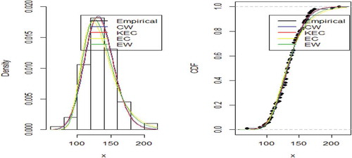
Compared to the competing models, the CW distribution with its four parameters provides a better fit for the datasets as it has the smallest value for all the goodness of fit measures used as shown in Table 5.

This is further confirmed by the plots of densities and cdfs of the empirical and fitted distributions as shown in Figures 4 and 5. From the fitted plot, it is observed that the CW provides a reasonable fit to the density.

Figure 5. Empirical and fitted density and cdf plots of data1

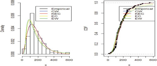
Figure 6. Empirical and fitted density and cdf plots of data2

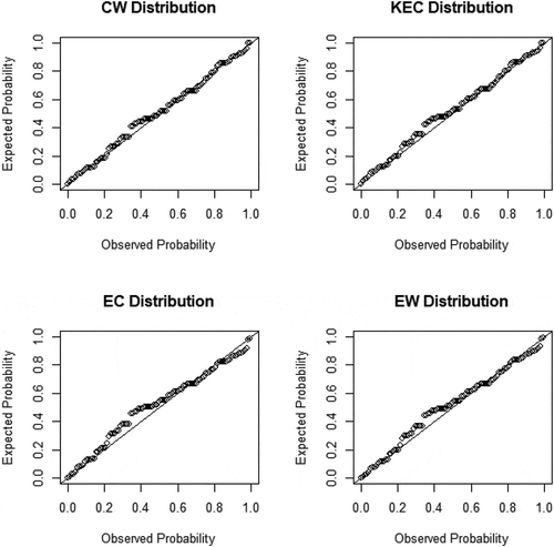
The P-P plots also indicates the CW distribution provides a better fit for both datasets in comparison with KEC, EC and EW distributions as shown in Figures 6 and 7.

Figure 7. P-P plots of fitted distributions for data1

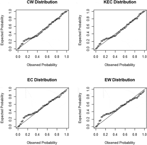
Figure 8. P-P plots of fitted distributions for data2

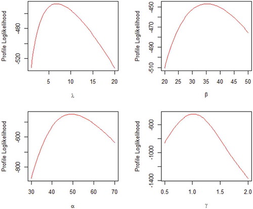
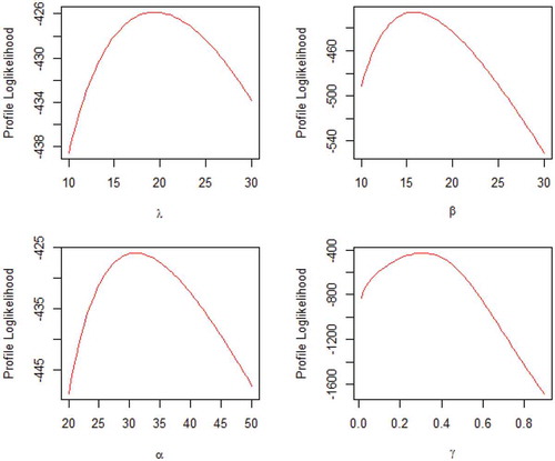
The profile likelihoods of the estimated parameters of the CW distribution for the datasets are shown in Figures 8 and 9. From the plots, it is observed that the estimated values for the parameters are the maxima.

Figure 9. Profile log-likelihood plot of CW parameters for data1

9. Conclusion

The focus of most researchers is geared towards developing new families of distributions for generalizing existing distributions to provide better fit for the modeling of life data. A new family of distribution called the CG family is developed and studied. Its statistical properties such as the quantile, moments, incomplete moments, generating function, entropies, stochastic ordering and order statistics are derived. Estimators for the parameters of the new family were developed using the method of maximum likelihood. A demonstration of the application of the special distribution developed from the family was carried out using two-real datasets. A comparison of the results with that of other existing distributions showed that the special distribution developed from the CG family provide a better parametric fit to these datasets.

Additional information

Funding

The authors received no direct funding for this research.

Notes on contributors

Lea Anzagra

Lea Anzagra is a doctoral candidate with the Department of Statistics, University for Development Studies, Ghana. Her research interest is in distribution theory, probability theory and survival analysis.

Solomon Sarpong

Solomon Sarpong is a Senior Lecturer with the Department of Statistics, University for Development Studies, Ghana. His research interest is in distribution theory and time series analysis.

Suleman Nasiru

Suleman Nasiru is a Senior Lecturer with the Department of Statistics, University for Development Studies, Ghana. His research interest is in distribution theory, quality control and time series analysis.

References

- Alzaatreh, A., Lee, C., & Famoye, F. (2013). A new method for generating families of continuous distributions. Metron, 71(1), 63–20. doi:10.1007/s40300-013-0007-y
- Birnbaum, Z. W., & Saunders, S. C. (1969). Estimation for a family of life distributions with applications to fatigue. Journal of Applied Probability, 6, 328–347. doi:10.2307/3212004
- Bjerkedal, T. (1960). Acquisition of resistance in guinea pies infected with different doses of virulent tubercle bacilli. American Journal of Hygeine, 72(1), 130–148.
- Bolker, B. (2014). Tools for general maximum likelihood estimation. R development core team.
- Burr, I. W. (1942). Cumulative frequency functions. Annals of Mathematical Statistics, 13, 215–232. doi:10.1214/aoms/1177731607
- Chaubey, Y. P., & Zhang, R. (2015). An extension of Chen’s family of survival distributions with bathtub shape or increasing hazard rate function. Communications in Statistics - Theory and Methods, 44(19), 4049–4064. doi:10.1080/03610926.2014.997357
- Chen, Z. (2000). A new two-parameter lifetime distribution with bathtub shape or increasing failure rate function. Statistics & Probability Letters, 49, 155–161. doi:10.1016/S0167-7152(00)00044-4
- Cordeiro, G. M., & de Castro, M. (2011). A new family of generalized distributions. Journal of Statistical Computation and Simulation, 81(7), 883–898. doi:10.1080/00949650903530745
- Hamedani, G. G., Yousof, H. M., Rasekhi, M., Alizadeh, M., & Najibi, S. M. (2018). Type I general exponential class of distributions. Pakistan Journal of Statistics and Operation Research, 14(1), 39–55. doi:10.18187/pjsor.v14i1.2193
- Khan, M. S., King, R., & Hudson, I. L. (2018). Kumaraswamy exponentiated Chen distribution for modelling lifetime data. Applied Mathematics and Information Sciences, 12(3), 617–623. doi:10.18576/amis/120317
- Kumaraswamy, P. (1980). Generalized probability density-function for double-bounded random-processes. Journal of Hydrology, 462, 79–88. doi:10.1016/0022-1694(80)90036-0
- Lee, C., Famoye, F., & Alzaatreh, A. Y. (2013). Methods for generating families of univariate continuous distributions in the recent decades. WIREs Computational Statistics, 5(3), 219–238. doi:10.1002/wics.1255
- Nasiru, S. (2018). Extended Odd Fréchet-G family of distributions. Journal of Probability and Statistics, 2018, 1–12. doi:10.1155/2018/2931326
- Nasiru, S., Mwita, P. N., & Ngesa, O. (2018). Exponentiated generalized power series family of distributions. Annals of Data Science, 6(3), 463–489. doi:10.1007/s40745-018-0170-3
- Rényi, A. (1961). On measures of entropy and information. Proceedings of the Fourth Berkeley Symposium on Mathematical Statistics and Probability, Contributions to the Theory of Statistics, 1, 547–561.
- Weibull, W. (1951). A statistical distribution function of wide applicability. Journal of Applied Mechanics, 18, 293–296.
- Xie, M., Tang, Y., & Goh, T. N. (2002). A modified Weibull extension with bathtub-shaped failure rate function. Reliability Engineering and System Safety, 76(3), 279–285. doi:10.1016/S0951-8320(02)00022-4
- Zubair, A. (2018). The Zubair-G family of distributions: Properties and applications. Annals of Data Science. doi:10.1007/s40745-018-0169-9