Effects of fractional and two-temperature parameters on stress distributions for an unbounded generalized thermoelastic medium with spherical cavity

Abstract

Effects of fractional and two-temperature parameters on the distribution of stresses of an unbounded isotropic thermoelastic medium with spherical cavity are studied in the context of the theory of two-temperature generalized thermoelasticity based on the Green-Naghdi model III using fractional order heat conduction equation. The surface of the cavity is considered to be free from traction and is subjected to a smooth and time-dependent-heating effect. A spherical polar coordinate system has been used to describe the problem and the resulting governing equations are solved in Laplace transform domain. Numerical Laplace transform inversion method has been then applied to get the stresses in time domain. The numerical estimates of the distributions of stresses are obtained and are presented graphically to study the effects of fractional and two-temperature parameters.

KEYWORDS AND PHRASES:

• Two-temperature generalized thermoelasticity
• Green-Naghdi model III
• time-fractional heat conduction
• spherical cavity

2010 Mathematics Subject Classification:

• 74F05

1. Introduction

Because of two major imperfections of the classical uncoupled theory of thermoelasticity, it became essential to make them modified. The first imperfection was the absence of elastic term in the heat conduction equation for which the theory failed to explain the phenomenon of heat generation due to elastic changes and conversely, elastic changes due to heat supply in thermoelastic solids. The parabolic nature of the heat conduction equation was the second imperfection recommending the infinite speed of propagation of thermal waves throughout the body (Peshkov, 1944). This means that, at any point of the body, thermal effect is realised instantaneously after the heat supply, which is not practically tenable. The elimination of the first imperfection was due to Biot (1955), who introduced an elastic term in the heat conduction equation. This theory is known as classical coupled theory of thermoelasticity. Still this theory was suffering from a second imperfection. To remove the second imperfection several developments and modifications were carried out by several researcher in different times. These modified theories are known as the generalized theory of thermoelasticity. The major contributions towards the formulation and development of generalized theory of thermoelasticity was due to Lord and Shulman (1967); Green and Lindsay (1972); Green and Naghdi (1991, 1992, 1993); Tzou (1995); Choudhuri (2007). For details one can refer to Ignaczak and Ostoja-Starzewski (2010) and Chandrasekharaiah (1986, 1998). It is to be noted that generalized theory of thermoelasticity can be applied to deal with practical problems where high heat fluxes appear for very short time-intervals, which generally occur in laser units, energy channels and nuclear reactors, etc. Many works have been carried out using these theories in the recent past, a few of which are mentioned hereunder. Abd-alla and Abbas (2002) have solved a magneto-thermoelastic problem for an infinitely long, perfectly conducting transversely isotropic cylinder using the theory of generalized thermoelasticity. Abbas and Youssef (2012) have established a generalized thermoelasticity model of temperature dependent materials and used it to solve a thermal shock problem of a generalized thermoelastic half-space by employing the finite element method. Abbas and Abo-Dahab (2014) have solved a thermal shock problem in generalized magneto-thermoelasticity for an infinitely long annular cylinder with variable thermal conductivity by using the Green-Lindsay model (Green & Lindsay, 1972).

The theory of heat conduction in elastically deformable bodies depends on two distinct temperatures; the conductive temperature ϕ and the thermodynamic temperature θ (Gurtin and Williams (1966); Gurtin and Williams (1967); Chen and Gurtin (1968); Chen, Gurtin and Williams (1968)). The first is due to thermal processes and the second is due to the mechanical processes inherent between the particles and the layers of the elastic material. The key element that sets the two-temperature thermoelasticity (2TT) apart from the classical theory of thermoelasticity (CTE) is the material parameter $a(\ge 0),$ called the temperature discrepancy (Chen, Gurtin & Williams, 1968; Chen & Gurtin, 1968). Specifically, if a = 0, then ϕ = θ and the field equations of the 2TT reduce to those of CTE.

Youssef has developed the theory of two-temperature generalized thermoelasticity based on the Lord-Shulman model (Youssef, 2006) and Green Naghdi model II (Youssef 2011). El-Karamany and Ezzat (2011) developed the theory of two-temperature generalized thermoelasticity for the Green Naghdi model III. They also established and proved the uniqueness and reciprocity theorems. Kumar, Prasad and Mukhopadhyay (2010) have studied the variational and the reciprocal principles in the context of two-temperature generalized thermoelasticity. Uniqueness and growth of solutions in two-temperature generalized thermoelasticity theories have been studied by Magañe and Quintanilla (2009). Abbas (2014a) has obtained general solution to the field equations of two-temperature Green-Naghdi theory for an unbounded medium with a spherical cavity by using an eigen-value approach. Abbas and Youssef (2013) have applied a finite element method to solve a two-dimensional problem for a thermoelastic half space under ramp-type heating using two-temperature Lord-Shulman theory (Youssef, 2006). Lotfy (2017) has studied photothermal waves in a semiconducting medium with hydrostatic initial stress using a two-temperature dual-phase-lag model (Mukhopadhyay, Prasad & Kumar, 2011).

In recent years, frequent applications of fractional calculus in many branches of applied sciences like solid mechanics, fluid mechanics, biology, physics and engineering etc. are observed. Due to the non-local property of the fractional operator, problems of applied sciences can be modelled better and more accurately using fractional calculus. Fractional calculus has been applied successfully to deal with problems related to dielectrics and semiconductors (Nigmatullin 1984a, 1984b; Scher & Montroll, 1975), porous (Koch & Brady, 1988) and random (Giona & Roman, 1992) media, porous glasses (Stapf, Kimmich & Seitter, 1995), polymer chains (Sokolov, Mai & Blumen, 1997), also to deal with problems related to biological systems (Ott, Bouchaud, Langevin & Urbach, 1990; Periasamy & Verkman, 1998). Details on the development and a survey of applications of the subject can be obtained in Podlubny (1999) and Ross (1977). Application of fractional calculus to a viscoelasticity problem was carried out by Caputo (1967) and Caputo and Mainardi (1971a, 1971b) and that to thermoelasticity was carried out by Povstenko (2004, 2011, 2015). Later, its application was extended to Generalized thermoelasticity by Sherief, El-Said and Abd El-Latief (2010), Youssef (2010) and Ezzat (2011a, 2011b). Ezzat, Elkaramany and Fayik (2012) have proposed a new model of thermoelasticity with three-phase-lag heat conduction in the context of a new consideration of time-fractional order Fourier’s law of heat conduction and also proved uniqueness and reciprocity theorems. They solved a one-dimensional problem for an elastic half-space in the presence of heat sources. Abbas (2014b) has solved a thermoelastic problem of functionally graded material using fractional order generalized thermoelasticity theory with one relaxation time. Mondal, Molla and Mallik (2017) have studied thermoelastic interactions in an infinite medium with a cylindrical cavity which is subjected to thermal and mechanical loading in the context of fractional order two-temperature generalized thermoelasticity under three phase lag heat transfer. Mallik, Molla and Mondal (2018) have solved a one-dimensional problem for an infinite solid with exponentially varying heat sources in the context of time-fractional two-temperature generalized thermoelasticity. Warbhe, Tripathi, Deshmukh and Verma (2018) have investigated the thermal deflection in a thin hollow circular disc subjected to time dependent heat flux in the context of fractional-order theory of thermoelasticity by a quasi-static approach. For more about the applications of fractional calculus one can refer to (Sun, Zhang, Baleanu, Chen & Chen, 2018).

The main object of this article is to study the effects of fractional and two-temperature parameters on the distribution of stresses of an unbounded isotropic thermoelastic medium with spherical cavity. The study has been carried out in the context of the theory of two-temperature generalized thermoelasticity based on the Green-Naghdi model III using a fractional order heat conduction equation. The surface of the cavity is considered to be free from traction and is subjected to a smooth and time-dependent-heating effect. A spherical polar coordinate system (r, ϑ, φ) has been used to describe the problem and the resulting governing equations are solved in Laplace transform domain. Laplace inversion of transformed stress components (radial stress and circumferential stress) has been carried out numerically by a method based on the Fourier series expansion technique (Honig & Hirdes, 1984). The numerical estimates of the distributions of stresses are obtained and are presented graphically to study the effects of fractional and two-temperature parameters.

2. Basic equations

The governing field equations for a homogeneous isotropic medium in the context of fractional order two-temperature generalized thermoelasticity theory based on the Green-Naghdi model III are as follows:

The strain displacement relation is (1) $$e_{\mathit{ij}}=\frac{1}{2}(u_{i,j}+u_{j,i}).$$(1)

The stress-strain temperature relation is (2) $${\tau }_{\mathit{ij}}=\lambda \Delta {\delta }_{\mathit{ij}}+2\mu e_{\mathit{ij}}-\gamma (\theta -{\theta }_0){\delta }_{\mathit{ij}},$$(2) where (3) $$\Delta =e_{\mathit{ii}}.$$(3)

The stress equation of motion in absence of body force is (4) $${\tau }_{\mathit{ij},j}=\rho \stackrel{..}{u_i}.$$(4)

The fractional heat conduction equation for two-temperature generalized thermoelasticity theory based on Green-Naghdi model III is (Akbarzadeh, Cui & Chen, 2017; Mallik, Molla and Mondal, 2018) (5) $$K{I}^{\alpha -1}{\dot{\varphi }}_{,\mathit{ii}}+K^{*}{I}^{\alpha -1}{\varphi }_{,\mathit{ii}}=\rho c_v\ddot{\theta }+\gamma {\theta }_0\text{div}\ddot{\overrightarrow{u}},$$(5) where the notation I^α refers to the Riemann-Liouville fractional integral, introduced as a natural generalization of the well-known n-fold repeated integral Iⁿf(t) written in a convolution-type form as follows (Mainardi & Gorenflo, 2000) (6) $$\begin{array}{c}{I}^{\alpha }f(r,t)=\frac{1}{\Gamma (\alpha )}{\int }_0^t{(t-\tau )}^{\alpha -1}f(r,\tau )d\tau ,\alpha >0,\\ =f(r,t),\alpha =0,\end{array}$$(6) Γ(α) being the Gamma function.

The parameter α indicates three different types of conductivities; 0 < α < 1 corresponds to weak conductivity, α = 1 corresponds to normal conductivity and 1 < α < 2 corresponds to strong conductivity in the medium (Youssef, 2010).

Here, λ and μ are Lamé constants, ρ is the density, c_v is specific heat at constant strain, $\gamma =(3\lambda +2\mu ){\alpha }_t,$ α_t being the coefficient of linear thermal expansion, θ₀ is the reference temperature, ϕ is conductive temperature, θ is the thermodynamic temperature, $\overrightarrow{u}$ is the displacement vector, K* is the material constant characteristic of the theory, K is the coefficient of thermal conductivity, comma in the subscript denotes derivative with respect to the next index (indices) and superscript dot denotes derivative with respect to time t.

Relation between the conductive temperature ϕ and thermodynamic temperature θ is (7) $$\varphi -\theta =a{\varphi }_{,\mathit{ii}},$$(7) where $a(\ge 0)$ is the two-temperature parameter (Chen, Gurtin & Williams, 1968; Chen & Gurtin, 1968).

3. Formulation of the problem

We consider an unbounded homogeneous isotropic thermoelastic medium with a spherical cavity of radius ‘ζ’. The centre of the cavity is considered as the origin of the spherical polar co-ordinate system (r, ϑ, φ), i.e. the medium occupies the region $\zeta \le r<\infty .$ Here we will consider spherical symmetric deformation of the medium so that displacement $\overrightarrow{u}=(u_r,u_{\vartheta },u_{\phi }),$ thermodynamic temperature θ and conductive temperature ϕ can be taken as follows: (8) $$u_r=u(r,t),u_{\vartheta }=u_{\phi }=0,\theta =\theta (r,t),\varphi =\varphi (r,t).$$(8)

Therefore we get (9) $$e_{\mathit{rr}}=\frac{\partial u}{\partial r},e_{\vartheta \vartheta }=e_{\phi \phi }=\frac{u}{r},e_{r\vartheta }=e_{r\phi }=e_{\vartheta \phi }=0,$$(9) and (10) $$\Delta =e_{\mathit{rr}}+e_{\vartheta \vartheta }+e_{\phi \phi }=\frac{\partial u}{\partial r}+\frac{2u}{r}.$$(10)

Hence the equation of motion (4) takes the form (11) $$\frac{\partial {\tau }_{\mathit{rr}}}{\partial r}+\frac{2}{r}({\tau }_{\mathit{rr}}-{\tau }_{\vartheta \vartheta })=\rho \frac{{\partial }^{2}u}{\partial t^2}.$$(11)

Equations (2)(2) $${\tau }_{\mathit{ij}}=\lambda \Delta {\delta }_{\mathit{ij}}+2\mu e_{\mathit{ij}}-\gamma (\theta -{\theta }_0){\delta }_{\mathit{ij}},$$(2) and (9)(9) $$e_{\mathit{rr}}=\frac{\partial u}{\partial r},e_{\vartheta \vartheta }=e_{\phi \phi }=\frac{u}{r},e_{r\vartheta }=e_{r\phi }=e_{\vartheta \phi }=0,$$(9) yield the non-zero stress components as (12) $${\tau }_{\mathit{rr}}=(\lambda +2\mu )\frac{\partial u}{\partial r}+2\lambda \frac{u}{r}-\gamma (\theta -{\theta }_0),$$(12) and (13) $${\tau }_{\vartheta \vartheta }={\tau }_{\phi \phi }=\lambda \frac{\partial u}{\partial r}+2(\lambda +\mu )\frac{u}{r}-\gamma (\theta -{\theta }_0).$$(13)

From Equations (5)(5) $$K{I}^{\alpha -1}{\dot{\varphi }}_{,\mathit{ii}}+K^{*}{I}^{\alpha -1}{\varphi }_{,\mathit{ii}}=\rho c_v\ddot{\theta }+\gamma {\theta }_0\text{div}\ddot{\overrightarrow{u}},$$(5) and (7)(7) $$\varphi -\theta =a{\varphi }_{,\mathit{ii}},$$(7) we get (14) $$\left[K{I}^{\alpha -1}\frac{\partial }{\partial t}+K^{*}{I}^{\alpha -1}+a\rho c_v\frac{{\partial }^2}{\partial t^2}\right]{\nabla }^2\varphi =\rho c_v\frac{{\partial }^2\varphi }{\partial t^2}+\gamma {\theta }_0\frac{{\partial }^2\Delta }{\partial t^2},$$(14) where ${\nabla }^2\equiv \frac{{\partial }^2}{\partial r^2}+\frac{2}{r}\frac{\partial }{\partial r}.$

Using Equations (12)(12) $${\tau }_{\mathit{rr}}=(\lambda +2\mu )\frac{\partial u}{\partial r}+2\lambda \frac{u}{r}-\gamma (\theta -{\theta }_0),$$(12) and (13)(13) $${\tau }_{\vartheta \vartheta }={\tau }_{\phi \phi }=\lambda \frac{\partial u}{\partial r}+2(\lambda +\mu )\frac{u}{r}-\gamma (\theta -{\theta }_0).$$(13) , the Equation (11)(11) $$\frac{\partial {\tau }_{\mathit{rr}}}{\partial r}+\frac{2}{r}({\tau }_{\mathit{rr}}-{\tau }_{\vartheta \vartheta })=\rho \frac{{\partial }^{2}u}{\partial t^2}.$$(11) reduces to (15) $$\left(\lambda +2\mu \right)\left[\frac{{\partial }^{2}u}{\partial t^2}+\frac{2}{r}\frac{\partial u}{\partial r}-\frac{2u}{r^2}\right]-\gamma \frac{\partial }{\partial r}\left[\varphi -a\left(\frac{{\partial }^2\varphi }{\partial r^2}+\frac{2}{r}\frac{\partial \varphi }{\partial r}\right)\right]=\rho \frac{{\partial }^{2}u}{\partial t^2}.$$(15)

We now introduce the following non-dimensional variables $$r\prime =c_0\eta r,u\prime =c_0\eta u,\zeta \prime =c_0\eta \zeta ,\theta \prime =\frac{\theta -{\theta }_0}{{\theta }_0},\varphi \prime =\frac{\varphi }{{\theta }_0},t\prime =c_0^2\eta t,$$ $$K^{*\prime }=\frac{K^{*}}{K{c}_0^2\eta },\tau {\prime }_{\mathit{ij}}=\frac{{\tau }_{\mathit{ij}}}{(\lambda +2\mu )},\Delta \prime =\Delta ,c_0^2=\frac{(\lambda +2\mu )}{\rho },\eta =\frac{\rho c_v}{K}.$$

Therefore we get Equations (7)(7) $$\varphi -\theta =a{\varphi }_{,\mathit{ii}},$$(7) and (12)–(15) in dimensionless form (for convenience we drop the primes) as follows (16) $$\varphi -\theta =\omega {\nabla }^2\varphi ,$$(16) (17) $${\tau }_{\mathit{rr}}=\frac{\partial u}{\partial r}+2{\lambda }_1\frac{u}{r}-a_1\theta ,$$(17) (18) $${\tau }_{\vartheta \vartheta }={\tau }_{\phi \phi }={\lambda }_1\frac{\partial u}{\partial r}+2({\lambda }_1+{\mu }_1)\frac{u}{r}-a_1\theta ,$$(18) (19) $$\left[I^{\alpha -1}\frac{\partial }{\partial t}+K^{*}{I}^{\alpha -1}+\omega \frac{{\partial }^2}{\partial t^2}\right]{\nabla }^2\varphi =\frac{{\partial }^2\varphi }{\partial t^2}+a_2\frac{{\partial }^2\Delta }{\partial t^2},$$(19) (20) $$\left[\frac{{\partial }^{2}u}{\partial r^2}+\frac{2}{r}\frac{\partial u}{\partial r}-\frac{2u}{r^2}\right]-a_1\left[\frac{\partial \varphi }{\partial r}-\omega \frac{\partial }{\partial r}\left(\frac{{\partial }^2\varphi }{\partial r^2}+\frac{2}{r}\frac{\partial \varphi }{\partial r}\right)\right]=\frac{{\partial }^{2}u}{\partial t^2},$$(20) where $a_1=\frac{\gamma {\theta }_0}{(\lambda +2\mu )},a_2=\frac{\gamma }{K\eta },{\lambda }_1=\frac{\lambda }{(\lambda +2\mu )},{\mu }_1=\frac{\mu }{(\lambda +2\mu )}$ and $\omega =a{c}_0^2{\eta }^2.$

4. Boundary conditions

We assume that the surface of the cavity (r = ζ) is stress free and is subjected to a thermal shock. The boundary conditions are therefore taken as follows (21) $${\tau }_{\mathit{rr}}{|}_{r=\zeta }=0,$$(21) (22) $$\varphi {|}_{r=\zeta }={\varphi }_{0}H\left(t\right),$$(22) where ϕ₀ is a constant and H(t) is the Heaviside unit step function.

5. Solution of the problem

For the solution of the problem we apply Laplace transform defined by (23) $$\overline{f}(r,p)={\int }_0^{\infty }{e}^{-\mathit{pt}}f(r,t)\mathit{dt},\mathit{Re}\left(p\right)>0.$$(23)

Therefore, taking Laplace transform on both sides of the Equations (16)–(22) we get (24) $$\overline{\varphi }-\overline{\theta }=\omega {\nabla }^2\overline{\varphi },$$(24) (25) $${\overline{\tau }}_{\mathit{rr}}=\frac{\partial \overline{u}}{\partial r}+2{\lambda }_1\frac{\overline{u}}{r}-a_1\overline{\theta },$$(25) (26) $${\overline{\tau }}_{\vartheta \vartheta }={\overline{\tau }}_{\phi \phi }={\lambda }_1\frac{\partial \overline{u}}{\partial r}+2({\lambda }_1+{\mu }_1)\frac{\overline{u}}{r}-a_1\overline{\theta },$$(26) (27) $$\left(p+K^{*}+\omega p^{\alpha +1}\right)\left(\frac{{\partial }^2}{\partial r^2}+\frac{2}{r}\frac{\partial }{\partial r}\right)\overline{\varphi }=p^{\alpha +1}(\overline{\varphi }+a_2\overline{\Delta }),$$(27) (28) $$\left[\frac{{\partial }^2\overline{u}}{\partial r^2}+\frac{2}{r}\frac{\partial \overline{u}}{\partial r}-\frac{2\overline{u}}{r^2}\right]-a_1\left[\frac{\partial \overline{\varphi }}{\partial r}-\omega \frac{\partial }{\partial r}\left(\frac{{\partial }^2\overline{\varphi }}{\partial r^2}+\frac{2}{r}\frac{\partial \overline{\varphi }}{\partial r}\right)\right]=p^2\overline{u},$$(28) (29) $${\overline{\tau }}_{\mathit{rr}}{|}_{r=\zeta }=0,$$(29) (30) $$\overline{\varphi }{|}_{r=\zeta }=\frac{{\varphi }_0}{p},$$(30) where $\overline{\Delta }=\frac{\partial \overline{u}}{\partial r}+\frac{2\overline{u}}{r}.$

Decoupling the Equations (27)(27) $$\left(p+K^{*}+\omega p^{\alpha +1}\right)\left(\frac{{\partial }^2}{\partial r^2}+\frac{2}{r}\frac{\partial }{\partial r}\right)\overline{\varphi }=p^{\alpha +1}(\overline{\varphi }+a_2\overline{\Delta }),$$(27) and (28)(28) $$\left[\frac{{\partial }^2\overline{u}}{\partial r^2}+\frac{2}{r}\frac{\partial \overline{u}}{\partial r}-\frac{2\overline{u}}{r^2}\right]-a_1\left[\frac{\partial \overline{\varphi }}{\partial r}-\omega \frac{\partial }{\partial r}\left(\frac{{\partial }^2\overline{\varphi }}{\partial r^2}+\frac{2}{r}\frac{\partial \overline{\varphi }}{\partial r}\right)\right]=p^2\overline{u},$$(28) we get (31) $$(D_{1}D-m_1^2)(D_{1}D-m_2^2)\overline{\varphi }=0,$$(31) (32) $$(D{D}_1-m_1^2)(D{D}_1-m_2^2)\overline{u}=0,$$(32) where $D\equiv \frac{\partial }{\partial r},D_1\equiv \frac{\partial }{\partial r}+\frac{2}{r}$ and $m_i^2,$ (i = 1, 2) are the roots of the equation (33) $$\left(p+K^{*}+\omega ϵp^{\alpha +1}\right)m^4-\left[p^2\left(p+K^{*}+\omega p^{\alpha +1}\right)+ϵp^{\alpha +1}\right]m^2+p^{\alpha +3}=0,$$(33) and we have used the notation, $ϵ=1+a_1{a}_2.$

The solution of the Equations (31)(31) $$(D_{1}D-m_1^2)(D_{1}D-m_2^2)\overline{\varphi }=0,$$(31) and (32)(32) $$(D{D}_1-m_1^2)(D{D}_1-m_2^2)\overline{u}=0,$$(32) with the conditions that they are bounded at infinity are respectively given by (34) $$\overline{\varphi }=\frac{1}{\sqrt{r}}\sum _{i=1}^2{g}_i{K}_{\frac{1}{2}}\left(m_{i}r\right),$$(34) (35) $$\overline{u}=\frac{1}{\sqrt{r}}\sum _{i=1}^2{h}_i{K}_{\frac{3}{2}}\left(m_{i}r\right),$$(35) where g_i and h_i, (i = 1, 2) are constants and $K_{\frac{1}{2}}(m_{i}r),K_{\frac{3}{2}}(m_{i}r)$ are the modified Bessel functions of the second kind of order $\frac{1}{2}$ and $\frac{3}{2}$ respectively.

The solution for $\overline{\theta }$ is now obtained from Equations (24)(24) $$\overline{\varphi }-\overline{\theta }=\omega {\nabla }^2\overline{\varphi },$$(24) and (34)(34) $$\overline{\varphi }=\frac{1}{\sqrt{r}}\sum _{i=1}^2{g}_i{K}_{\frac{1}{2}}\left(m_{i}r\right),$$(34) as (36) $$\overline{\theta }=\frac{1}{\sqrt{r}}\sum _{i=1}^2{g}_i\left[1-\omega m_i^2\right]K_{\frac{1}{2}}\left(m_{i}r\right).$$(36)

Using Equations (27), (34)(34) $$\overline{\varphi }=\frac{1}{\sqrt{r}}\sum _{i=1}^2{g}_i{K}_{\frac{1}{2}}\left(m_{i}r\right),$$(34) and (35)(35) $$\overline{u}=\frac{1}{\sqrt{r}}\sum _{i=1}^2{h}_i{K}_{\frac{3}{2}}\left(m_{i}r\right),$$(35) we get the relations between the constants g_i and h_i as follows: (37) $$h_i=l_i{g}_i,\text{where}{l}_i=\frac{p^{\alpha +1}-(p+K^{*}+\omega p^{\alpha +3})m_i^2}{a_2{p}^{\alpha +1}{m}_i},i=1,2.$$(37)

Thus, from Equations (25)(25) $${\overline{\tau }}_{\mathit{rr}}=\frac{\partial \overline{u}}{\partial r}+2{\lambda }_1\frac{\overline{u}}{r}-a_1\overline{\theta },$$(25) and (26)(26) $${\overline{\tau }}_{\vartheta \vartheta }={\overline{\tau }}_{\phi \phi }={\lambda }_1\frac{\partial \overline{u}}{\partial r}+2({\lambda }_1+{\mu }_1)\frac{\overline{u}}{r}-a_1\overline{\theta },$$(26) we get the solutions for ${\overline{\tau }}_{\mathit{rr}},{\overline{\tau }}_{\vartheta \vartheta }$ and ${\overline{\tau }}_{\phi \phi }$ as (38) $${\overline{\tau }}_{\mathit{rr}}=\sum _{i=1}^2{g}_i{S}_i^r,$$(38) (39) $${\overline{\tau }}_{\phi \phi }={\overline{\tau }}_{\vartheta \vartheta }=\sum _{i=1}^2{g}_i{S}_i^{\phi },$$(39) where (40) $$S_i^r=\frac{1}{\sqrt{r}}[l_i\{-m_i{K}_{\frac{1}{2}}\left(m_{i}r\right)+\frac{2}{r}({\lambda }_1-1)K_{\frac{3}{2}}\left(m_{i}r\right)\}-a_1(1-\omega m_i^2\left)K_{\frac{1}{2}}\right(m_{i}r)], i=1,2,$$(40) and (41) $$S_i^{\phi }=\frac{1}{\sqrt{r}}[l_i\{-{\lambda }_1{m}_i{K}_{\frac{1}{2}}\left(m_{i}r\right)+\frac{2{\mu }_1}{r}{K}_{\frac{3}{2}}\left(m_{i}r\right)\}-a_1(1-\omega m_i^2\left)K_{\frac{1}{2}}\right(m_{i}r)], i=1,2.$$(41)

Using (29) and (30) we obtain the constants g₁ and g₂ as follows (42) $$g_1=\frac{-{\varphi }_0\sqrt{\zeta }{S}_2^{\zeta }}{p\left[S_1^{\zeta }{K}_{\frac{1}{2}}\right(m_2\zeta )-S_2^{\zeta }{K}_{\frac{1}{2}}(m_1\zeta \left)\right]},$$(42) (43) $$g_2=\frac{{\varphi }_0\sqrt{\zeta }{S}_1^{\zeta }}{p\left[S_1^{\zeta }{K}_{\frac{1}{2}}\right(m_2\zeta )-S_2^{\zeta }{K}_{\frac{1}{2}}(m_1\zeta \left)\right]},$$(43) where (44) $$S_i^{\zeta }=\frac{1}{\sqrt{\zeta }}[l_i\{-m_i{K}_{\frac{1}{2}}(m_i\zeta )+\frac{2}{\zeta }({\lambda }_1-1)K_{\frac{3}{2}}(m_i\zeta )\}-a_1(1-\omega m_i^2\left)K_{\frac{1}{2}}\right(m_i\zeta )],i=1,2.$$(44)

6. Numerical inversion of Laplace transform

It is difficult to find the analytical inverse of Laplace transform of the complicated solutions for the stress components in the Laplace transform domain. So we have to resort to numerical computations. We now outline the numerical procedure to solve the problem. Let $\overline{f}(r,p)$ be the Laplace transform of a function f(r, t). Then, the inversion formula for Laplace transform can be written as (45) $$f(r,t)=\frac{1}{2\pi i}{\int }_{d-i\infty }^{d+i\infty }{e}^{\mathit{pt}}\overline{f}(r,p)\mathit{dp},$$(45) where d is an arbitrary real number greater than real parts of all the singularities of $\overline{f}(r,p).$ Taking $p=d+\mathit{iw},$ the preceding integral takes the form (46) $$f(r,t)=\frac{e^{\mathit{dt}}}{2\pi }{\int }_{-\infty }^{+\infty }{e}^{\mathit{itw}}f(r,d+\mathit{iw})\mathit{dw}.$$(46)

Expanding the function $h(r,t)=e^{-\mathit{dt}}f(r,t)$ in a Fourier series in the interval [0, 2 T], we obtain the approximate formula (Honig & Hirdes, 1984) (47) $$f(r,t)=f_{\infty }(r,t)+E_D,$$(47) where (48) $$f_{\infty }(r,t)=\frac{1}{2}{c}_0+\sum _{k=1}^{\infty }{c}_k, \text{for} 0\le t\le 2T,$$(48) and (49) $$c_k=\frac{e^{\mathit{dt}}}{T}\left[e^{\frac{\mathit{ik}\pi t}{T}}\overline{f}(r,d+\frac{\mathit{ik}\pi t}{T})\right].$$(49)

The discretization error E_D can be made arbitrary small by choosing d large enough (Honig & Hirdes, 1984). Since the infinite series in (48) can be summed up to a finite number N of terms, the approximate value of f(r, t) becomes (50) $$f_N(r,t)=\frac{1}{2}{c}_0+\sum _{k=1}^N{c}_k,\text{for}0\le t\le 2T.$$(50)

Using the preceding formula to evaluate f(r, t), we introduce a truncation error E_T that must be added to the discretization error to produce total approximation error.

Two methods are used to reduce the total error. First, the Korrektur method is used to reduce the discretization error. Next, the ε-algorithm is used to accelerate the convergence (Honig & Hirdes, 1984)

The Korrektur method uses the following formula to evaluate the function f(r, t): (51) $$f(r,t)=f_{\infty }(r,t)-e^{-2dT}{f}_{\infty }(r,2T+t)+E_D^{\prime },$$(51) where the discretization error $\left|E_D^{\prime }\right|\ll \left|E_D\right|$. Thus, the approximate value of f(r, t) becomes (52) $$f_{\mathit{NK}}(r,t)=f_N(r,t)-e^{-2dT}{f}_{N^{\prime }}(r,2T+t),$$(52) where $N^{\prime }$ is an integer such that $N^{\prime }<N.$

We shall now describe the ε-algorithm that is used to accelerate the convergence of the series in Equation (46)(46) $$f(r,t)=\frac{e^{\mathit{dt}}}{2\pi }{\int }_{-\infty }^{+\infty }{e}^{\mathit{itw}}f(r,d+\mathit{iw})\mathit{dw}.$$(46) . Let $N=2q+1,$ where q is a natural number and let $s_m={\sum }_{k=1}^m{c}_k$ be the sequence of partial sums of series in (48). We define the ε-sequence by $${\epsilon }_{0,m}=0,{\epsilon }_{1,m}=s_m$$ and $${\epsilon }_{p+1,m}={\epsilon }_{p-1,m+1}+\frac{1}{{\epsilon }_{p,m+1}-{\epsilon }_{p,m}},p=1,2,3\dots ..$$

It can be shown (Honig & Hirdes, 1984) that the sequence $${\epsilon }_{1,1},{\epsilon }_{3,1},{\epsilon }_{5,1},\dots ..{\epsilon }_{N,1},$$ converges to $f(r,t)+E_D-\frac{c_0}{2}$ faster than the sequence of partial sums s_m, $m=1,2,3,\dots ...$

The actual procedure used to invert the Laplace transform consists of using Equation (51)(51) $$f(r,t)=f_{\infty }(r,t)-e^{-2dT}{f}_{\infty }(r,2T+t)+E_D^{\prime },$$(51) together with the ε-algorithm. The values of d and T are chosen according to the criterion outlined in (Honig & Hirdes, 1984).

7. Numerical results and discussion

To get the solutions for the radial stress (τ_rr) and the circumferential stress (${\tau }_{\phi \phi }$) in the space-time domain, we have to apply numerical inversion of the Laplace transform. This has been done numerically using a method based on the Fourier series expansion technique as mentioned above (Honig & Hirdes, 1984). The numerical code has been prepared using the Fortran programming language. For the purpose of illustration, we have used the copper like material for which the material constants are given below (Youssef, 2010). $$\begin{array}{c}K=386N/\mathit{Ks},{\alpha }_t=1.78\times {10}^{-5}{K}^{-1},\\ \lambda =7.76\times {10}^{10}N/m^2,\mu =3.86\times {10}^{10}N/m^2\\ \rho =8,954kg/m^3,{\theta }_0=293K,ϵ=1.0168,K^{*}=7.\end{array}$$

The computations were carried out for t = 0.4. The radial stress (τ_rr) and the circumferential stress (${\tau }_{\phi \phi }$) are represented graphically against different values of r for weak conductivity (α = 0.5), normal conductivity (α = 1.0) and strong conductivity (α = 1.2) for both one-temperature (ω = 0.0) and two-temperature (ω = 0.1, 0.2) theories, respectively.

Figures 1a and 1b are drawn to study the effects fractional parameter α on radial stress (τ_rr) and circumferential stress (${\tau }_{\phi \phi }$) in one-temperature theory (ω = 0.0) whereas the Figures 2a and 2b are drawn to study the effects fractional parameter α on radial stress (τ_rr) and circumferential stress (${\tau }_{\phi \phi }$) in two-temperature theory (ω = 0.1). The Figures 3a, 3b; 4a, 4b and 5a, 5b are drawn to study the effects two-temperature parameter ω on radial stress (τ_rr) and circumferential stress (${\tau }_{\phi \phi }$) in weak conductivity (α = 0.5), normal conductivity (α = 1.0) and strong conductivity (α = 1.2) respectively.

Figure 1. (a) Variation of radial stress ${\tau }_{\mathit{rr}}$ with r for $\omega$ = 0.0. (b) Variation of circumferential stress ${\tau }_{\phi \phi }$ with r for $\omega$ = 0.0.

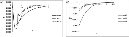
Figure 2. (a) Variation of radial stress ${\tau }_{\mathit{rr}}$ with r for $\omega$ = 0.1. (b) Variation of circumferential stress ${\tau }_{\phi \phi }$ with r for $\omega$ =0.1.

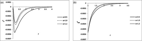
Figure 3. (a) Variation of radial stress ${\tau }_{\mathit{rr}}$ with r for $\alpha$ = 0.5. (b) Variation of circumferential stress ${\tau }_{\phi \phi }$ with r for $\alpha$ = 0.5.

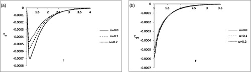
Figure 4. (a) Variation of radial stress ${\tau }_{\mathit{rr}}$ with r for $\alpha$ = 1.0. (b) Variation of circumferential stress ${\tau }_{\phi \phi }$ with r for $\alpha$ = 1.0.

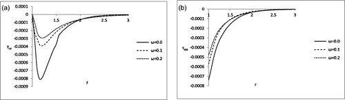
Figure 5. (a) Variation of radial stress ${\tau }_{\mathit{rr}}$ with r for $\alpha$ = 1.2. (b) Variation of circumferential stress ${\tau }_{\phi \phi }$ with r for $\alpha$ =1.2.

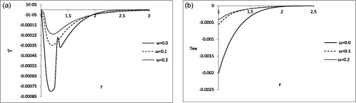
Observing the Figure 1a we see that at the boundary of the cavity, the radial stress (τ_rr) vanishes in all types of conductivities satisfying our assumed stress free boundary condition. The maximum magnitude of the radial stress (τ_rr) is attained for strong conductivity (α = 1.2) and the radial stress for strong conductivity tends to vanish for smaller values of r compared to normal and weak conductivities.

Figure 1b shows that the circumferential stress (${\tau }_{\phi \phi }$) is compressive in nature in all types of conductivities and the maximum magnitude of the circumferential stress (${\tau }_{\phi \phi }$) in all types of conductivities is attained at the boundary of the cavity. The effects of the fractional parameter α is prominent in the region $1.0\le r\le 1.75$ (approx.) and afterwards no significant effect is found.

From Figures 2a and 2b it is observed that the magnitudes of the radial stress (τ_rr) and the circumferential stress (${\tau }_{\phi \phi }$) is largest for weak conductivity (α = 0.5) and smallest for strong conductivity (α = 1.2). For strong conductivity, both stresses tend to vanish for smaller values of r compared to normal and weak conductivities.

Figure 3a exhibits that almost there is no effect of two-temperature parameter ω upon radial stress (τ_rr) distribution at the vicinity of the boundary of the spherical cavity. But a slight effect of two-temperature parameter ω upon circumferential stress $({\tau }_{\phi \phi })$ distribution is revealed near to the boundary of the spherical cavity as exhibited in Figure 3b.

From Figures 4a and 4b we observe that the effects of two-temperature parameter ω on radial stress (τ_rr) distribution and circumferential stress $({\tau }_{\phi \phi })$ distribution are more prominent compared to the Figures 3a and 3b.

Figures 5a and 5b show that the effects of two-temperature parameter ω on radial stress (τ_rr) distribution and circumferential stress $({\tau }_{\phi \phi })$ distribution at the vicinity of the boundary of the spherical cavity is very prominent, which was not the case in Figures 3a and 3b, respectively. In the two Figures 5a and 5b the effects of two-temperature parameter ω is also more prominent compared to the Figures 4a and 4b, respectively.

8. Conclusions

The problem of investigating the radial stress (τ_rr) and circumferential stress $({\tau }_{\phi \phi })$ in an infinite, homogeneous, isotropic medium with spherical cavity is studied in the light of two-temperature generalized thermoelasticity theory based on Green-Naghdi model III in the context of time fractional heat conduction equation. A spherical polar coordinate system has been used to describe the problem and the solution is obtained in the Laplace transform domain. Numerical inversion of Laplace transform is done by using the Fourier series expansion technique (Honig & Hirdes, 1984). The analysis of the results allows us to make the following conclusions:

1. Stress components vanish after a certain distance in conformity with the generalized theory of thermoelasticity.

2. Significant effects of two-temperature parameter ω on the distributions of stresses for different types of conductivities and the effect of fractional parameter α on the distributions of stresses for both one-temperature and two-temperature theories are observed.

3. For both one-temperature and two-temperature theories, a tendency of vanishing of stress components starts at a smaller distance from the surface of the spherical cavity, for larger value of fractional parameter α (Figures 1a, 1b, 2a, 2b).

4. Effects of the two-temperature parameter ω on the distributions of stresses become more and more prominent with the increase of the values of fractional parameter α (Figures 3a, 3b, 4a, 4b, 5a, 5b).

Acknowledgements

The authors would like to express their sincere thanks to the referees for helpful comments and suggestions for the improvement of this paper.

Disclosure statement

No potential conflict of interest was reported by the author(s).

References

- Abbas, I. A. (2014a). A GN model based upon two-temperature generalized thermoelastic theory in an unbounded medium with a spherical cavity. Applied Mathematics and Computation, 245(C), 108–115. doi:10.1016/j.amc.2014.07.059
- Abbas, I. A. (2014b). A problem on functional graded material under fractional order theory of thermoelasticity. Theoretical and Applied Fracture Mechanics, 74, 18–22. doi:10.1016/j.tafmec.2014.05.005
- Abbas, I. A., & Abo-Dahab, S. M. (2014). On the numerical solution of thermal shock problem for generalized magneto-thermoelasticity for an infinitely long annular cylinder with variable thermal conductivity. Journal of Computational and Theoretical Nanoscience, 11(3), 607–618. doi:10.1166/jctn.2014.3402
- Abbas, I. A., & Youssef, H. M. (2012). A nonlinear generalized thermoelasticity model of temperature-dependent materials using finite element method. International Journal of Thermophysics, 33(7), 1302–1313. doi:10.1007/s10765-012-1272-3
- Abbas, I. A., & Youssef, H. M. (2013). Two-temperature generalized thermoelasticity under ramp-type heating by finite element method. Meccanica, 48(2), 331–339. doi:10.1007/s11012-012-9604-8
- Abd-Alla, N. A., & Abbas, I. A. (2002). A problem of generalized magnetothermoelasticity for an infinitely long, perfectly conducting cylinder. Journal of Thermal Stresses, 25(11), 1009–1025. doi:10.1080/01495730290074612
- Akbarzadeh, A. H., Cui, Y., & Chen, Z. T. (2017). Thermal wave: From nonlocal continuum to molecular dynamics. RSC Advances, 7(22), 13623–13636. doi:10.1039/C6RA28831F
- Biot, M. (1955). Variational principle in irreversible thermodynamics with application to viscoelasticity. Physical Review, 97(6), 1463–1469. doi:10.1103/PhysRev.97.1463
- Caputo, M. (1967). Linear model of dissipation whose Q is always frequency independent. Geophysical Journal of the Royal Astronomical Society, 13(5), 529–539. doi:10.1111/j.1365-246X.1967.tb02303.x
- Caputo, M., & Mainardi, F. (1971a). A new dissipation model based on memory mechanism. Pure and Applied Geophysics Pageoph, 91(1), 134–147. doi:10.1007/BF00879562
- Caputo, M., & Mainardi, F. (1971b). Linear model of dissipation in an elastic solids. La Rivista Del Nuovo Cimento, 1(2), 161–198. doi:10.1007/BF02820620
- Chandrasekharaiah, D. S. (1986). Thermoelasticity with second sound: A review. Applied Mechanics Reviews, 39(3), 355–376. doi:10.1115/1.3143705
- Chandrasekharaiah, D. S. (1998). Hyperbolic thermoelasticity, a review of recent literature. Applied Mechanics Reviews, 51(12), 705–729. doi:10.1115/1.3098984
- Chen, P. J., & Gurtin, M. E. (1968). On a theory of heat conduction involving two temperatures. Zeitschrift Für Angewandte Mathematik Und Physik Zamp, 19(4), 614–627. doi:10.1007/BF01594969
- Chen, P. J., Gurtin, M. E., & Williams, W. O. (1968). A note on non-simple heat conduction. Zeitschrift Für Angewandte Mathematik Und Physik Zamp, 19(6), 969–970. doi:10.1007/BF01602278
- Choudhuri, S. K. R. (2007). On a thermoelastic three-phase-lag model. Journal of Thermal Stresses, 30(3), 231–238. doi:10.1080/01495730601130919
- El-Karamany, A. S., & Ezzat, M. A. (2011). On the two-temperature Green-Naghdi thermoelasticity theories. Journal of Thermal Stresses, 34(12), 1207–1226. doi:10.1080/01495739.2011.608313
- Ezzat, M. A. (2011a). Theory of fractional order in generalized thermoelectric MHD. Applied Mathematical Modelling, 35(10), 4965–4978. doi:10.1016/j.apm.2011.04.004
- Ezzat, M. A. (2011b). Magneto-thermoelasticity with thermoelectric properties and fractional derivative heat transfer. Physica B: Condensed Matter, 406(1), 30–35. doi:10.1016/j.physb.2010.10.005
- Ezzat, M. A., El Karamany, A. S., & Fayik, M. A. (2012). Fractional order theory in thermoelastic solid with three-phase lag heat transfer. Archive of Applied Mechanics, 82(4), 557–572. doi:10.1007/s00419-011-0572-6
- Giona, M., & Roman, H. E. (1992). Fractional diffusion equation for transport phenomena in random media. Physica A, 185(1–4), 87–97. doi:10.1016/0378-4371(92)90441-R
- Green, A. E., & Lindsay, K. A. (1972). Thermoelasticity. Journal of Elasticity, 2(1), 1–7. doi:10.1007/BF00045689
- Green, A. E., & Naghdi, P. M. (1991). A re-examination of the basic postulates of thermomechanics. Proceedings of the Royal Society A, 432(1885), 171–194. doi:10.1098/rspa.1991.0012
- Green, A. E., & Naghdi, P. M. (1992). On undamped heat waves in an elastic solid. Journal of Thermal Stresses, 15, 252–264.
- Green, A. E., & Naghdi, P. M. (1993). Thermoelasticity without energy dissipation. Journal of Elasticity, 31(3), 189–208. doi:10.1007/BF00044969
- Gurtin, M. E., & Williams, W. O. (1966). On the Clausius-Duhem inequality. Zeitschrift Für Angewandte Mathematik Und Physik Zamp, 17(5), 626–633. doi:10.1007/BF01597243
- Gurtin, M. E., & Williams, W. O. (1967). An axiomatic foundation for continuum thermodynamics. Archive for Rational Mechanics and Analysis, 26(2), 83–117. doi:10.1007/BF00285676
- Honig, G., & Hirdes, U. (1984). A method for the numerical inversion of the Laplace transform. Journal of Computational and Applied Mathematics, 10(1), 113–132. doi:10.1016/0377-0427(84)90075-X
- Ignaczak, J., & Ostoja-Starzewski, M. (2010). Thermoelasticity with finite wave speeds. New York: Oxford University Press Inc.
- Koch, D. L., & Brady, J. F. (1988). Anomalous diffusion in heterogeneous porous media. Physics of Fluids, 31(5), 965–973. doi:10.1063/1.866716
- Kumar, R., Prasad, R., & Mukhopadhyay, S. (2010). Variational and reciprocal principles in two-temperature generalized thermoelasticity. Journal of Thermal Stresses, 33(3), 161–171. doi:10.1080/01495730903454678
- Lord, H., & Shulman, Y. (1967). A generalized dynamical theory of thermoelasticity. Journal of the Mechanics and Physics of Solids, 15(5), 299–309. doi:10.1016/0022-5096(67)90024-5
- Lotfy, K. (2017). Photothermal waves for two temperature with semiconducting medium under using a dual-phase-lag model and hydrostatic initial stress. Waves in Random and Complex Media, 27(3), 482–501. doi:10.1080/17455030.2016.1267416
- Magañe, A., & Quintanilla, R. (2009). Uniqueness and growth of solutions in two-temperature generalized thermoelastic theories. Mathematics and Mechanics of Solids, 14, 622–634. doi:10.1177/1081286507087653
- Mainardi, F., & Gorenflo, R. (2000). On Mittag-Lettler-type function in fractional evolution processes. Mathematics and Mechanics of Solids, 118, 283–299. doi:10.1016/S0377-0427(00)00294-6
- Mallik, S. H., Molla, M. A. K., & Mondal, N. (2018). Time-fractional two-temperature generalized thermoelasticity with energy dissipation for an infinite solid with varying heat sources. Bulletin of the Calcutta Mathematical Society, 110(5), 419–440.
- Mondal, N., Molla, M. A. K., & Mallik, S. H. (2017). Fractional order two temperature generalized thermoelasticity of an infinite medium with cylindrical cavity under three phase lag heat transfer. Indian Journal of Theoretical Physics, 65(3-4), 187–203.
- Mukhopadhyay, S., Prasad, R., & Kumar, R. (2011). On the theory of two-temperature thermoelasticity with two phase-lags. Journal of Thermal Stresses, 34(4), 352–365. doi:10.1080/01495739.2010.550815
- Nigmatullin, R. R. (1984a). On the theory of relaxation for systems with “Remnant” memory. Physica Status Solidi (b)), 124(1), 389–393. doi:10.1002/pssb.2221240142
- Nigmatullin, R. R. (1984b). To the theoretical explanation of the “Universal Response”. Physica Status Solidi (b)), 123(2), 739–745. doi:10.1002/pssb.2221230241
- Ott, A., Bouchaud, J. P., Langevin, D., & Urbach, W. (1990). Anomalous diffusion in “Living Polymers”: A Genuine Levy Flights? Physical Review Letters, 65(17), 2201–2204. doi:10.1103/PhysRevLett.65.2201
- Periasamy, N., & Verkman, A. S. (1998). Analysis of fluorophore diffusion by continuous distributions of diffusion coefficients: Application to photobleaching measurements of multicomponent and anomalous diffusion. Journal of Biophysics, 75(1), 557–567. doi:10.1016/S0006-3495(98)77545-9
- Peshkov, V. (1944). Second sound in helium II. Journal of Physics, 8, 381–382.
- Podlubny, I. (1999). Fractional differential equations. New York: Academic press.
- Povstenko, Y. Z. (2004). Fractional heat conduction equation and associated thermal stress. Journal of Thermal Stresses, 28(1), 83–102. doi:10.1080/014957390523741
- Povstenko, Y. Z. (2011). Fractional Catteneo-type equations and generalized thermoelasticity. Journal of Thermal Stresses, 34, 94–114.
- Povstenko, Y. Z. (2015). Fractional thermoelasticity. Switzerland: Springer International Publishing.
- Ross, B. (1977). The development of fractional calculus 1695-1900. Historia Mathematica, 4(1), 75–89. doi:10.1016/0315-0860(77)90039-8
- Scher, H., & Montroll, E. W. (1975). Anomalous transit-time dispersion in amorphous solid. Physical Review B, 12(6), 2455–2477. doi:10.1103/PhysRevB.12.2455
- Sherief, H. H., El-Sayed, A. M. A., & Abd El-Latief, A. M. (2010). Fractional order theory of thermoelasticity. International Journal of Solids and Structures, 47(2), 269–275. doi:10.1016/j.ijsolstr.2009.09.034
- Sokolov, I. M., Mai, J., & Blumen, A. (1997). Paradoxal diffusion in chemical space for nearest-neighbor walks over polymer chains. Physical Review Letters, 79(5), 857–860. doi:10.1103/PhysRevLett.79.857
- Stapf, S., Kimmich, R., & Seitter, R. O. (1995). Proton and deuteron field-cycling NMR relaxometry of liquids in porous glasses: Evidence for Lévy-walk statistics. Physical Review Letters, 75(15), 2855–2858. doi:10.1103/PhysRevLett.75.2855
- Sun, H. G., Zhang, Y., Baleanu, D., Chen, W., & Chen, Y. Q. (2018). A new collection of real world applications of fractional calculus in science and engineering. Communications in Nonlinear Science and Numerical Simulations, 64, 213–231. doi:10.1016/j.cnsns.2018.04.019
- Tzou, D. Y. (1995). A unified field approach for heat conduction from macro-to micro-scales. Journal of Heat Transfer, 117(1), 8–17. doi:10.1115/1.2822329
- Warbhe, S. D., Tripathi, J. J., Deshmukh, K. C., & Verma, J. (2018). Fractional heat conduction in a thin hollow circular disk and associated thermal deflection. Journal of Thermal Stresses, 41(2), 262–270. doi:10.1080/01495739.2017.1393645
- Youssef, H. M. (2006). Theory of two-temperature generalized thermoelasticity. IMA Journal of Applied Mathematics, 71, 1–8.
- Youssef, H. M. (2010). Theory of fractional order generalized thermoelasticity. ASME Journal of Heat Transfer, 132, 1–7.
- Youssef, H. M. (2011). Theory of two-temperature thermoelasticity without energy dissipation. Journal of Thermal Stresses, 34(2), 138–146. doi:10.1080/01495739.2010.511941