Thermomechanical interactions in transversely isotropic magneto-thermoelastic medium with fractional order generalized heat transfer and hall current

Abstract

This investigation is focused on the study of thermomechanical interactions in homogeneous transversely isotropic magneto thermoelastic medium with fractional order heat transfer and hall current. As an application, the bounding surface is subjected to normal force with weak, normal and strong conductivity. Laplace and Fourier transform is used for solving field equations. The analytical expressions of temperature, displacement components, stress components, and current density components are computed in the transformed domain. The effects of hall current and fractional order parameters by varying different values are represented graphically. Some specific cases are also figured out from the current research.

Keywords:

• Laplace and Fourier transform
• thermoelastic
• hall current
• transversely isotropic
• fractional order heat transfer

1. Introduction

Classical Theory (CT) of elasticity is concerned with the systematic study of the stress and strain distribution that develops in an elastic body due to the application of forces or variations in temperature. Temperature changes result in thermal effects on materials like thermal stress, strain, and deformation. When external force or loads is applied to a material body, it generates mechanical waves. For example, if a sudden heat is applied in a solid body, it will produce a mechanical wave through thermal expansion. It was observed that the interaction s between the thermal and mechanical fields occurred through the Lorentz forces, Ohm’s law and the electric field created by the velocity of a material particle, moving in a magnetic field. Thermal dependency is the primary contrast of thermoelasticity concerning to the classical theory of thermomechanics. The study of the interaction between mechanical and thermal fields in the anisotropic media particularly transversely isotropic is one of the most extensive and productive areas of continuum dynamics. When the magnetic field is very strong, the influence of Hall current cannot be ignored. However, due to a greater number of elastic and thermal coefficients involved, there are not so many solutions available as there are for isotropic media.

Abel firstly used the fractional derivatives in applied fractional calculus for finding the solution of an integral equation of the tautochrone problem. The complete theory of fractional derivatives and integrals was established in the middle of the 19th century by Caputo (1967) and proved with experimental results of fractional derivatives for viscoelastic materials and proven the relation between fractional order derivatives and the theory of linear viscoelasticity. Ezzat, El-Karamany, and Fayik (2012) studied the linear thermoelasticity theory using the Fourier law of heat conduction with time-fractional order and three-phase lag. Elsafty (2015) studied the problem of thermoelastic half-space by using the fractional order theory of thermoelasticity, in which the bounding surface is subjected to a time-dependent thermal shock. Bachher and Sarkar (2016) studied the Caputo time-fractional derivative for the magneto-thermoelastic response of a homogeneous isotropic 2D elastic half-space solid with rotation. Sheoran and Kundu (2016) gave a review and future prospects of fractional order generalized thermoelasticity theory. Kumar, Sharma, and Lata (2017) investigated the Rayleigh waves in a homogeneous transversely isotropic magneto-thermoelastic in the presence of two temperature, hall current, and rotation. Moreno-Navarro, Ibrahimbegovic, and Pérez-Aparicio (2018) proposed a fully coupled thermodynamic oriented transient finite element formulation for magnetic, electric, mechanic and thermal field interactions.

Youssef and Abbas (2014) considered fractional order thermal conductivity as a linear function of temperature in the perspective of fractional order generalized thermoelasticity. Tripathi, Deshmukh, and Verma (2017) studied the generalized thermoelasticity fractional order thermoelastic response due to a heat source that varies periodically with time with one relaxation time. Abbas (2018) studied the effect of fractional order 2-D GN-III model due to thermal shock for weak, normal and strong conductivity. Kumar et al. (2017) studied the thermomechanical interactions and effect of hall current and magnetic field in a homogeneous transversely isotropic thermoelastic medium with rotation and two temperatures using GN-II and III theories. Ezzat, El-Karamany, and El-Bary (2018) developed a unified mathematical fractional model of two-temperature phase-lag GN thermoelasticity theories. Ezzat, El-Karamany, and Ezzat (2012), Ezzat and El-Bary (2017) presented a new mathematical model of 2T electro-thermo viscoelasticity theory in the context of heat conduction and provided applications of this model to different problems like concrete problems, a thermal shock problem and a problem for a half-space exposed to ramp-type heating respectively. Despite of this several researchers worked on different theory of thermoelasticity as Mahmoud, Abd-Alla, and El-Sheikh (2011), Mahmoud, Marin, & Al-Basyouni (2015), Mahmoud (2012), Abbas and Youssef (2009, 2013), Kumar, Sharma, and Lata (2016a, 2016b), Lata (2017), Marin, Baleanu, and Vlase (2017, 2018) and Lata and Kaur (2018, 2019a, 2019b), Kaur and Lata (2019a, 2019b, 2019c).

A lot of research had been carried out by the various researches in different fields of thermoelasticity Inspite of these, not much work has been carried out in the study of the effect of hall current due to fractional order three phase lag heat transfer. In this paper, we have attempted to study the effect of hall current and fractional order heat transfer due to normal force in transversely isotropic magneto thermoelastic medium. The expressions of displacement components, conductive temperature and stresses components due to normal force are calculated in the transformed domain by using the Laplace and Fourier transform. Numerical inversion technique is used to find the resulting quantities in the physical domain and effects of frequency at different values have been represented graphically.

2. Basic equations

Following Zakaria (2012), the simplified Maxwell’s linear equation of electrodynamics for a slowly moving and conducting elastic solid are (1) $$\mathit{curl}\overrightarrow{h}=\overrightarrow{j}+{\epsilon }_0\frac{\partial \overrightarrow{E}}{\partial t},$$(1) (2) $$\mathit{curl}\overrightarrow{E}=-{\mu }_0\frac{\partial \overrightarrow{h}}{\partial t},$$(2) (3) $$\overrightarrow{E}=-{\mu }_0\left(\frac{\partial \overrightarrow{u}}{\partial t}+{\overrightarrow{H}}_0\right),$$(3) (4) $$\mathit{div}\overrightarrow{h}=0.$$(4)

Maxwell stress components are given by (5) $$t_{ij}={\mu }_0\left(H_i{h}_j+H_j{h}_i-H_k{h}_k{\delta }_{ij}\right).$$(5)

For a general anisotropic thermoelastic medium, the constitutive relations in absence of heat source and body forces following Green and Naghdi (1992) are given by (6) $$t_{ij}=C_{\mathit{ijkl}}{e}_{kl}-{\beta }_{ij}T.$$(6)

Equation of motion as described by Schoenberg and Censor (1973) for a transversely isotropic thermoelastic medium uniformly rotating with an angular velocity$\mathbf{\Omega }=\mathrm{\Omega }\mathit{n},$ where n is a unit vector demonstrating the direction of the axis of rotation and considering Lorentz force (7) $$t_{ij,j}+F_i=\rho \{{{\ddot{u}}_i+\left(\mathrm{\Omega }\times (\mathrm{\Omega }\times \mathrm{u}\right))}_i+{(2\mathrm{\Omega }\times \dot{u)}}_i\},$$(7) where$F_i={\mu }_0\left(\overrightarrow{j}\times {\overrightarrow{H}}_0\right)$ are the components of Lorentz force, ${\overrightarrow{H}}_0$ is the external applied magnetic field intensity vector, $\overrightarrow{j}$ is the current density vector, $\overrightarrow{u}$ is the displacement vector, ${\mu }_0$ and${\epsilon }_0$ are the magnetic and electric permeabilities respectively and $t_{ij}$ the component of Maxwell stress tensor. The terms $\mathrm{\Omega }\times (\mathrm{\Omega }\times \mathrm{u})$ and $2\mathrm{\Omega }\times \dot{u}$ are the additional centripetal acceleration due to the time-varying motion and Coriolis acceleration respectively.

The above equations are supplemented by generalized Ohm’s law for media with finite conductivity and including the hall current effect: (8) $$J=\frac{{\sigma }_0}{{1+m}^2}\left(E+{\mu }_0\left(\dot{u}\times H-\frac{1}{{en}_e}J\times H_0\right)\right).$$(8)

The heat conduction equation (9) $$K_{ij}\left(1+\frac{{\left({\tau }_t\right)}^{\alpha }}{\alpha !}\frac{{\partial }^{\alpha }}{\partial t^{\alpha }}\right){\dot{T}}_{,ji}+K_{ij}^{\mathrm{*}}\left(1+\frac{{\left({\tau }_v\right)}^{\alpha }}{\alpha !}\frac{{\partial }^{\alpha }}{\partial t^{\alpha }}\right)T_{,ji}=\left(1+\frac{{\left({\tau }_q\right)}^{\alpha }}{\alpha !}\frac{{\partial }^{\alpha }}{\partial t^{\alpha }}+\frac{{\left({\tau }_q\right)}^{2\alpha }}{2\alpha !}\frac{{\partial }^{2\alpha }}{\partial t^{2\alpha }}\right)\left[{\rho C}_E\ddot{T}+{\beta }_{ij}{T}_0{\mathrm{ё}}_{ij}\right],$$(9) where $$\left\{\begin{array}{c}0<\alpha <1\mathit{for}\mathit{weak}\mathit{conductivity},\\ \alpha =1\mathit{for}\mathit{normal}\mathit{conductivity},\\ 1<\alpha \le 2\mathit{for}\mathit{strong}\mathit{conductivity},\end{array}\right.$$ $${{\beta }_{ij}=C}_{\mathit{ijkl}}{\alpha }_{ij},$$ ${\beta }_{ij}={\beta }_i{\delta }_{ij},K_{ij}=K_i{\delta }_{ij},$ i is not summed.

Here $C_{\mathit{ijkl}}(C_{\mathit{ijkl}}=C_{\mathit{klij}}=C_{\mathit{jikl}}=C_{\mathit{ijlk}})$ are elastic parameters,${\beta }_{ij}$ is the thermal elastic coupling tensor, $T$ is the absolute temperature, $T_0$ is the reference temperature, $\phi$ is the conductive temperature, $t_{ij}$ are the components of the stress tensor, $e_{ij}$ are the components of the strain tensor, $u_i$ are the displacement components, $\rho$ is the density, $C_E$ is the specific heat, $K_{ij}$ is the materialistic constant, $a_{ij}$ are the two temperature parameters, ${\alpha }_{ij}$ is the coefficient of linear thermal expansion, ${\tau }_0$ is the relaxation time, which is the time required to maintain steady-state heat conduction in an element of volume of an elastic body when a sudden temperature gradient is imposed on that volume element, ${\delta }_{ij}$ is the Kronecker delta, $\mathrm{\Omega }$ is the angular velocity of the solid, ${\tau }_t$ is the phase lag of heat flux, ${\tau }_v$ is the phase lag of temperature gradient,${\tau }_q$ is the phase lag of thermal displacement, $\alpha$ is the fractional order derivative.

3. Formulation and solution of the problem

We consider a perfectly conducting homogeneous transversely isotropic magneto-thermoelastic medium without two temperature and rotating uniformly with an angular velocity$\mathrm{\Omega },$ in perspective of the three-phase-lag fractional model of generalized thermoelasticity initially at a uniform temperature$T_0,$ having an initial magnetic field ${\overrightarrow{H}}_0=(0,H_0,0)$ acting along $y$-axis. The rectangular Cartesian co-ordinate system $(x,y,z)$ having origin on the surface $(z=0)$ with $z$-axis pointing vertically downwards into the medium is introduced. The surface of the half-space is subjected to the normal force acting at$z=0.$ For two dimensional problem in xz- plane, we take (10) $$\mathit{u}=\left(u,0,w\right),$$(10) (11) $$\mathit{E}=0,\mathit{\Omega }=(0,\mathrm{\Omega },0).$$(11)

From the generalized Ohm’s law (12) $$J_2=0.$$(12)

The current density components $J_1$ and $J_3$ using (8) are given as (13) $$J_1=\frac{{\sigma }_0{\mu }_0{H}_0}{1+m^2}\left(m\frac{\partial u}{\partial t}-\frac{\partial w}{\partial t}\right)$$(13) (14) $$J_3=\frac{{\sigma }_0{\mu }_0{H}_0}{1+m^2}\left(\frac{\partial u}{\partial t}+m\frac{\partial w}{\partial t}\right)$$(14)

Now using the proper transformation on Equations (7)–(9) following Slaughter (2002) is as under: (15) $$C_{11}\frac{{\partial }^{2}u}{\partial x^2}+C_{13}\frac{{\partial }^{2}w}{\partial x\partial z}+C_{44}\left(\frac{{\partial }^{2}u}{\partial z^2}+\frac{{\partial }^{2}w}{\partial x\partial z}\right)-{\beta }_1\frac{\partial }{\partial x}T-{\mu }_0{J_{3}H}_0=\rho \left(\frac{{\partial }^{2}u}{\partial t^2}-{\Omega }^{2}u+2\Omega \frac{\partial w}{\partial t}\right),$$(15) (16) $$\left(C_{13}+C_{44}\right)\frac{{\partial }^{2}u}{\partial x\partial z}+C_{44}\frac{{\partial }^{2}w}{\partial x^2}+C_{33}\frac{{\partial }^{2}w}{\partial z^2}-{\beta }_3\frac{\partial }{\partial z}T+{\mu }_0{J_{1}H}_0=\rho \left(\frac{{\partial }^{2}w}{\partial t^2}-{\Omega }^{2}w-2\Omega \frac{\partial u}{\partial t}\right),$$(16) (17) $$K_1(1+\frac{{\left({\tau }_t\right)}^{\alpha }}{\alpha !}\frac{{\partial }^{\alpha }}{\partial t^{\alpha }})\frac{{\partial }^2\dot{T}}{\partial x^2}+K_3(1+\frac{{\left({\tau }_t\right)}^{\alpha }}{\alpha !}\frac{{\partial }^{\alpha }}{\partial t^{\alpha }})\frac{{\partial }^2\dot{T}}{\partial z^2}+K_1^{\mathrm{*}}(1+\frac{{\left({\tau }_v\right)}^{\alpha }}{\alpha !}\frac{{\partial }^{\alpha }}{\partial t^{\alpha }})\frac{{\partial }^{2}T}{\partial x^2}+K_3^{\mathrm{*}}(1+\frac{{\left({\tau }_v\right)}^{\alpha }}{\alpha !}\frac{{\partial }^{\alpha }}{\partial t^{\alpha }})\frac{{\partial }^{2}T}{\partial z^2}=(1+\frac{{\left({\tau }_q\right)}^{\alpha }}{\alpha !}\frac{{\partial }^{\alpha }}{\partial t^{\alpha }}+\frac{{\left({\tau }_q\right)}^{2\alpha }}{2\alpha !}\frac{{\partial }^{2\alpha }}{\partial t^{2\alpha }})[{\rho C}_E\ddot{T}+T_0\{{\beta }_1\frac{\partial \ddot{u}}{\partial x}+{\beta }_1\frac{\partial \ddot{w}}{\partial z}\}],$$(17) and (18) $$t_{xx}=C_{11}{e}_{xx}+C_{13}{e}_{xz}-{\beta }_{1}T,$$(18) (19) $$t_{zz}=C_{13}{e}_{xx}+C_{33}{e}_{zz}-{\beta }_{3}T,$$(19) (20) $$t_{xz}={2C}_{44}{e}_{xz},$$(20) where $${\beta }_1=\left(C_{11}+C_{12}\right){\alpha }_1+C_{13}{\alpha }_{3,}$$ $${\beta }_3={2C}_{13}{\alpha }_1+C_{33}{\alpha }_{3,}$$

To facilitate the solution, below mentioned dimensionless quantities are used: (21) $$\begin{array}{c}{x}^{\mathrm{\prime }}=\frac{x}{L},u^{\mathrm{\prime }}=\frac{{\rho c}_1^2}{L{\beta }_1{T}_0}u,t^{\mathrm{\prime }}=\frac{c_1}{L}t,\\ w^{\mathrm{\prime }}=\frac{{\rho c}_1^2}{L{\beta }_1{T}_0}w,T^{\mathrm{\prime }}=\frac{T}{T_0},t_{xx}^{\mathrm{\prime }}=\frac{t_{xx}}{{\beta }_1{T}_0},t_{zz}^{\mathrm{\prime }}=\frac{t_{zz}}{{\beta }_1{T}_0},\\ \begin{array}{c}{t}_{xz}^{\mathrm{\prime }}=\frac{t_{xz}}{{\beta }_1{T}_0},z^{\mathrm{\prime }}=\frac{z}{L},\\ {\text{Ω}}^{\mathrm{\prime }}=\frac{\text{L}}{C_1}\text{Ω},{\tau }_T^{\mathrm{\prime }}=\frac{C_1}{L}{\tau }_T,{\tau }_v^{\mathrm{\prime }}=\frac{C_1}{L}{\tau }_v,{\tau }_q^{\mathrm{\prime }}=\frac{C_1}{L}{\tau }_q\end{array}\end{array}$$(21)

Making use of (21)(21) $$\begin{array}{c}{x}^{\mathrm{\prime }}=\frac{x}{L},u^{\mathrm{\prime }}=\frac{{\rho c}_1^2}{L{\beta }_1{T}_0}u,t^{\mathrm{\prime }}=\frac{c_1}{L}t,\\ w^{\mathrm{\prime }}=\frac{{\rho c}_1^2}{L{\beta }_1{T}_0}w,T^{\mathrm{\prime }}=\frac{T}{T_0},t_{xx}^{\mathrm{\prime }}=\frac{t_{xx}}{{\beta }_1{T}_0},t_{zz}^{\mathrm{\prime }}=\frac{t_{zz}}{{\beta }_1{T}_0},\\ \begin{array}{c}{t}_{xz}^{\mathrm{\prime }}=\frac{t_{xz}}{{\beta }_1{T}_0},z^{\mathrm{\prime }}=\frac{z}{L},\\ {\text{Ω}}^{\mathrm{\prime }}=\frac{\text{L}}{C_1}\text{Ω},{\tau }_T^{\mathrm{\prime }}=\frac{C_1}{L}{\tau }_T,{\tau }_v^{\mathrm{\prime }}=\frac{C_1}{L}{\tau }_v,{\tau }_q^{\mathrm{\prime }}=\frac{C_1}{L}{\tau }_q\end{array}\end{array}$$(21) in Equations (15)–(17), after suppressing the primes, yield (22) $$\frac{{\partial }^{2}u}{\partial x^2}+{\delta }_1\frac{{\partial }^{2}w}{\partial x\partial z}+{\delta }_2\frac{{\partial }^{2}u}{\partial z^2}-\frac{\partial T}{\partial x}=\frac{M}{1+m^2}\left[\frac{\partial u}{\partial t}+m\frac{\partial w}{\partial t}\right]+\frac{{\partial }^{2}u}{\partial t^2}-{\mathrm{\Omega }}^{2}u+2\mathrm{\Omega }\frac{\partial w}{\partial t},$$(22) (23) $${\delta }_1\frac{{\partial }^{2}u}{\partial x\partial z}+{\delta }_2\frac{{\partial }^{2}w}{\partial x^2}+{\delta }_3\frac{{\partial }^{2}w}{\partial z^2}-\frac{{\beta }_3}{{\beta }_1}\frac{\partial T}{\partial z}=-\frac{M}{1+m^2}\left[m\frac{\partial u}{\partial t}-\frac{\partial w}{\partial t}\right]+\frac{{\partial }^{2}w}{\partial t^2}-{\mathrm{\Omega }}^{2}w-2\mathrm{\Omega }\frac{\partial u}{\partial t}$$(23) (24) $$\left(1+\frac{C_1{\left({\tau }_t\right)}^{\alpha }}{\alpha !L}\frac{{\partial }^{\alpha +1}}{\partial t^{\alpha +1}}\right){\left(K_1\frac{{\partial }^{2}T}{\partial x^2}+K_3\frac{{\partial }^{2}T}{\partial z^2}\right)}_1+\left(1+\frac{{\left({\tau }_v\right)}^{\alpha }}{\alpha !}\frac{{\partial }^{\alpha }}{\partial t^{\alpha }}\right)\left(K_1^{\mathrm{*}}\frac{{\partial }^{2}T}{\partial x^2}+K_3^{\mathrm{*}}\frac{{\partial }^{2}T}{\partial z^2}\right)=\left(1+\frac{{\left({\tau }_q\right)}^{\alpha }}{\alpha !}\frac{{\partial }^{\alpha }}{\partial t^{\alpha }}+\frac{{\left({\tau }_q\right)}^{2\alpha }}{2\alpha !}\frac{{\partial }^{2\alpha }}{\partial t^{2\alpha }}\right)\left[{\rho C}_E\ddot{T}+{\frac{{\beta }_1}{\rho }T}_0\left\{{\beta }_1\frac{\partial \ddot{u}}{\partial x}+{\beta }_1\frac{\partial \ddot{w}}{\partial z}\right\}\right].$$(24) where $${\delta }_1=\frac{c_{13}+c_{44}}{c_{11}},{\delta }_2=\frac{c_{44}}{c_{11}},{\delta }_3=\frac{c_{33}}{c_{11}},M=\left(\frac{{L\sigma }_0{\mu }_0^2{H}_0^2}{\rho C_1}\right)$$

We consider that the medium is initially at rest. The undisturbed state is kept at a reference temperature. Therefore, the preliminary and symmetry conditions are given by (25) $$\mathit{u}\left(x,z,0\right)=0=\dot{\mathit{u}}\left(x,z,0\right),\mathit{w}\left(x,z,0\right)=0=\dot{\mathit{w}}\left(x,z,0\right),\mathit{T}\left(x,z,0\right)=0=\dot{\mathit{T}}\left(x,z,0\right),$$(25) (26) $$\text{For z}\ge 0\&-\mathrm{\infty }\le x\le \mathrm{\infty }\mathit{u}\left(x,z,t\right)=\mathit{w}\left(x,z,t\right)=\mathit{T}\left(x,z,t\right)=0\text{for t}>0\text{when z}\to \mathrm{\infty }.$$(26)

Apply Laplace and Fourier transforms defined by (27) $$\stackrel{\sim }{f}\left(x,z,s\right)=\underset{0}{\overset{\mathrm{\infty }}{\int }}f\left(x,z,t\right)e^{-st}dt,$$(27) (28) $$\widehat{f}\left(\xi ,z,s\right)=\underset{-\mathrm{\infty }}{\overset{\mathrm{\infty }}{\int }}\stackrel{\sim }{f}\left(x,z,s\right)e^{i\xi x}dx.$$(28)

On Equations (23)–(25), we obtain a system of equations (29) $$\left[-{\xi }^2-s^2+{\delta }_2{D}^2-\frac{Ms}{1+m^2}+{\mathrm{\Omega }}^2\right]\widehat{u}\left(\xi ,z,s\right)+\left[{\delta }_{1}Di\xi -\frac{\mathit{mMs}}{1+m^2}-2\mathrm{\Omega }\mathrm{s}\right]\widehat{w}\left(\xi ,z,s\right)+\left(-\mathrm{i}\mathrm{\xi }\right)\widehat{T}\left(\xi ,z,s\right)=0,$$(29) (30) $$\left[{\delta }_{1}Di\xi +\frac{\mathit{mMs}}{1+m^2}+2\mathrm{\Omega }\right]\widehat{u}\left(\xi ,z,s\right)+\left[-{\delta }_2{\xi }^2+{\delta }_3{D}^2-s^2+{\mathrm{\Omega }}^2-\frac{Ms}{1+m^2}\right]\widehat{w}\left(\xi ,z,s\right)-\frac{{\beta }_3}{{\beta }_1}D\widehat{T}\left(\xi ,z,s\right)=0,$$(30) (31) $$\frac{{\beta }_1^2{T}_0{s}^{2}i\xi }{\rho }\left[1+\frac{{\tau }_q^{\alpha }{s}^{\alpha }}{\alpha !}+\frac{{\tau }_q^{2\alpha }{s}^{2\alpha }}{2\alpha !}\right]\widehat{u}\left(\xi ,z,s\right)+\frac{{\beta }_1{\beta }_3{T}_0{s}^2}{\rho }\left[1+\frac{{\tau }_q^{\alpha }{s}^{\alpha }}{\alpha !}+\frac{{\tau }_q^{2\alpha }{s}^{2\alpha }}{2\alpha !}\right]D\widehat{w}\left(\xi ,z,s\right)+\left\{\rho C_E{C}_1^2{s}^2\left[1+\frac{{\tau }_q^{\alpha }{s}^{\alpha }}{\alpha !}+\frac{{\tau }_q^{2\alpha }{s}^{2\alpha }}{2\alpha !}\right]+K_1^{\mathrm{*}}{\xi }^2\left[1+\frac{{C_1\tau }_T^{\alpha }{s}^{\alpha +1}}{\alpha !L}\right]+K_1^{\mathrm{*}}{\xi }^2\left[1+\frac{{\tau }_v^{\alpha }{s}^{\alpha }}{\alpha !L}\right]-⌈K_3^{\mathrm{*}}\left[1+\frac{{C_1\tau }_T^{\alpha }{s}^{\alpha +1}}{\alpha !L}\right]+K_3^{\mathrm{*}}\left[1+\frac{{\tau }_v^{\alpha }{s}^{\alpha }}{\alpha !L}\right]D^2⌉\right\}\widehat{T}\left(\xi ,z,s\right)=0.$$(31) the non-trivial solution of (29)–(31) yields (32) $${AD}^6+{BD}^4+{CD}^2+E=0,$$(32) where $$D=\frac{d}{dz},$$ $$\mathrm{A}=-{\delta }_2{\delta }_3{\zeta }_4,$$ $$B=-{\zeta }_4{\zeta }_9{\delta }_2+{\delta }_2{\delta }_3{\zeta }_3-{\zeta }_5{\zeta }_4{\delta }_3-{\zeta }_2{\zeta }_{10}{\delta }_2+{\delta }_1^2{\zeta }_7^2{\zeta }_4,$$ $$C={\zeta }_3{\zeta }_9{\delta }_2-{\zeta }_9{\zeta }_4{\zeta }_5+{\zeta }_5{\zeta }_3{\delta }_3-{\zeta }_2{\zeta }_{10}{\zeta }_5+{\zeta }_8{\zeta }_4{\zeta }_6-{\delta }_1^2{\zeta }_7^2{\zeta }_3+{\zeta }_7{\zeta }_1{\delta }_1{\zeta }_{10}-{\delta }_1{\zeta }_7^2{\zeta }_2+{\zeta }_1{\zeta }_7{\delta }_3,$$ $$E={\zeta }_5{\zeta }_9{\zeta }_3-{\zeta }_6{\zeta }_8{\zeta }_3+{\zeta }_1{\zeta }_9{\zeta }_7,$$ $${\zeta }_1=\frac{{\beta }_1^2{T}_0{s}^{2}i\xi }{\rho }\left[1+\frac{{\tau }_q^{\alpha }{s}^{\alpha }}{\alpha !}+\frac{{\tau }_q^{2\alpha }{s}^{2\alpha }}{2\alpha !}\right],$$ $${\zeta }_2=\frac{{\beta }_1{\beta }_3{T}_0{s}^2}{\rho }\left[1+\frac{{\tau }_q^{\alpha }{s}^{\alpha }}{\alpha !}+\frac{{\tau }_q^{2\alpha }{s}^{2\alpha }}{2\alpha !}\right],$$ $${\zeta }_3=\rho C_E{C}_1^2{s}^2\left[1+\frac{{\tau }_q^{\alpha }{s}^{\alpha }}{\alpha !}+\frac{{\tau }_q^{2\alpha }{s}^{2\alpha }}{2\alpha !}\right]+K_1{\xi }^2\left[1+\frac{{C_1\tau }_T^{\alpha }{s}^{\alpha +1}}{\alpha !L}\right]+K_1^{\mathrm{*}}{\xi }^2\left[1+\frac{{\tau }_v^{\alpha }{s}^{\alpha }}{\alpha !L}\right],$$ $${\zeta }_4=K_3\left[1+\frac{{C_1\tau }_T^{\alpha }{s}^{\alpha +1}}{\alpha !L}\right]+K_3^{\mathrm{*}}\left[1+\frac{{\tau }_v^{\alpha }{s}^{\alpha }}{\alpha !L}\right],$$ $${\zeta }_5=-{\xi }^2-s^2-\frac{Ms}{1+m^2},$$ $${\zeta }_6=-\frac{\mathit{mMs}}{1+m^2}-2\mathrm{\Omega }s,$$ $${\zeta }_7=i\xi ,$$ $${\zeta }_8=\frac{\mathit{mMs}}{1+m^2}+2\mathrm{\Omega }s,$$ $${\zeta }_9=-{{\xi }^2\delta }_2-s^2+{\mathrm{\Omega }}^2-\frac{Ms}{1+m^2},$$ $${\zeta }_{10}=-\frac{{\beta }_3}{{\beta }_1}.$$

The roots of the Equation (32)(32) $${AD}^6+{BD}^4+{CD}^2+E=0,$$(32) are ± λ_i, (i = 1, 2, 3), the solution of the Equations (29)–(31) satisfying the radiation condition that $\stackrel{\sim }{u},\stackrel{\sim }{v},\stackrel{\sim }{w}\to 0\mathit{\text{as z}}\to \infty$ can be written as (33) $$\widehat{u}\left(\xi ,z,s\right)={\sum }_{i=1}^3{A}_i{e}^{{-\lambda }_{i}z},$$(33) (34) $$\widehat{w}\left(\xi ,z,s\right)={\sum }_{i=1}^3{d_{i}A}_i{e}^{{-\lambda }_{i}z},$$(34) (35) $$\widehat{T}\left(\xi ,z,s\right)={\sum }_{i=1}^3{l_{i}A}_i{e}^{{-\lambda }_{i}z},$$(35) where$A_{i,}i=1,2,3$ being undetermined constants and $d_i$ and $l_i$ are given by $$d_i=\frac{{\delta }_2{\zeta }_4{\lambda }_i^4+\left({-\zeta }_5{\zeta }_4+{\delta }_2{\zeta }_3\right){\lambda }_i^2+{\zeta }_1{\zeta }_7+{\zeta }_5{\zeta }_3}{{-\delta }_3{\mathrm{\zeta }}_4{\lambda }_i^4+\left({\delta }_3{\zeta }_3-{\zeta }_2{\zeta }_{10}-{{\zeta }_4\zeta }_9\right){\lambda }_i^2{+\zeta }_3{\zeta }_6},$$ $$l_i=\frac{{\delta }_2{\delta }_3{\lambda }_i^4+\left({\delta }_2{\zeta }_9+{\zeta }_5{\delta }_3-{\delta }_1^2{\zeta }_7^2\right){\lambda }_i^2{+\zeta }_5{\zeta }_9{-\zeta }_6{\zeta }_8}{-{\delta }_3{\mathrm{\zeta }}_4{\lambda }_i^4+\left({\delta }_3{\zeta }_3-{\zeta }_2{\zeta }_{10}-{{\zeta }_4\zeta }_9\right){\lambda }_i^2{+\zeta }_3{\zeta }_6}.$$

4. Boundary conditions

On the half-space surface, (z = 0) normal point force and thermal point source are applied. (36) $$t_{zz}\left(x,z,t\right)=-F_1{\psi }_1\left(x\right)\delta \left(t\right),$$(36) (37) $$t_{xz}\left(x,z,t\right)=0,$$(37) (38) $$T\left(x,z,t\right)=F_2{\psi }_2\left(x\right)\delta \left(t\right),$$(38) where F₁ is the magnitude of the force applied, F₂ is the constant temperature applied on the boundary, ${\psi }_1(x)$ specifies the source distribution function along the x-axis, ${\psi }_2(x)$ specifies the source distribution function along the z-axis

Applying the Laplace and Fourier transform defined by (27)(27) $$\stackrel{\sim }{f}\left(x,z,s\right)=\underset{0}{\overset{\mathrm{\infty }}{\int }}f\left(x,z,t\right)e^{-st}dt,$$(27) and (28)(28) $$\widehat{f}\left(\xi ,z,s\right)=\underset{-\mathrm{\infty }}{\overset{\mathrm{\infty }}{\int }}\stackrel{\sim }{f}\left(x,z,s\right)e^{i\xi x}dx.$$(28) on the boundary conditions (19(19) $$t_{zz}=C_{13}{e}_{xx}+C_{33}{e}_{zz}-{\beta }_{3}T,$$(19) –21(21) $$\begin{array}{c}{x}^{\mathrm{\prime }}=\frac{x}{L},u^{\mathrm{\prime }}=\frac{{\rho c}_1^2}{L{\beta }_1{T}_0}u,t^{\mathrm{\prime }}=\frac{c_1}{L}t,\\ w^{\mathrm{\prime }}=\frac{{\rho c}_1^2}{L{\beta }_1{T}_0}w,T^{\mathrm{\prime }}=\frac{T}{T_0},t_{xx}^{\mathrm{\prime }}=\frac{t_{xx}}{{\beta }_1{T}_0},t_{zz}^{\mathrm{\prime }}=\frac{t_{zz}}{{\beta }_1{T}_0},\\ \begin{array}{c}{t}_{xz}^{\mathrm{\prime }}=\frac{t_{xz}}{{\beta }_1{T}_0},z^{\mathrm{\prime }}=\frac{z}{L},\\ {\text{Ω}}^{\mathrm{\prime }}=\frac{\text{L}}{C_1}\text{Ω},{\tau }_T^{\mathrm{\prime }}=\frac{C_1}{L}{\tau }_T,{\tau }_v^{\mathrm{\prime }}=\frac{C_1}{L}{\tau }_v,{\tau }_q^{\mathrm{\prime }}=\frac{C_1}{L}{\tau }_q\end{array}\end{array}$$(21) , 36(36) $$t_{zz}\left(x,z,t\right)=-F_1{\psi }_1\left(x\right)\delta \left(t\right),$$(36) –38(38) $$T\left(x,z,t\right)=F_2{\psi }_2\left(x\right)\delta \left(t\right),$$(38) ) and with the help of Equations (33)–(35) we obtain (39) $${\widehat{t}}_{zz}\left(\xi ,0,s\right)={\sum }_{j=1}^3(C_{13}i\xi -C_{33}{d}_j{\lambda }_j-{\beta }_3{l}_j)A_j=-F_1{\widehat{\psi }}_1\left(\xi \right),$$(39) (40) $${\widehat{t}}_{xz}\left(\xi ,0,s\right)={\sum }_{j=1}^3\left({\lambda }_j+i\xi d_j\right)A_j=0,$$(40) (41) $$\widehat{T}\left(\xi ,0,s\right)={\sum }_{j=1}^3{l}_j{A}_j=F_2{\widehat{\psi }}_2\left(\xi \right).$$(41)

Hence, we get displacement components, normal stress, tangential stress, and temperature and current density components: (42) $$\widehat{u}\left(\xi ,z,s\right)=\frac{F_1{\widehat{\psi }}_1\left(\xi \right)}{\mathrm{\Lambda }}\left(-{\mathrm{\Delta }}_{11}{e}^{{-\lambda }_{1^z}}+{\mathrm{\Delta }}_{21}{e}^{{-\lambda }_{2^z}}-{\mathrm{\Delta }}_{31}{e}^{{-\lambda }_{3^z}}\right)+\frac{F_2{\widehat{\psi }}_2\left(\xi \right)}{\mathrm{\Lambda }}\left({\mathrm{\Delta }}_{12}{e}^{{-\lambda }_{1^z}}-{\mathrm{\Delta }}_{22}{e}^{{-\lambda }_{2^z}}-{\mathrm{\Delta }}_{32}{e}^{{-\lambda }_{3^z}}\right),$$(42) (43) $$\widehat{w}(\xi ,z,s)=\frac{F_1{\widehat{\psi }}_1(\xi )}{\mathrm{\Lambda }}(-{\mathrm{\Delta }}_{11}{d}_1{e}^{{-\lambda }_{1^z}}+{\mathrm{\Delta }}_{21}{d}_2{e}^{{-\lambda }_{2^z}}-{\mathrm{\Delta }}_{31}{d_{3}e}^{{-\lambda }_{3^z}})+\frac{F_2{\widehat{\psi }}_2(\xi )}{\mathrm{\Lambda }}({\mathrm{\Delta }}_{12}{d}_1{e}^{{-\lambda }_{1^z}}-{\mathrm{\Delta }}_{22}{d_{2}e}^{{-\lambda }_{2^z}}-{\mathrm{\Delta }}_{32}{d_{3}e}^{{-\lambda }_{3^z}}),$$(43) (44) $$\widehat{T}(\xi ,z,s)=\frac{F_1{\widehat{\psi }}_1(\xi )}{\mathrm{\Lambda }}(-{\mathrm{\Delta }}_{11}{l}_1{e}^{{-\lambda }_{1^z}}+{\mathrm{\Delta }}_{21}{l}_2{e}^{{-\lambda }_{2^z}}-{\mathrm{\Delta }}_{31}{l_{3}e}^{{-\lambda }_{3^z}})+\frac{F_2{\widehat{\psi }}_2(\xi )}{\mathrm{\Lambda }}({\mathrm{\Delta }}_{12}{l}_1{e}^{{-\lambda }_{1^z}}-{\mathrm{\Delta }}_{22}{l_{2}e}^{{-\lambda }_{2^z}}-{\mathrm{\Delta }}_{32}{l_{3}e}^{{-\lambda }_{3^z}}),$$(44) (45) $${\widehat{t}}_{xz}(\xi ,z,s)=\frac{F_1{\widehat{\psi }}_1(\xi )}{\mathrm{\Lambda }}(-{\mathrm{\Delta }}_{11}{\mathrm{\Lambda }}_{11}{e}^{{-\lambda }_{1^z}}+{\mathrm{\Delta }}_{21}{\mathrm{\Lambda }}_{12}{e}^{{-\lambda }_{2^z}}-{\mathrm{\Delta }}_{31}{{\mathrm{\Lambda }}_{13}e}^{{-\lambda }_{3^z}})+\frac{F_2{\widehat{\psi }}_2(\xi )}{\mathrm{\Lambda }}({\mathrm{\Delta }}_{12}{\mathrm{\Lambda }}_{11}{e}^{{-\lambda }_{1^z}}-{\mathrm{\Delta }}_{22}{{\mathrm{\Lambda }}_{12}e}^{{-\lambda }_{2^z}}-{\mathrm{\Delta }}_{32}{{\mathrm{\Lambda }}_{13}e}^{{-\lambda }_{3^z}}),$$(45) (46) $${\widehat{t}}_{zz}(\xi ,z,s)=\frac{F_1{\widehat{\psi }}_1(\xi )}{\mathrm{\Lambda }}(-{\mathrm{\Delta }}_{11}{\mathrm{\Lambda }}_{2j}{e}^{{-\lambda }_{1^z}}+{\mathrm{\Delta }}_{21}{l}_2{e}^{{-\lambda }_{2^z}}-{\mathrm{\Delta }}_{31}{l_{3}e}^{{-\lambda }_{3^z}})+\frac{F_2{\widehat{\psi }}_2(\xi )}{\mathrm{\Lambda }}({\mathrm{\Delta }}_{12}{l}_1{e}^{{-\lambda }_{1^z}}-{\mathrm{\Delta }}_{22}{l_{2}e}^{{-\lambda }_{2^z}}-{\mathrm{\Delta }}_{32}{l_{3}e}^{{-\lambda }_{3^z}}),$$(46) (47) $${\widehat{J}}_1(\xi ,z,s)=\frac{F_1{\widehat{\psi }}_1(\xi )}{\mathrm{\Lambda }}(-{\mathrm{\Delta }}_{11}{S}_1{e}^{{-\lambda }_{1^z}}+{\mathrm{\Delta }}_{21}{S}_2{e}^{{-\lambda }_{2^z}}-{\mathrm{\Delta }}_{31}{S_{3}e}^{{-\lambda }_{3^z}})+\frac{F_2{\widehat{\psi }}_2(\xi )}{\mathrm{\Lambda }}({\mathrm{\Delta }}_{12}{S}_1{e}^{{-\lambda }_{1^z}}-{\mathrm{\Delta }}_{22}{S_{2}e}^{{-\lambda }_{2^z}}-{\mathrm{\Delta }}_{32}{S_{3}e}^{{-\lambda }_{3^z}}),$$(47) (48) $${\widehat{J}}_3(\xi ,z,s)=\frac{F_1{\widehat{\psi }}_1(\xi )}{\mathrm{\Lambda }}(-{\mathrm{\Delta }}_{11}{R}_1{e}^{{-\lambda }_{1^z}}+{\mathrm{\Delta }}_{21}{R}_2{e}^{{-\lambda }_{2^z}}-{\mathrm{\Delta }}_{31}{R_{3}e}^{{-\lambda }_{3^z}})+\frac{F_2{\widehat{\psi }}_2(\xi )}{\mathrm{\Lambda }}({\mathrm{\Delta }}_{12}{R}_1{e}^{{-\lambda }_{1^z}}-{\mathrm{\Delta }}_{22}{R_{2}e}^{{-\lambda }_{2^z}}-{\mathrm{\Delta }}_{32}{R_{3}e}^{{-\lambda }_{3^z}}),$$(48) where $${\mathrm{\Lambda }}_{1j}=C_{13}i\xi -C_{33}{d}_j{\lambda }_j-{\beta }_3{l}_i,$$ $${\mathrm{\Lambda }}_{2j}=-C_{44}{\lambda }_j+i\xi d_j,$$ $${\mathrm{\Lambda }}_{3j}=A_j{l}_j,$$ $$\mathrm{\Lambda }={\mathrm{\Delta }}_{11}{\mathrm{\Lambda }}_{11}{-\mathrm{\Delta }}_{21}{\mathrm{\Lambda }}_{12}+{\mathrm{\Delta }}_{31}{\mathrm{\Lambda }}_{13},$$ $${\mathrm{\Delta }}_{11}={\mathrm{\Lambda }}_{22}{\mathrm{\Lambda }}_{33}-{\mathrm{\Lambda }}_{23}{\mathrm{\Lambda }}_{32},$$ $${\mathrm{\Delta }}_{12}={\mathrm{\Lambda }}_{12}{\mathrm{\Lambda }}_{23}-{\mathrm{\Lambda }}_{22}{\mathrm{\Lambda }}_{13},$$ $${\mathrm{\Delta }}_{21}={\mathrm{\Lambda }}_{21}{\mathrm{\Lambda }}_{33}-{\mathrm{\Lambda }}_{23}{\mathrm{\Lambda }}_{31},$$ $${\mathrm{\Delta }}_{22}={\mathrm{\Lambda }}_{11}{\mathrm{\Lambda }}_{23}-{\mathrm{\Lambda }}_{21}{\mathrm{\Lambda }}_{13},$$ $${\mathrm{\Delta }}_{31}={\mathrm{\Lambda }}_{21}{\mathrm{\Lambda }}_{32}-{\mathrm{\Lambda }}_{31}{\mathrm{\Lambda }}_{23},$$ $${\mathrm{\Delta }}_{32}={\mathrm{\Lambda }}_{11}{\mathrm{\Lambda }}_{22}-{\mathrm{\Lambda }}_{21}{\mathrm{\Lambda }}_{12},$$ $$S_j=\frac{{\sigma }_0{H}_0{\mu }_0}{\left(1+m^2\right)}\mathrm{s}\left(m-d_j\right),$$ $$R_j=\frac{{\sigma }_0{H}_0{\mu }_0}{\left(1+m^2\right)}\mathrm{s}\left(1+m{d}_j\right).$$

5. Special cases

5.1. Mechanical force on a half-space surface

By taking F₂ = 0 in Equations (42)–(48), we obtain the components of displacement, normal stress, tangential stress and conductive temperature due to mechanical force.

5.2. Thermal source on the half-space surface

By considering F₁ = 0 in Equations (42)–(48), we obtain the components of displacement, normal stress, tangential stress and conductive temperature due to thermal source.

5.3. Uniformly distributed force

The solution due to uniformly distributed force applied on the half-space is obtained by setting (49) $${\psi }_1\left(x\right),{\psi }_2\left(x\right)=\left\{\begin{array}{c}1\mathit{\text{if}}\left|x\right|\le m\\ 0\mathit{\text{if}}\left|x\right|>m\end{array}\right..$$(49)

The Fourier transforms of ${\psi }_1\left(x\right)$ and ${\psi }_2\left(x\right)$ with respect to the pair (x, ξ) for the case of a uniform strip load of non-dimensional width 2m applied at the origin of coordinate system x = z = 0 in the dimensionless form after suppressing the primes becomes (50) $${\widehat{\psi }}_1\left(\xi \right)={\widehat{\psi }}_2\left(\xi \right)=\left\{\frac{2\text{ sin}\left(\xi m\right)}{\xi }\right\},\xi \ne 0.$$(50)

Using (50)(50) $${\widehat{\psi }}_1\left(\xi \right)={\widehat{\psi }}_2\left(\xi \right)=\left\{\frac{2\text{ sin}\left(\xi m\right)}{\xi }\right\},\xi \ne 0.$$(50) in (42)(42) $$\widehat{u}\left(\xi ,z,s\right)=\frac{F_1{\widehat{\psi }}_1\left(\xi \right)}{\mathrm{\Lambda }}\left(-{\mathrm{\Delta }}_{11}{e}^{{-\lambda }_{1^z}}+{\mathrm{\Delta }}_{21}{e}^{{-\lambda }_{2^z}}-{\mathrm{\Delta }}_{31}{e}^{{-\lambda }_{3^z}}\right)+\frac{F_2{\widehat{\psi }}_2\left(\xi \right)}{\mathrm{\Lambda }}\left({\mathrm{\Delta }}_{12}{e}^{{-\lambda }_{1^z}}-{\mathrm{\Delta }}_{22}{e}^{{-\lambda }_{2^z}}-{\mathrm{\Delta }}_{32}{e}^{{-\lambda }_{3^z}}\right),$$(42) –(48)(48) $${\widehat{J}}_3(\xi ,z,s)=\frac{F_1{\widehat{\psi }}_1(\xi )}{\mathrm{\Lambda }}(-{\mathrm{\Delta }}_{11}{R}_1{e}^{{-\lambda }_{1^z}}+{\mathrm{\Delta }}_{21}{R}_2{e}^{{-\lambda }_{2^z}}-{\mathrm{\Delta }}_{31}{R_{3}e}^{{-\lambda }_{3^z}})+\frac{F_2{\widehat{\psi }}_2(\xi )}{\mathrm{\Lambda }}({\mathrm{\Delta }}_{12}{R}_1{e}^{{-\lambda }_{1^z}}-{\mathrm{\Delta }}_{22}{R_{2}e}^{{-\lambda }_{2^z}}-{\mathrm{\Delta }}_{32}{R_{3}e}^{{-\lambda }_{3^z}}),$$(48) , the components of displacement, conductive temperature and stress are obtained.

6. Inversion of the transformation

For obtaining the result in the physical domain, invert the transforms in Equations (42)–(48) by inverting the Fourier transform using (51) $$\stackrel{\sim }{f}\left(x,z,s\right)=\frac{1}{2\pi }{\int }_{-\mathrm{\infty }}^{\mathrm{\infty }}{e}^{-i\xi x}\widehat{f}\left(\xi ,z,s\right)d\xi =\frac{1}{2\pi }{\int }_{-\mathrm{\infty }}^{\mathrm{\infty }}\left|\hspace{0.17em}\text{cos}\hspace{0.17em}\left(\xi x\right)f_e-\mathit{isin}\left(\xi x\right)f_o\right|d\xi$$(51) where f_o is odd and f_e is the even parts of $\widehat{f}\left(\xi ,z,s\right)\mathrm{respectively}.$

The Laplace transform function $\stackrel{\sim }{f}\left(x,z,s\right)$ can be inverted to f(x, z, t) following Honig and Hirdes (1984) as (52) $$f\left(x,z,t\right)=\frac{1}{2\pi i}\underset{\nu -i\mathrm{\infty }}{\overset{\nu +i\mathrm{\infty }}{\int }}\stackrel{\sim }{f}\left(x,z,s\right)e^{-st}ds.$$(52)

With s=$\nu +iw,\upsilon \in R$ is arbitrary but greater than the real parts of all the singularities of $\stackrel{\sim }{f}\left(x,z,s\right).$ Two methods are used to reduce the total error following Ezzat and El-Bary (2016), Sherief and El-Latief (2013) and Sherief and Hamza (2016). First, the “Korrecktur” method is used to reduce the discretization error. Next, the -algorithm is used to reduce the truncation error and hence to accelerate convergence. The details of these methods can be found in Honig and Hirdes (1984). The calculation of integral in Equation (52)(52) $$f\left(x,z,t\right)=\frac{1}{2\pi i}\underset{\nu -i\mathrm{\infty }}{\overset{\nu +i\mathrm{\infty }}{\int }}\stackrel{\sim }{f}\left(x,z,s\right)e^{-st}ds.$$(52) is done as described in Press (1986).

7. Numerical results and discussion

To prove the theoretical results and to show the effect of fractional order derivative and Hall current, cobalt material has been taken for transversely isotropic thermoelastic material from Dhaliwal and Sherief (1980), as $$c_{11}=3.07\times {10}^{11}N{m}^{-2},c_{33}=3.581\times {10}^{11}N{m}^{-2},c_{13}=1.027\times {10}^{10}N{m}^{-2},c_{44}=1.510\times {10}^{11}N{m}^{-2},{\beta }_1=7.04\times {10}^{6}N{m}^{-2}{\mathrm{deg}}^{-1},{\beta }_3=6.90\times {10}^{6}N{m}^{-2}{\mathrm{deg}}^{-1},\rho =8.836\times {10}^{3}K{gm}^{-3},C_E=4.27\times {10}^{2}jK{g}^{-1}{\mathrm{deg}}^{-1},K_1=0.690\times {10}^{2}W{m}^{-1}{\mathit{Kdeg}}^{-1},K_3=0.690\times {10}^{2}W{m}^{-1}{K}^{-1},{\mathrm{T}}_0=298\mathrm{K},{\mathrm{H}}_0=1\mathrm{J}{\mathrm{m}}^{-1}\mathrm{n}{\mathrm{b}}^{-1},{\text{ε}}_0=8.838\times {10}^{-12}\mathrm{F}{\mathrm{m}}^{-1},\mathrm{L}=1.$$

Using the above values, the graphical representations of displacement components, stress components, temperature and current density components for transversely isotropic magneto-thermoelastic medium have been shown for normal force/thermal source and uniformly distributed force/source. The numerical calculations have been obtained by developing a FORTRAN program using the above values for cobalt material.

Case I Mechanical force

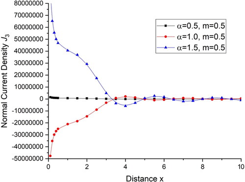
A comparison of the dimensionless form of the field variables displacement components, normal force stress$t_{zz},$ tangential stress $t_{zx},$ temperature T, the current density components $J_1$ and $J_3$ for a transversely isotropic magneto-thermoelastic medium with the same value of hall current parameter and varying fractional order parameter is demonstrated graphically as:

1. The black line with square symbol relates to hall current for $m=0.5\mathit{and}\alpha =0.5,$

2. The red line with circle symbol relates to hall current for $m=0.5\mathit{and}\alpha =1.0,$

3. The blue line with triangle symbol relates to hall current for $m=0.5\mathit{and}\alpha =1.5,$

Figure 1 demonstrates the deviations of the displacement component $u$ with distance x and Figure 2 demonstrates the deviations of the displacement component $w$ with distance x. For all the three values of $\alpha$ the displacement component u and w, first increases for 0$\le x\le 2,$ and then follows an oscillatory pattern for $\alpha =0.5$ while for $\alpha =1.0\mathit{and}\alpha =1.5$ deviations are very small and the value of displacement decreases with increase in the value of distance x. Figure 3 demonstrates the deviations of temperature T with distance x. There is a sharp decrease in the value of temperature in the initial range of distance x when$\alpha =0.5$ and then follows a small oscillatory pattern while for $\alpha =1.0\mathit{and}\alpha =1.5.$ deviations are very small. Figure 4 illustrates the deviations of tangential stress $t_{zx}$ with distance x and Figure 5 shows the deviations of normal stress $t_{zz}$ with distance x. 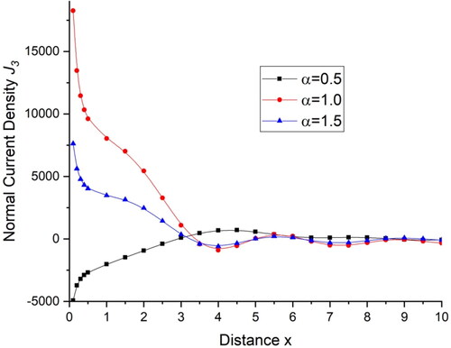For the initial range$0\le x\le 4$ there is a sharp increase in the value of tangential stress $t_{zx}$ and normal stress $t_{zz}$ for the fractional order parameter $\alpha =0.5\mathit{and}\alpha =1.0$ and then follow an oscillatory pattern while for $\alpha =1.5$ there is a small change in the values. Figure 6 displays the deviations current density components $J_1$ and Figure 7 shows the current density components $J_3$ with distance x. There is a sharp decrease in the value of current density components $J_1$ within the initial range of distance x, for $\alpha =0.5$ then follows a small oscillatory pattern while for the initial range of distance x the current density components $J_3$ first increases and then remains almost the same with little variations in the value.

Figure 1. Variations of displacement component u with distance x.

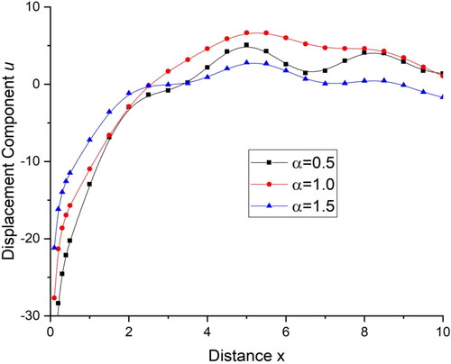
Figure 2. Variations of displacement component w with distance x.

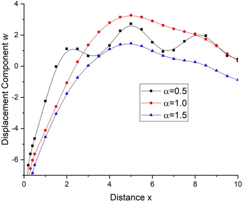
Figure 3. Variations of temperature T with distance x.

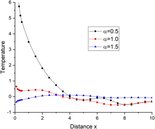
Figure 4. Variations of tangential stress t_zx with distance x.

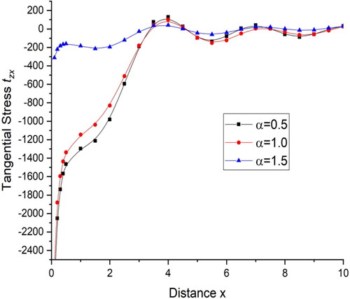
Figure 5. Variations of the normal stress component $t_{zz}$ with distance x.

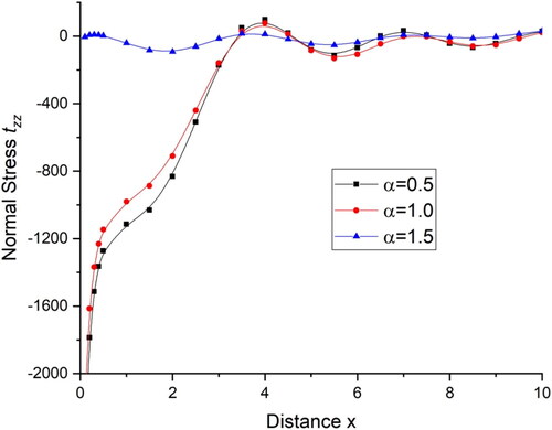
Figure 6. Variations of transverse current density J₁ with distance x.

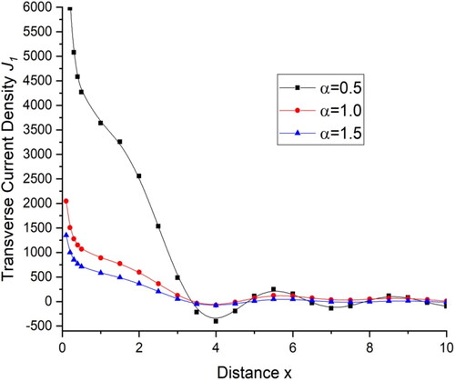
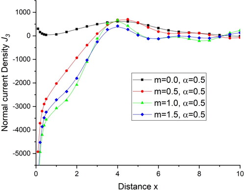
Figure 7. Variations of normal current density J₃ with distance x.

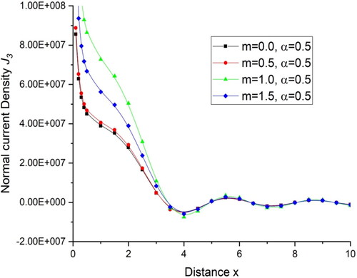
A comparison of the dimensionless form of the field variables displacement components u and w, normal force stress$t_{zz},$ tangential stress $t_{zx},$ temperature T, the current density components $J_1$ and $J_3$ for a transversely isotropic magneto-thermoelastic medium with varying hall current parameter and the same value of fractional order parameter is demonstrated graphically as:

1. The black line with square symbol relates to hall current for $m=0.0\mathit{and}\alpha =0.5,$

2. The red line with circle symbol relates to hall current for $m=0.5\mathit{and}\alpha =0.5,$

3. The green line with triangle symbol relates to hall current for $m=1.0\mathit{and}\alpha =0.5,$

4. The blue line with rhombus symbol relates to hall current for $m=1.5\mathit{and}\alpha =0.5.$

Figure 8 demonstrates the deviations of the displacement component $u$ with distance x. For the initial range of distance x, i.e., for $0\le x\le 2$ and for hall current parameter $m=0.0,m=0.5\mathit{and}m=1.0$ the displacement component u, first increases while for m = 1.5 there is a small increase, and then follows an oscillatory pattern for all the four cases with the almost same amplitude. Figure 9 demonstrates the deviations of the displacement component $w$ with distance x. For the initial range of distance, $0\le x\le 2,$ there is a sudden increase in the value of displacement component w for m = 0.0 and m = 0.5 while for m = 1.0 there is small decrease in the value of displacement component w for this range of distance and for m = 1.5 there is sudden decrease in the value of displacement component w for this range of distance and oscillatory pattern is followed for all the four cases for rest of the distance x. Figure 10 demonstrates the deviations of temperature T with distance x. There is a sharp decrease in the value of temperature T in the initial range of distance x, i.e., for $0\le x\le 4$ for hall parameter$m=0.0,m=0.5\mathit{and}m=1.0$ and then follows a small oscillatory pattern while for m = 1.5 it simply follows the oscillatory pattern. Figure 11 illustrates the deviations of tangential stress $t_{zx}$ with distance x and Figure 12 shows the deviations of normal stress $t_{zz}$ with distance x For the initial range$0\le x\le 4$ there is a sharp increase in the value of tangential stress $t_{zx}$ and normal stress $t_{zz}$ for all the four cases and then follow the oscillatory pattern. Figure 13 displays the deviations of current density components $J_1$ and Figure 14 shows the current density components $J_3$ with distance x. There is a sharp decrease in the value of current density components $J_1$ within the initial range of distance x, $0\le x\le 3$ for all the four cases and then follows oscillatory pattern with little amplitude difference while for the initial range of distance x the current density components $J_3$ first increases for $m=0.5,m=1.0\mathit{and}m=1.5$ and then remains almost the same with little variations in the amplitude of oscillations and for m = 0.0 there are almost the same values with a negligible difference.

Figure 8. Variations of displacement component u with distance x.

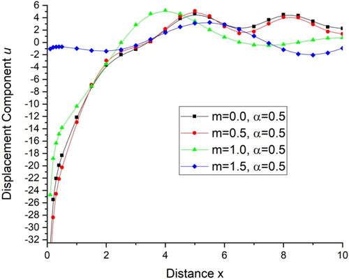
Figure 9. Variations of displacement component w with distance x.

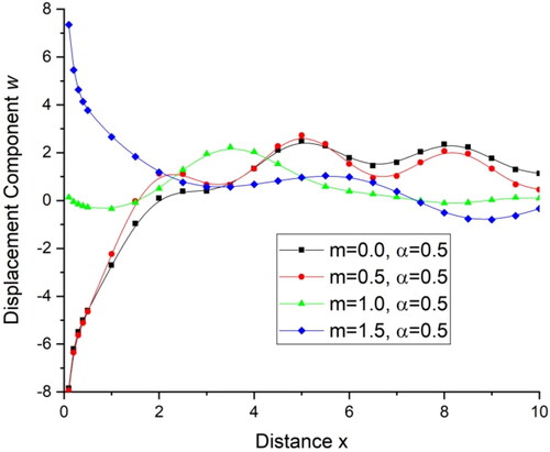
Figure 10. Variations of temperature T with distance x.

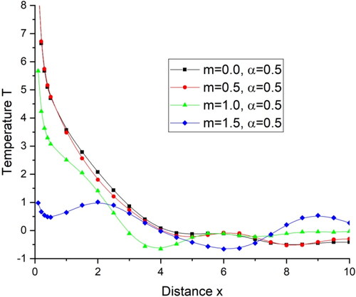
Figure 11. Variations of tangential stress t_zx with distance x.

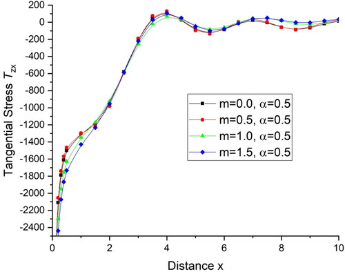
Figure 12. Variations of the normal stress component $t_{zz}$ with distance x.

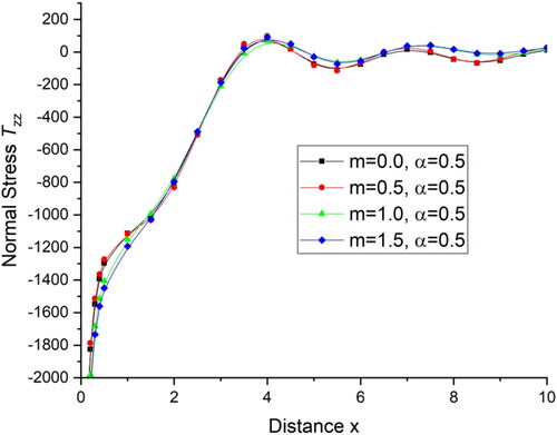
Figure 13. Variations of transverse current density J₁ distance x.

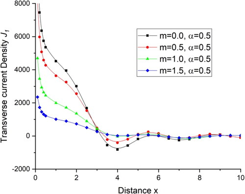
Figure 14. Variations of normal current density J₃ distance x.

Case II Thermal force

A comparison of the dimensionless form of the field variables displacement components, normal force stress$t_{zz},$ tangential stress $t_{zx},$ radial stress, temperature T for a transversely isotropic plate with hall current and fractional order parameter is demonstrated graphically as:

1. The black line with square symbol relates to hall current for $m=0.5\mathit{and}\alpha =0.5,$

2. The red line with circle symbol relates to hall current for $m=0.5\mathit{and}\alpha =0.1,$

3. The blue line with triangle symbol relates to hall current for $m=0.5\mathit{and}\alpha =1.5,$

Figure 15 demonstrates the deviations of the displacement component $u$ with distance x and Figure 16 demonstrates the deviations of the displacement component $w$ with distance x. For the fractional order parameter $\alpha =0.5\mathit{and}\alpha =1.0$ the displacement component u and w, first decreases for 0$\le x\le 4,$ and then remains almost same for rest of the range while for $\alpha =1.5$ for the initial range of distance x, i.e., for 0$\le x\le 4$ the value of displacement increases and oscillates for rest of the range. Figure 17 demonstrates the deviations of temperature T with distance x. There is a sharp decrease in the value of temperature in the initial range of distance x, i.e., for 0$\le x\le 4$ when$\alpha =1.0$ and then follows a small oscillatory pattern while for $\alpha =0.5\mathit{and}\alpha =1.5.$ there is an increase in the value of temperature in the initial range of distance x, i.e., for 0$\le x\le 4$ and then follows the small oscillatory pattern. Figure 18 illustrates the deviations of tangential stress $t_{zx}$ with distance x. For $\alpha =0.5$ and for 0$\le x\le 4$ the tangential stress $t_{zx}$ first increases and then remains almost the same while for$\alpha =1.0\mathit{and}\alpha =1.5$ the tangential stress $t_{zx}$ first decreases and for 0$\le x\le 4$ and then follow oscillatory pattern Figure 19 shows the deviations of normal stress $t_{zz}$ with distance x. For the initial range$0\le x\le 4$ there is a sharp increase in the value of normal stress $t_{zz}$ for the fractional order parameter $\alpha =0.5\mathit{and}\alpha =1.0$ and then follow an oscillatory pattern while for $\alpha =1.5$ there is a sharp decrease in the value of normal stress $t_{zz}$ and then follow the oscillatory pattern. Figure 20 displays the deviations current density components $J_1$ There is a sharp decrease in the value of current density components $J_1$ within the initial range of distance x, for $\alpha =0.5$ then remains almost same for rest of the range of distance x while for$\alpha =1.0$ For the initial range$0\le x\le 4$ there is a slight increase in the value of current density components $J_1$ remains almost the same for rest of the range of distance x and for$\alpha =1.5$ For the initial range$0\le x\le 4$ there is a sudden increase in the value of current density components $J_1$ and for the rest of the range of distance x follows the small oscillatory pattern. Figure 21 shows the current density components $J_3$ with distance x. and then for the current density components $J_3$ for $\alpha =0.5$ remains almost same for all the range of distance x the current density components $J_3$ first increases for $\alpha =1.0$ and the current density components $J_3$ first decreases for $\alpha =1.5$ For the initial range$0\le x\le 4$ then and for the rest of the range of distance x follows the small oscillatory pattern.

Figure 15. Variations of displacement component u with distance x.

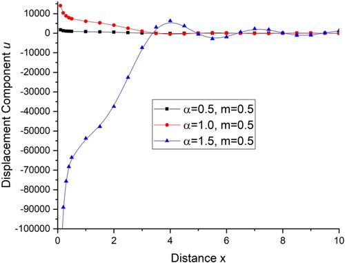
Figure 16. Variations of displacement component w with distance x.

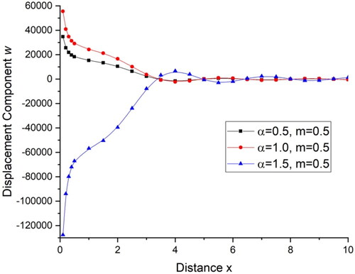
Figure 17. Variations of temperature T with distance x.

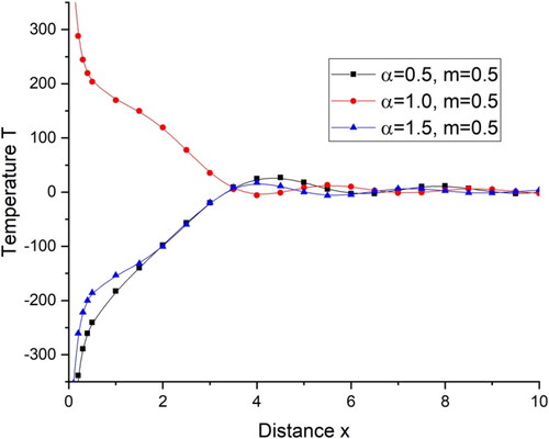
Figure 18. Variations of tangential stress t_zx with distance x.

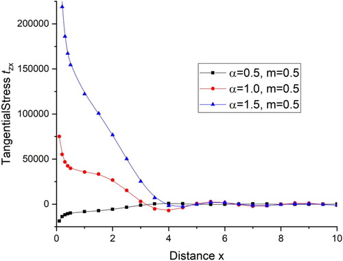
Figure 19. Variations of the normal stress component $t_{zz}$ with distance x.

Figure 20. Variations of transverse current density J₁ distance x.

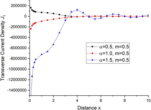
Figure 21. Variations of normal current density J₃ distance x.

A comparison of the dimensionless form of the field variables displacement components u and w, normal force stress$t_{zz},$ tangential stress $t_{zx},$ temperature T, the current density components $J_1$ and $J_3$ for a transversely isotropic magneto-thermoelastic medium for thermal sources with varying hall current parameter and the same value of fractional order parameter is demonstrated graphically as:

1. The black line with square symbol relates to hall current for $m=0.0\mathit{and}\alpha =0.5,$

2. The red line with circle symbol relates to hall current for $m=0.5\mathit{and}\alpha =0.5,$

3. The green line with triangle symbol relates to hall current for $m=1.0\mathit{and}\alpha =0.5,$

4. The blue line with rhombus symbol relates to hall current for $m=1.5\mathit{and}\alpha =0.5.$

Figure 22 demonstrates the deviations of the displacement component $u$ with distance x and Figure 23 demonstrates the deviations of the displacement component $w$ with distance x. For the initial range of distance x, i.e., for $0\le x\le 4$ and for hall current parameter $m=0.0\mathit{and}m=0.5$ for the value of the displacement component u and w, there is sudden increase while for m = 1.0 and m = 1.5 there is sudden decrease, and then follows oscillatory pattern for all the four cases with almost some amplitude difference. Figure 24 demonstrates the deviations of temperature T with distance x. For the initial range of distance x, i.e., for $0\le x\le 4$ and for hall current parameter $m=0.0\mathit{and}m=0.5$ for the value of temperature T, there is sudden increase while for m = 1.0 and m = 1.5 there is sudden decrease, and then follows an oscillatory pattern for all the four cases with almost some amplitude difference. Figure 25 illustrates the deviations of tangential stress $t_{zx}$ with distance x For the initial range$0\le x\le 4$ there is a sharp increase in the value of tangential stress $t_{zx}$ for all the four cases and then have the same value for the rest of the distance x. and Figure 26 shows the deviations of normal stress $t_{zz}$ with distance x. For the initial range$0\le x\le 4$ there is a sharp decrease in the value of normal stress $t_{zz}$ for all the four cases and then follows an oscillatory pattern for the rest of the range. Figure 27 displays the deviations of current density components $J_1.$ There is a sharp increase in the value of current density components $J_1$ in the initial range of distance x, $0\le x\le 3$ for m = 0.0 and m = 0.5 and then follows oscillatory pattern with little amplitude difference while for m = 0.5 the value of current density components $J_1$ remains almost the same for any distance x. And for m = 1.5 there is a sharp decrease in the value of current density components $J_1$ in the initial range of distance x, $0\le x\le 3$ and then follows oscillatory pattern Figure 28 shows the current density components $J_3$ with distance x. For the initial range of distance x, $0\le x\le 4$ the current density components $J_3$ first decreases all the four cases and then oscillates with the almost same amplitude.

Figure 22. Variations of displacement component u with distance x.

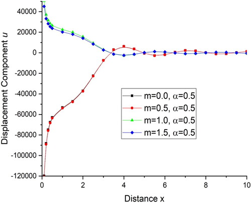
Figure 23. Variations of displacement component w with distance x.

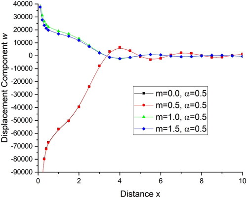
Figure 24. Variations of temperature T with distance x.

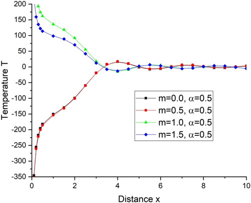
Figure 25. Variations of tangential stress t_zx with distance x.

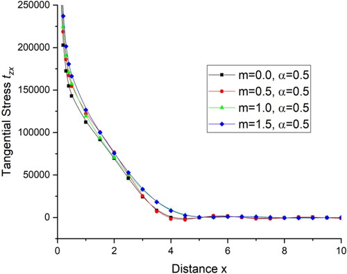
Figure 26. Variations of the normal stress component $t_{zz}$ with distance x.

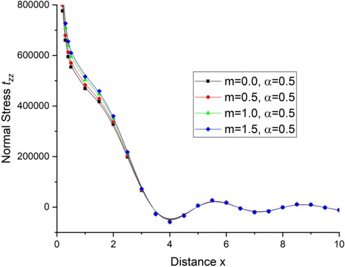
Figure 27. Variations of transverse current density J₁ distance x.

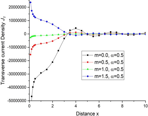
Figure 28. Variations of normal current density J₃ distance x.

8. Conclusion

From the analysis of the graphs, it is clear that the mathematical model for hall current effect in homogeneous transversely isotropic magneto thermoelastic (HTIMT) rotating medium with fractional order heat transfer has been investigated. Results are illustrated in the forms of graphs with fractional order heat transfer and Hall current. There is a significant influence of Hall Effect parameter m, and fractional order parameter $\alpha$ on the deformation of various displacement components, temperature, tangential stress components, and current density components $J_1$ and $J_3$ of HTIMT medium. As distance x, varied from the point of use of the normal force, the variations of displacement components, temperature, and tangential stress components undergo sudden changes, causing inconsistent patterns of curves under weak, normal and strong conductivity. The shape of curves shows the impact of fractional order parameter with fixed values of Hall Effect parameter m on the body and fulfills the purpose of the study. The outcomes of this research are extremely helpful in the 2-D problem with dynamic response of thermomechanical interactions with fractional order heat transfer in transversely isotropic thermoelastic solid and resulting formulation is applied to a semi-infinite electrically perfect conducting half-space of elastic solids in the presence of a constant magnetic field and beneficial for researchers working in material science as well as for those working on the development of magneto-thermoelasticity and in practical situations, such as in high-energy particle accelerators, geophysics and geomagnetic. The methods used in the present article are applicable to a wide range of problems in thermodynamics and thermoelasticity.

References

- Abbas, I. (2018). A study on fractional order theory in thermoelastic half-space under thermal loading. Physical Mesomechanics, 21(2), 150–156.
- Abbas, I. A., & Youssef, H. M. (2009). Finite element analysis of two-temperature generalized magnetothermoelasticity. Archive of Applied Mechanics, 79(10), 917–925. doi:10.1007/s00419-008-0259-9
- Abbas, I. A., & Youssef, H. M. (2013). Two-temperature generalized thermoelasticity under ramp-type heating by finite. Meccanica, 48(2), 331–339. doi:10.1007/s11012-012-9604-8
- Bachher, M., & Sarkar, N. (2016). Fractional order magneto-thermoelasticity in a rotating media with one relaxation time. Mathematical Models in Engineering, 2(1), 56–68.
- Caputo, M. (1967). Linear models of dissipation whose Q is almost frequency independent—II. Geophysical Journal International, 13(5), 529–539. doi:10.1111/j.1365-246X.1967.tb02303.x
- Dhaliwal, R. S., & Sherief, H. H. (1980). Generalized thermoelasticity for anisotropic media. Quarterly of Applied Mathematics, XXXVII(1), 1–8. doi:10.1090/qam/575828
- Elsafty, M. (2015). A half-space problem in the theory of fractional order thermoelasticity with diffusion. IJSER, 6, 358–371.
- Ezzat, M. A., & El-Bary, A. A. (2016). Effects of variable thermal conductivity and fractional order of heat transfer on a perfect conducting infinitely long hollow cylinder. International Journal of Thermal Sciences, 108, 62–69. doi:10.1016/j.ijthermalsci.2016.04.020
- Ezzat, M. A., & El-Bary, A. A. (2017). Fractional magneto-thermoelastic materials with phase lag Green-Naghdi theories. Steel and Composite Structures, 24(3), 297–307.
- Ezzat, M. A., El-Karamany, A. S., & El-Bary, A. A. (2018). Two-temperature theory in Green–Naghdi thermoelasticity with fractional phase-lag heat transfer. Microsystem Technologies, 24(2), 951–961. doi:10.1007/s00542-017-3425-6
- Ezzat, M. A., El-Karamany, A. S., & Ezzat, S. M. (2012). Two-temperature theory in magneto-thermoelasticity with fractional order dual-phase-lag heat transfer. Nuclear Engineering and Design, 252, 267–277. doi:10.1016/j.nucengdes.2012.06.012
- Ezzat, M. A., El-Karamany, A. S., & Fayik, M. A. (2012). Fractional order theory in thermoelastic solid with three-phase lag heat transfer. Archive of Applied Mechanics, 82(4), 557–572. doi:10.1007/s00419-011-0572-6
- Green, A. E., & Naghdi, P. M. (1992). On undamped heat waves in an elastic solid. Journal of Thermal Stresses, 15(2), 253–264. doi:10.1080/01495739208946136
- Honig, G., & Hirdes, U. (1984). A method for the numerical inversion of Laplace transform. Journal of Computational and Applied Mathematics, 10(1), 113–132. doi:10.1016/0377-0427(84)90075-X
- Kaur, I., & Lata, P. (2019a). Effect of hall current on propagation of plane wave in transversely isotropic thermoelastic medium with two temperature and fractional order heat transfer. SN Applied Sciences, 1(8), 900. doi:10.1007/s42452-019-0942-1
- Kaur, I., & Lata, P. (2019b). Transversely isotropic thermoelastic thin circular plate with constant and periodically varying load and heat source. International Journal of Mechanical and Materials Engineering, 14(1), 1–13. doi:10.1186/s40712-019-0107-4
- Kaur, I., & Lata, P. (2019c). Rayleigh wave propagation in transversely isotropic magneto thermoelastic medium with three phase lag heat transfer and diffusion. International Journal of Mechanical and Materials Engineering, 14(1), 1–11. doi:10.1186/s40712-019-0108-3
- Kumar, R., Sharma, N., & Lata, P. (2016a). Thermomechanical interactions in transversely isotropic magnetothermoelastic medium with vacuum and with and without energy dissipation with combined effects of rotation, vacuum and two temperatures. Applied Mathematical Modelling, 40(13–14), 6560–6575. doi:10.1016/j.apm.2016.01.061
- Kumar, R., Sharma, N., & Lata, P. (2016b). Thermomechanical interactions due to hall current in transversely isotropic thermoelastic with and without energy dissipation with two temperatures and rotation. Journal of Solid Mechanics, 8(4), 840–858.
- Kumar, R., Sharma, N., & Lata, P. (2017). Effects of Hall current and two temperatures intransversely isotropic magnetothermoelastic with and without energy dissipation due to ramp-type heat. Mechanics of Advanced Materials and Structures, 24(8), 625–635. doi:10.1080/15376494.2016.1196769
- Lata, P. (2017). A comparison between isotropic and transversely isotropic thermoelastic solids with two temperature and without energy dissipation in frequency domain due to concentrated force. International Journal of Mechanics and Solids, 9(1), 77–88.
- Lata, P., & Kaur, I. (2018). Effect of hall current in transversely isotropic magnetothermoelastic rotating medium with fractional order heat transfer due to normal force. Advances in Materials Research, 7(3), 203–220.
- Lata, P., & Kaur, I. (2019a). Plane wave propagation in transversely isotropic magnetothermoelastic rotating medium with fractional order generalized heat transfer. Structural Monitoring and Maintenance, 6(3), 191–218. doi:10.12989/smm.2019.6.3.191
- Lata, P., & Kaur, I. (2019b). Transversely isotropic thermoelastic thin circular plate with time harmonic sources. Geomechanics and Engineering, 19(1), 29–36. doi:10.12989/gae.2019.19.1.029
- Mahmoud, S. (2012). Influence of rotation and generalized magneto-thermoelastic on Rayleigh waves in a granular medium under effect of initial stress and gravity field. Meccanica, 47(7), 1561–1579. doi:10.1007/s11012-011-9535-9
- Mahmoud, S. R., Abd-Alla, A. M., & El-Sheikh, M. A. (2011). Effect of the rotation on wave motion through cylindrical bore in a micropolar porous medium. International Journal of Modern Physics B, 25(20), 2713–2728. doi:10.1142/S0217979211101739
- Mahmoud, S. R., Marin, M., & Al-Basyouni, K.S. (2015). Effect of the initial stress and rotation on free vibrations in transversely isotropic human long dry bone. Analele Universitatii “Ovidius” Constanta-Seria Matematica, 23(1), 171–184. doi:10.1515/auom-2015-0011
- Marin, M., Baleanu, D., & Vlase, S. (2017). Effect of microtemperatures for micropolar thermoelastic bodies. Structural Engineering and Mechanics, 61(3), 381–387. doi:10.12989/sem.2017.61.3.381
- Moreno-Navarro, P., Ibrahimbegovic, A., & Pérez-Aparicio, J. L. (2018). Linear elastic mechanical system interacting with coupled thermo-electro-magnetic fields. Coupled Systems Mechanics, 7(1), 5–25.
- Press, W. T. (1986). Numerical recipes in Fortran. Cambridge: Cambridge University Press.
- Schoenberg, M., & Censor, D. (1973). Elastic waves in rotating media. Quarterly of Applied Mathematics, 31(1), 115–125. doi:10.1090/qam/99708
- Sheoran, S. S., & Kundu, P. (2016). Fractional order generalized thermoelasticity theories: A review. International Journal of Advances in Applied Mathematics and Mechanics, 3(4), 76–81.
- Sherief, H. H., & Hamza, F. A. (2016). Modeling of variable thermal conductivity in a generalized thermoelastic infinitely long hollow cylinder. Meccanica, 51(3), 551–558. doi:10.1007/s11012-015-0219-8
- Sherief, H., & El-Latief, A. M. (2013). Effect of variable thermal conductivity on a half-space under the fractional order theory of thermoelasticity. International Journal of Mechanical Sciences, 74, 185–189. doi:10.1016/j.ijmecsci.2013.05.016
- Slaughter, W. (2002). The linearised theory of elasticity. Basel: Birkhausar.
- Tripathi, J.J., Deshmukh, K., & Verma, J. (2017). Fractional order generalized thermoelastic problem in a thick circular plate with periodically varying heat source. International Journal of Thermodynamics, 20(3), 132–138. doi:10.5541/eoguijt.336651
- Youssef, H. M., & Abbas, I. (2014). Fractional order generalized thermoelasticity with variable thermal conductivity. Journal of Vibroengineering, 16(8), 4077–4087.
- Zakaria, M. (2012). Effects of hall current and rotation on magneto-micropolar generalized thermoelasticity due to ramp-type heating. International Journal of Electromagnetics and Applications, 2(3), 24–32.