Reliable iterative methods for 1D Swift–Hohenberg equation

Abstract

In this paper, the nonlinear problem of the 1 D Swift-Hohenberg equation (S-HE) has been solved by using five reliable iterative methods. The first one is the Daftardar-Jafari method namely (DJM), the second method is the Temimi-Ansari method namely (TAM), the third method is the Banach contraction method namely (BCM), the fourth method is the Adomian decomposition method namely (ADM) and finally the fifth method is the Variational iteration method (VIM) to obtain the approximate solutions. In this work, we discussed and applied these iterative methods to solve the S-HE and compared them. In addition, the fixed-point theorem was given to illustrate the convergence of the five methods. To illustrate the accuracy and efficiency of the five methods, the maximum error remainder was calculated since the exact solution is unknown. The results showed that the five iterative methods are accurate, reliable, time saver and effective. All the iterative processes in this paper implemented in MATHEMATICA®11.

Keywords:

• Approximate solution
• iterative methods
• nonlinear partial differential equations
• semi-analytical solution
• Swift-Hohenberg equation

1. Introduction

There are many natural phenomena in engineering and applied sciences are modeled by either linear or nonlinear ordinary\partial differential equations, hence that solution of these equations is very important. Numerous nonlinear problems that arising in various engineering applications have no exact solution or cannot be obtainable. Therefore, there is always demand to develop reliable and efficient methods to get an approximate solution of these equations (Al-Jawary, 2016, 2017; Mitlif, 2014; Sahib & Hasan, 2014; Yin, Kumar, & Kumar, 2015).

In 1977, the Swift and Hohenberg (1977) derived a partial differential equation named as the S-HE from the thermal convection equations. The S-HE occurs fundamentally in nanocrystalline materials by describing the average density of dissociation under the formation of shear microbands (Kudryashov & Ryabov, 2016). It has been widely applied as a model for the study of numerous issues in pattern formation, such as the effects of noise on bifurcations, pattern selection, spatiotemporal chaos, the dynamics of defects, model patterns in Rayleigh-Bernard convection, biological materials, like neural tissues and in the study of lasers (Chossat & Faye, 2015; Kubstrup, Herrero, & Pérez-García, 1996; Peletier & Rottschäfer, 2004; Pérez-Moreno, Chavarría, & Chavarría, 2014).

Furthermore, some analytic and approximate methods have been used and implemented to solve the S-HE such as, homotopy perturbation method (HPM) (Ban & Cui, 2018), shooting method (Tao & Zhang, 2002), homotopy analysis method (HAM) (Akyildiz, Siginer, Vajravelu, & Van Gorder, 2010), Reproducing kernel method (Bakhtiari, Abbasbandy, & Van Gorder, 2018).

In 2011, Wang and Yanti introduced an efficient time-splitting Fourier spectral method to solve this equation (Wang & Yanti, 2011). In addition, Deng and Li used a classical Lyapunov-Schmidt method, a perturbation method and a fixed-point theorem to solve the S-HE (Deng & Li, 2012). He’s semi-inverse method has been used to introduce the solitary wave solution of the S-HE (Fonseca, 2017).

In this paper, the five semi-analytical iterative methods will be implemented to solve the S-HE to get an approximate solution. The first one is the DJM suggested by Daftardar-Gejji and Jafari in 2006 (Daftardar-Gejji & Jafari, 2006), the second method is the TAM introduced by Temimi and Ansari (2011a, 2011b), the third method is the BCM presented by Daftardar-Gejji and Bhalekar in 2009 (Daftardar-Gejji & Bhalekar, 2009), the fourth method is the ADM, it was introduced by George Adomian in the beginning of 1980 (Adomian, 1994) and finally the fifth method is the VIM introduced by Ji-Huan He in 1999 (He, 1999).

These iterative methods have been successfully used to solve different types of non-linear ordinary and partial differential equations for more details, see (Abdul Nabi & Al-Jawary, 2018; Akbarzade & Langari, 2011; Al-Jawary, Adwan, & Radhi, 2020; Al-Jawary, Azeez, & Radhi, 2018; Al-Jawary, Radhi, & Ravnik, 2017, 2018; Al-Jawary & Raham, 2017; Ateeah, 2017; Razzaq & Yassein, 2017; Wazwaz, 2000; Zhu, Chang, & Wu, 2005).

This paper has been organized as follows: In section 2, the S-HE formulation will be presented. The basic concepts of five iterative methods will be presented and discussed in section 3. In section 4, solving S-HE using the DJM, TAM, BCM, ADM and VIM will be given. The convergence of the proposed techniques will be explained in section 5. In section 6, the numerical simulations and discussion are introduced and finally, the conclusion will be given in section 7.

2. The nonlinear S-HE

The following nonlinear partial differential equation presents the S-HE as a model for the study of pattern formation, in connection with the Rayleigh-Bernard convection (Haragus & Scheel, 2007; Peletier & Williams, 2007). (1) $$\frac{\partial v}{\partial t}=-{\left(\frac{{\partial }^2}{{\partial x}^2}+1\right)}^{2}v+\alpha v-v^3,\mathrm{ }$$(1) with the following boundary and initial conditions: $$v\left(0,t\right)=v\left(1,t\right)=0,\mathrm{ }{v}_{xx}\left(0,t\right)=v_{xx}\left(1,t\right)=0,\mathrm{ }v\left(x,0\right)=v_0\left(x\right).$$ where$\mathrm{ }v\left(x,t\right)\mathrm{ }$ is the scalar function with two independent variables defined on the line or the plane, $\alpha$ is real bifurcation parameter, $x\in [0,1],$ $t>0\mathrm{ }$ and $v_0\left(x\right)$ is a smooth function.

One can write the Equation (1)(1) $$\frac{\partial v}{\partial t}=-{\left(\frac{{\partial }^2}{{\partial x}^2}+1\right)}^{2}v+\alpha v-v^3,\mathrm{ }$$(1) in a more conventional form as: (2) $$v_t=-v_{\mathit{xxxx}}-2v_{xx}-\left(1-\alpha \right)v-f\left(v\right),\mathrm{for}\mathrm{ }0<x<L, t>0$$(2) and the initial condition: (3) $$v\left(0,t\right)=v_{xx}\left(0,t\right)=0\text{ and }v \left(x,0\right)=A\text{sin}\left[\frac{\pi x}{L}\right].$$(3) where, $f\left(v\right)=v^3,$ is some smooth nonlinearity, $L$ length of domain and$\mathrm{ }A=\frac{1}{10},$ as given in (Peletier & Rottschäfer, 2004).

3. The basic concepts of the iterative methods

In this section, the basic idea of the suggested five iterative methods: DJM, TAM, BCM, ADM and VIM will be introduced.

3.1 The basic steps of the DJM

Daftardar-Gejji and Jafari have supposed the following nonlinear functional equation (Bhalekar & Daftardar-Gejji, 2008; Daftardar-Gejji & Bhalekar, 2010; Daftardar-Gejji & Jafari, 2006). (4) $$v=f+L\left(v\right)+N\left(v\right),\mathrm{ }$$(4) where $L$ and$\mathrm{ }N$ represent are linear and nonlinear operators, respectively, $f$ is a known function and $v\mathrm{ }$ is an unknown function.

We are looking for a solution $v$ of Equation (4)(4) $$v=f+L\left(v\right)+N\left(v\right),\mathrm{ }$$(4) and can be obtained by the following series: $$v=\sum _{k=0}^{\mathrm{\infty }}{v}_k$$

Because $L$ is linear operator then: $$L\left({\sum }_{k=0}^{\mathrm{\infty }}{v}_k\right)=\sum _{k=0}^{\mathrm{\infty }}L(v_k)$$

Therefore, Equation (4)(4) $$v=f+L\left(v\right)+N\left(v\right),\mathrm{ }$$(4) can be written as: $$\sum _{k=0}^{\mathrm{\infty }}{v}_k=f+\sum _{k=0}^{\mathrm{\infty }}L(v_k)+N\left(\sum _{k=0}^{\mathrm{\infty }}{v}_k\right)$$ and the nonlinear operator $N$ can be decomposed as bellow: $$N\left({\sum }_{k=0}^{\mathrm{\infty }}{v}_k\right)=N\left(v_0\right)+{\sum }_{i=1}^{\mathrm{\infty }}\left\{N\left({\sum }_{k=0}^i{v}_k\right)-N\left({\sum }_{k=0}^{i-1}{v}_k\right)\right\}$$

Now, let us define the relation as below: $$D_0=N\left(v_0\right),$$ $$D_1=N\left(v_0+v_1\right)-N\left(v_0\right)$$ $$D_2=N\left(v_0+v_1+v_2\right)-N\left(v_0+v_1\right)$$ $$⋮$$ $$D_i=\left\{N\left({\sum }_{k=0}^i{v}_k\right)-N\left({\sum }_{k=0}^{i-1}{v}_k\right)\right\},\mathrm{ }i\ge 1$$

From the above relation we get: $$N\left(\sum _{k=0}^{\mathrm{\infty }}{v}_k\right)=D_0+D_1+D_2+\dots +D_i+\dots$$

By taking the inverse operator, $L^{-1}\left(·\right)={\int }_0^t\left(·\right)d\tau ,$ for both sides of Equation (4)(4) $$v=f+L\left(v\right)+N\left(v\right),\mathrm{ }$$(4) , and using the initial conditions, we get: $$\sum _{k=0}^{\mathrm{\infty }}{v}_k=p+L^{-1}\left(N\left(\sum _{k=0}^{\mathrm{\infty }}{v}_k\right)\right),$$ where$\mathrm{ }p$ represents the final formula for $L^{-1}(f)$ with the given initial conditions.

Therefore, the components of the solution$\mathrm{ }v$ are: (5) $$\begin{array}{l}{v}_0\mathrm{ }=p\\ v_1\mathrm{ }=L^{-1}\left(D_0\right)\\ \begin{array}{l}{v}_2\mathrm{ }=L^{-1}\left(D_1\right)\\ \begin{array}{c}⋮\\ v_{k+1}=L^{-1}\left(D_k\right),\mathrm{ }k=0,1,2,\dots \end{array}\end{array}\end{array}$$(5)

As a result, the n-term approximate solution of Equation (4)(4) $$v=f+L\left(v\right)+N\left(v\right),\mathrm{ }$$(4) is given by the following form: $${\psi }_n=\sum _{i=0}^n{v}_i$$

Finally, the solution$\mathrm{ }v(x,t)$ for the nonlinear problem is given by: (6) $$v(x,t)=\sum _{k=0}^{\mathrm{\infty }}{v}_k$$(6)

3.2 The basic idea of the TAM

Temimi and Ansari have presented the semi-analytical an iterative method namely) TAM (for solving nonlinear differential equations (Temimi & Ansari, 2011a, 2011b, 2015).

To illustrate the basic ideas of the suggested method, let us consider the general form of partial differential equation: (7) $$L\left(v\left(x,t\right)\right)+N\left(v\left(x,t\right)\right)+f=0\mathrm{ }$$(7) with boundary condition: $B\left(v,\frac{\partial v}{\partial x}\right)=0,$ where$\mathrm{ }L$ is a linear operator, $N$ is a nonlinear operator, $(x,\mathrm{ }t)$ denotes the independent variables, $v\left(x,t\right)$ is an unknown function, $f\mathrm{ }$ is a known function and $B$ is a boundary operator.

Now, we begin by assuming that $v_0\left(x,t\right)$ is an initial approximation of the problem $v\left(x,t\right)$ through solving the following initial equation: $$L\left(v_0(x,t)\right)+f=0\text{ with }B\left(v_0,\frac{\partial v_0}{\partial x}\right)=0$$

To obtain the next iteration $v_1\left(x,t\right)$ to the solution$\mathrm{ }v\left(x,t\right),$ we must solve the following equation: $$L\left(v_1(x,t)\right)+f+N\left(v_0\left(x,t\right)\right)=0\text{ with }B\left(v_1,\frac{\partial v_1}{\partial x}\right)=0,$$

Similarly, all iterations $v_{n+1}(x,t)$ can be obtained as: (8) $$L\left(v_{n+1}(x,t)\right)+f+N\left(v_n\left(x,t\right)\right)=0\text{ with }B\left(v_{n+1},\frac{\partial v_{n+1}}{\partial x}\right)=0,\mathrm{ }$$(8)

Note that each of them $v_n(x,t)$ is a solution to Equation (7)(7) $$L\left(v\left(x,t\right)\right)+N\left(v\left(x,t\right)\right)+f=0\mathrm{ }$$(7) . Also, by increasing the iterations, a better accuracy for the approximate solution will be obtained.

So, the solution for the Equation (7)(7) $$L\left(v\left(x,t\right)\right)+N\left(v\left(x,t\right)\right)+f=0\mathrm{ }$$(7) is given by: (9) $$v\left(x,t\right)=\underset{n\to \mathrm{\infty }}{\lim }{v}_n\left(x,t\right)\mathrm{ }$$(9)

3.3 The basic idea of BCM

To study the basic idea of the proposed method, we consider the general form of nonlinear functional equation (Daftardar-Gejji & Bhalekar, 2009): (10) $$v=f+N\left(v\right),\mathrm{ }$$(10)

Now, we will define successive approximations as follows: (11) $$\begin{array}{l}\genfrac{}{}{0pt}{}{v_0=f,\mathrm{ }}{\begin{array}{c}{v}_1=v_0+N\left(v_0\right)\\ v_2=v_0+N\left(v_1\right)\\ ⋮\end{array}}\\ v_n=v_0+N\left(v_{n-1}\right),\mathrm{ }n=1,2,\dots \end{array}$$(11)

It has been shown that the series defined by Equation (11)(11) $$\begin{array}{l}\genfrac{}{}{0pt}{}{v_0=f,\mathrm{ }}{\begin{array}{c}{v}_1=v_0+N\left(v_0\right)\\ v_2=v_0+N\left(v_1\right)\\ ⋮\end{array}}\\ v_n=v_0+N\left(v_{n-1}\right),\mathrm{ }n=1,2,\dots \end{array}$$(11) is convergent (Daftardar-Gejji & Bhalekar, 2009). Thus, the solution of Equation (10)(10) $$v=f+N\left(v\right),\mathrm{ }$$(10) is given by: $$v=\underset{n\to \mathrm{\infty }}{\lim }{v}_n$$

3.4 The basic idea of the ADM

George Adomian has presented an iterative method namely (ADM) for solving non-linear differential equations (Adomian, 1994, 2014; Adomian & Rach, 1993). To illustrate the basic ideas of the ADM, let us consider the general form of the partial differential equation: (12) $$L\left(v\right)+R\left(v\right)+N\left(v\right)=f\mathrm{ }$$(12)

Where, $L\left(v\right)+R\left(v\right)$ the linear terms such that $L$ is an invertible linear operator, R is a linear differential operator with order derivative less than L, $N\left(v\right)$ is a nonlinear operator term and $f\mathrm{ }$ is a known function. We begin by assuming the inverse operator for$\mathrm{ }L.$

Hence, Equation (12)(12) $$L\left(v\right)+R\left(v\right)+N\left(v\right)=f\mathrm{ }$$(12) can be written as: (13) $$v=L^{-1}\left(f\right)-L^{-1}\left(R\left(v\right)\right)-L^{-1}\left(N\left(v\right)\right),\mathrm{ }$$(13)

The solution to Equation (13)(13) $$v=L^{-1}\left(f\right)-L^{-1}\left(R\left(v\right)\right)-L^{-1}\left(N\left(v\right)\right),\mathrm{ }$$(13) is represented in the ADM as the following infinite series: (14) $$v=\mathrm{ }\sum _{k=0}^{\mathrm{\infty }}{v}_k\mathrm{ }$$(14)

Assume that the nonlinear operator term$\mathrm{ }N\left(v\right)=\phi \left(v\right)$ is decomposed as: (15) $$\phi \left(v\right)=N\left(v\right)=\sum _{k=0}^{\mathrm{\infty }}{A}_k\mathrm{ }$$(15) where $A_k$ are Adomian’s polynomials, which are represented as in (Adomian, 1994, 2014): (16) $$A_k=\frac{1}{k!}{\left[\frac{{\partial }^k}{\partial {\lambda }^k}F\left(\sum _{i=0}^k{\lambda }^i{v}_i\right)\right]}_{\lambda =0},\mathrm{ }k=0,\mathrm{ }1,\mathrm{ }2,\mathrm{ }\dots \mathrm{ }$$(16)

Now, by substituting the Equations (14)(14) $$v=\mathrm{ }\sum _{k=0}^{\mathrm{\infty }}{v}_k\mathrm{ }$$(14) and (15)(15) $$\phi \left(v\right)=N\left(v\right)=\sum _{k=0}^{\mathrm{\infty }}{A}_k\mathrm{ }$$(15) in Equation (13)(13) $$v=L^{-1}\left(f\right)-L^{-1}\left(R\left(v\right)\right)-L^{-1}\left(N\left(v\right)\right),\mathrm{ }$$(13) , we get the following: (17) $$v=\sum _{k=0}^{\mathrm{\infty }}{v}_k=v_0-L^{-1}(R\left(\sum _{k=0}^{\mathrm{\infty }}{v}_k\right)-L^{-1}\left(\sum _{k=0}^{\mathrm{\infty }}{A}_k\right)\mathrm{ }$$(17)

Thus, it can be composed as: (18) $$\begin{array}{l}{v}_0=\theta +L^{-1}\left(f\right) \\ v_1=-L^{-1}R\left(v_0\right)-L^{-1}\left(A_0\right),\\ \begin{array}{l}{v}_2=-L^{-1}R\left(v_1\right)-L^{-1}\left(A_1\right),\\ \begin{array}{c}⋮\\ v_n=-L^{-1}R\left(v_{k-1}\right)-L^{-1}\left(A_{k-1}\right).\mathrm{ }\end{array}\end{array}\end{array}$$(18) where θ is an initial condition.

Hence, the iterations ${\mathrm{ }v}_{k\mathrm{ }}$ are calculated and the general solution of the Equation (12)(12) $$L\left(v\right)+R\left(v\right)+N\left(v\right)=f\mathrm{ }$$(12) is obtained according to the ADM as follows: (19) $$v=\sum _{k=0}^{\mathrm{\infty }}{v}_k.\mathrm{ }$$(19)

3.5 The basic idea of VIM

Ji-Huan He in 1999 has presented the iterative method namely (VIM) for solving non-linear differential equations (He, 1999, 2007). To explain the basic ideas of the VIM, let us consider the general form of partial differential equation: (20) $$L\left(v\right)+N\left(v\right)=f,\mathrm{ }$$(20)

Where, $L$ is a linear operator, $N\mathrm{ }$ is a nonlinear operator term and $f\mathrm{ }$ is an inhomogeneous term.

According to the VIM, we can construct a correction functional as the following form (21) $$v_{k+1}\left(x\right)=v_k\left(x\right)+{\int }_0^t\left[\lambda \left(t\right)\left(L\left(v_k\left(t\right)\right)-N{(\stackrel{\sim }{v}}_k\left(t\right))-f\left(t\right)\right)\right]dt,\mathrm{ }k=0,1,2,\dots \mathrm{ }$$(21) where ${\stackrel{\sim }{v}}_k$ is considered as a restricted variation and λ is a general Lagrange multiplier that is can be identified optimally by the variational theory (He, 2019a, 2019b; He & Sun, 2019) and given by the following general formula when derivative appeared in the given equation (He, 1999): (22) $$\lambda =\frac{({-1)}^k}{\left(k-1\right)!}{\left(t-x\right)}^{k-1},\mathrm{ }k\ge 1.\mathrm{ }$$(22)

Hence, the solution of Equation (20)(20) $$L\left(v\right)+N\left(v\right)=f,\mathrm{ }$$(20) is given by: (23) $$v\left(x\right)=\underset{k\to \mathrm{\infty }}{\mathit{lim}}{v}_k\left(x\right).\mathrm{ }\mathrm{ }$$(23)

4. Solving the S-HE

In this section, we will implement the iterative methods DJM, TAM, BCM, ADM and VIM to solve the nonlinear S-HE to obtain the approximate solution of this equation.

4.1 Solving the S-HE by the DJM

To solve the S-HE by using the DJM, we re-write Equation (1)(1) $$\frac{\partial v}{\partial t}=-{\left(\frac{{\partial }^2}{{\partial x}^2}+1\right)}^{2}v+\alpha v-v^3,\mathrm{ }$$(1) as follows: (24) $$v_t=-v_{\mathit{xxxx}}-2v_{xx}-\left(1-\alpha \right)v-v^3,\mathrm{ }v\left(x,0\right)=\frac{1}{10}\text{sin}\left[\frac{\pi x}{L}\right].\mathrm{ }$$(24)

First of all, to apply the DJM for the S-HE, we choose the operator form of the Equation (24)(24) $$v_t=-v_{\mathit{xxxx}}-2v_{xx}-\left(1-\alpha \right)v-v^3,\mathrm{ }v\left(x,0\right)=\frac{1}{10}\text{sin}\left[\frac{\pi x}{L}\right].\mathrm{ }$$(24) as follows: (25) $$L_t\left(v(x,t)\right)=N\left(v(x,t)\right),\mathrm{ }$$(25)

Where:

$L_t=\frac{\partial }{\partial t}$ and $N\left(v\right)=-v_{\mathit{xxxx}}-2v_{xx}-\left(1-\alpha \right)v-v^3,$ is the nonlinear operator for the S-HE.

Let us assume the inverse operator $L_t^{-1}(·)={\int }_0^t\left(·\right)dt,$ is exists and by take it for both sides of Equation (25)(25) $$L_t\left(v(x,t)\right)=N\left(v(x,t)\right),\mathrm{ }$$(25) leads to: $$L_t^{-1}{L}_t\left(v(x,t)\right)=L_t^{-1}N\left(v(x,t)\right)$$

Also, by using the initial condition, we get: $$v\left(x,t\right)-v\left(x,0\right)=L_t^{-1}N\left(v(x,t)\right).$$

Then: (26) $$v\left(x,t\right)={\frac{1}{10}\text{sin}\left[\frac{\pi x}{L}\right]+L}_t^{-1}N\left(v(x,t)\right).\mathrm{ }$$(26)

Finally, according to the DJM for Equation (26)(26) $$v\left(x,t\right)={\frac{1}{10}\text{sin}\left[\frac{\pi x}{L}\right]+L}_t^{-1}N\left(v(x,t)\right).\mathrm{ }$$(26) and by applying the recurrence relation, we achieve the components $v_n\left(x,t\right)$ as the following form: $$\begin{array}{l}{v}_0\left(x,t\right)=\frac{1}{10}\mathrm{S}\mathrm{in}\left[\frac{\pi x}{L}\right]\\ v_1\left(x,t\right)={L_t^{-1}(D}_0)=L_t^{-1}N\left(v_0\left(x,t\right)\right)\\ \begin{array}{l}=\frac{1}{2000L^4}(400L^2{\pi }^2-200{\pi }^4+L^4(-201+200\alpha )+L^4\mathrm{C}\mathrm{os}[\frac{2\pi x}{L}\left]\right)\text{Sin}\left[\frac{\pi x}{L}\right]t+{O\left[t\right]}^3\\ v_2\left(x,t\right)={L_t^{-1}(D}_1)=L_t^{-1}N\left(v_0\left(x,t\right)+v_1\left(x,t\right)\right)-v_1\left(x,t\right)\\ \begin{array}{l}=\mathrm{ }\frac{1}{1600000L^8}(81609L^8-320000L^6{\pi }^2+465600L^4{\pi }^4-320000L^2{\pi }^6+80000{\pi }^8-161600L^8\alpha +320000L^6{\pi }^2\alpha -160000L^4{\pi }^4\alpha +80000L^8{\alpha }^2-4L^4(-2400L^2{\pi }^2+8400{\pi }^4+L^4(403-400\alpha )\left)\text{Cos}\right[\frac{2\pi x}{L}]+3L^8\mathrm{C}\mathrm{os}[\frac{4\pi x}{L}\left]\right)\text{Sin}\left[\frac{\pi x}{L}\right]t^2+{O\left[t\right]}^3,\\ ⋮\end{array}\end{array}\end{array}$$ and by continue in this way the iteration $v_3\mathrm{ }$ was also calculated but for the purpose of brevity is not mentioned here.

Hence, according to Equation (6)(6) $$v(x,t)=\sum _{k=0}^{\mathrm{\infty }}{v}_k$$(6) , we obtain the approximate solution of Equation (24)(24) $$v_t=-v_{\mathit{xxxx}}-2v_{xx}-\left(1-\alpha \right)v-v^3,\mathrm{ }v\left(x,0\right)=\frac{1}{10}\text{sin}\left[\frac{\pi x}{L}\right].\mathrm{ }$$(24) in a series form by sum of the above components $v_{i\mathrm{ }}$ obtained from the DJM as: $$v_i=\sum _{i=0}^3{v}_i=v_0+v_1+v_2+v_3$$

4.2 Solving the S-HE by the TAM

To implement the TAM for solving the S-HE, we re-write Equation (24)(24) $$v_t=-v_{\mathit{xxxx}}-2v_{xx}-\left(1-\alpha \right)v-v^3,\mathrm{ }v\left(x,0\right)=\frac{1}{10}\text{sin}\left[\frac{\pi x}{L}\right].\mathrm{ }$$(24) in the operator form, and we have the following form: $$L\left(v\right)=v_t,\mathrm{ }N\left(v\right)=-v_{\mathit{xxxx}}-2v_{xx}-\left(1-\alpha \right)v-v^3,f=0,$$ with initial condition: $v\left(x,0\right)=\frac{1}{10}\text{sin}\left[\frac{\pi x}{L}\right].$

We start by assuming that $v_0(x,t)$ is an initial approximation of the problem $v\left(x,t\right)\mathrm{ }$ through solving the following initial equation: $$L_t\left(v_0(x,t)\right)=0,\text{ with }{v}_0\left(x,0\right)=\frac{1}{10}\text{sin}\left[\frac{\pi x}{L}\right],L_t=\frac{\partial }{\partial t}$$

Then, we get: $$v_0\left(x,t\right)=\frac{1}{10}\text{sin}\left[\frac{\pi x}{L}\right].$$

Also, to get the next iteration, we have to solve the following equation: $$L_t\left(v_1(x,t)\right)+N\left(v_0\left(x,t\right)\right)=0,$$ with $v_1\left(x,0\right)=\frac{1}{10}\text{sin}\left[\frac{\pi x}{L}\right]$

Then, we get: $$v_1\left(x,t\right)=\frac{1}{10}\mathrm{S}\mathrm{in}\left[\frac{\pi x}{L}\right]+\frac{1}{2000L^4}\left(400L^2{\pi }^2-200{\pi }^4+L^4\left(-201+200\alpha \right)+L^4\mathrm{C}\mathrm{os}\left[\frac{2\pi x}{L}\right]\right)\mathrm{S}\mathrm{in}\left[\frac{\pi x}{L}\right]t+{O\left[t\right]}^3,$$

In the second iteration, we have to solve the following equation: $$L_t\left(v_2(x,t)\right)+N\left(v_1\left(x,t\right)\right)=0,\text{ with }{v}_2\left(x,0\right)=\frac{1}{10}\text{sin}\frac{\pi x}{L}\mathrm{ }.$$

Thus, we obtain: $$v_2\left(x,t\right)=\frac{1}{10}\mathrm{S}\mathrm{in}\left[\frac{\pi x}{L}\right]+\frac{1}{2000L^4}\left(400L^2{\pi }^2-200{\pi }^4+L^4\left(-201+200\alpha \right)+L^4\mathrm{C}\mathrm{os}\left[\frac{2\pi x}{L}\right]\right)\mathrm{S}\mathrm{in}\left[\frac{\pi x}{L}\right]t+\frac{1}{1600000L^8}\left(81609L^8-320000L^6{\pi }^2+465600L^4{\pi }^4-320000L^2{\pi }^6+80000{\pi }^8-161600L^8\alpha +320000L^6{\pi }^2\alpha -160000L^4{\pi }^4\alpha +80000L^8{\alpha }^2-4L^4\left(-2400L^2{\pi }^2+8400{\pi }^4+L^4\left(403-400\alpha \right)\right)\mathrm{C}\mathrm{os}\left[\frac{2\pi x}{L}\right]+3L^8\mathrm{C}\mathrm{os}\left[\frac{4\pi x}{L}\right]\right)\mathrm{S}\mathrm{in}\left[\frac{\pi x}{L}\right]t^2+{O\left[t\right]}^3,$$ $$⋮$$

Therefore, the iteration $v_3$ was calculated but for the purpose of brevity is not mentioned here.

According to Equation (9)(9) $$v\left(x,t\right)=\underset{n\to \mathrm{\infty }}{\lim }{v}_n\left(x,t\right)\mathrm{ }$$(9) each iteration of the $v_i(x,t)$ represents an approximate solution to the Equation (24)(24) $$v_t=-v_{\mathit{xxxx}}-2v_{xx}-\left(1-\alpha \right)v-v^3,\mathrm{ }v\left(x,0\right)=\frac{1}{10}\text{sin}\left[\frac{\pi x}{L}\right].\mathrm{ }$$(24) .

4.3 Solving the S-HE by the BCM

To implement the BCM to solve the S-HE, let us suppose Equation (24)(24) $$v_t=-v_{\mathit{xxxx}}-2v_{xx}-\left(1-\alpha \right)v-v^3,\mathrm{ }v\left(x,0\right)=\frac{1}{10}\text{sin}\left[\frac{\pi x}{L}\right].\mathrm{ }$$(24) , by following the similar steps as assumed in the DJM, we obtain the Equation (26)(26) $$v\left(x,t\right)={\frac{1}{10}\text{sin}\left[\frac{\pi x}{L}\right]+L}_t^{-1}N\left(v(x,t)\right).\mathrm{ }$$(26) .

Also, suppose: $$f=\frac{1}{10}\text{sin}\left[\frac{\pi x}{L}\right] \text{ and } N\left(v\right)=L_t^{-1}N\left(v\left(x,t\right)\right),$$ Where, $$L_t^{-1}(·)={\int }_0^t(·)dt,N\left(v\left(x,t\right)\right)=-v_{\mathit{xxxx}}-2v_{xx}-\left(1-\alpha \right)v-v^3.$$

Applying the steps of the BCM, we get: $$\begin{array}{c}{v}_0\left(x,t\right)=f=\frac{1}{10}\text{sin}\left[\frac{\pi x}{L}\right],\\ v_1\left(x,t\right)=v_0+N\left(v_0\right),\end{array}$$

In general, we have, $$v_n\left(x,t\right)=v_0+N\left(v_{n-1}\right), n\in \mathbb{N}.$$

Hence, $$\begin{array}{c}{v}_1\left(x,t\right)=\frac{1}{10}\mathrm{S}\mathrm{in}\left[\frac{\pi x}{L}\right]+\frac{1}{2000L^4}\left(400L^2{\pi }^2-200{\pi }^4+L^4\left(-201+200\alpha \right)+L^4\mathrm{C}\mathrm{os}\left[\frac{2\pi x}{L}\right]\right)\mathrm{S}\mathrm{in}\left[\frac{\pi x}{L}\right]t+{O\left[t\right]}^3,\\ \begin{array}{c}{v}_2\left(x,t\right)=\frac{1}{10}\mathrm{S}\mathrm{in}\left[\frac{\pi x}{L}\right]+\frac{1}{2000L^4}\left(400L^2{\pi }^2-200{\pi }^4+L^4\left(-201+200\alpha \right)+{\mathrm{ }L}^4\mathrm{C}\mathrm{os}\left[\frac{2\pi x}{L}\right]\right)\mathrm{S}\mathrm{in}\left[\frac{\pi x}{L}\right]t+\frac{1}{1600000L^8}\left(81609L^8-320000L^6{\pi }^2+465600L^4{\pi }^4-\mathrm{ }320000L^2{\pi }^6+80000{\pi }^8-161600L^8\alpha +320000L^6{\pi }^2\alpha -160000L^4{\pi }^4\alpha +80000L^8{\alpha }^2-4L^4\left(-2400L^2{\pi }^2+8400{\pi }^4+L^4\left(403-400\alpha \right)\right)\mathrm{C}\mathrm{os}\left[\frac{2\pi x}{L}\right]+3L^8\mathrm{C}\mathrm{os}\left[\frac{4\pi x}{L}\right]\right)\mathrm{S}\mathrm{in}\left[\frac{\pi x}{L}\right]t^2+{O\left[t\right]}^3,\\ ⋮\end{array}\end{array}$$

The $v_3$ was calculated using similar way, but for the purpose of brevity it is not mentioned here.

4.4 Solving the S-HE by the ADM

To implement the ADM to solve the S-HE, let us apply the $L_t^{-1}$ for both sides of Equation (24)(24) $$v_t=-v_{\mathit{xxxx}}-2v_{xx}-\left(1-\alpha \right)v-v^3,\mathrm{ }v\left(x,0\right)=\frac{1}{10}\text{sin}\left[\frac{\pi x}{L}\right].\mathrm{ }$$(24) leads to: $$v\left(x,t\right)={\frac{1}{10}\text{sin}\left[\frac{\pi x}{L}\right]+L}_t^{-1}\left(-v_{\mathit{xxxx}}-2v_{xx}-\left(1-\alpha \right)v-v^3\right),$$

Hence, the nonlinear operator term $N\left(v\right)=v^3$ is decomposed as: $$v^3=\sum _{k=0}^{\mathrm{\infty }}{A}_k$$

According to Equation (17)(17) $$v=\sum _{k=0}^{\mathrm{\infty }}{v}_k=v_0-L^{-1}(R\left(\sum _{k=0}^{\mathrm{\infty }}{v}_k\right)-L^{-1}\left(\sum _{k=0}^{\mathrm{\infty }}{A}_k\right)\mathrm{ }$$(17) we re-write Equation (27)(27) $$\sum _{k=0}^{\mathrm{\infty }}{v}_k\left(x,t\right)={\frac{1}{10}\text{sin}\left[\frac{\pi x}{L}\right]+L}_t^{-1}\left((\sum _{k=0}^{\mathrm{\infty }}(-{v_k}_{\mathit{xxxx}}-2{v_k}_{xx}-\left(1-\alpha \right)v_k))-(\sum _{k=0}^{\mathrm{\infty }}{A}_k)\right),$$(27) as: (27) $$\sum _{k=0}^{\mathrm{\infty }}{v}_k\left(x,t\right)={\frac{1}{10}\text{sin}\left[\frac{\pi x}{L}\right]+L}_t^{-1}\left((\sum _{k=0}^{\mathrm{\infty }}(-{v_k}_{\mathit{xxxx}}-2{v_k}_{xx}-\left(1-\alpha \right)v_k))-(\sum _{k=0}^{\mathrm{\infty }}{A}_k)\right),$$(27)

Therefore, the components of the solution$\mathrm{ }v$ are: $$v_0=\frac{1}{10}\text{sin}\left[\frac{\pi x}{L}\right]$$

In general, we achieve the components $v_{n+1}\left(x,t\right)$ as the following form: $$v_{n+1}\left(x,t\right)=L_t^{-1}\left(-{v_k}_{\mathit{xxxx}}-2{v_k}_{xx}-\left(1-\alpha \right)v_k-A_k\right),k=0,2,\dots$$

Also, by calculating the Adomian’s polynomials, according to Equation (16)(16) $$A_k=\frac{1}{k!}{\left[\frac{{\partial }^k}{\partial {\lambda }^k}F\left(\sum _{i=0}^k{\lambda }^i{v}_i\right)\right]}_{\lambda =0},\mathrm{ }k=0,\mathrm{ }1,\mathrm{ }2,\mathrm{ }\dots \mathrm{ }$$(16) , we get: $$v_1=\left(-\frac{1}{10}\mathrm{S}\mathrm{in}\left[\frac{\pi x}{L}\right]+\frac{{\pi }^2\mathrm{S}\mathrm{in}\left[\frac{\pi x}{L}\right]}{5L^2}-\frac{{\pi }^4\mathrm{S}\mathrm{in}\left[\frac{\pi x}{L}\right]}{10L^4}+\frac{1}{10}\alpha \text{Sin}\left[\frac{\pi x}{L}\right]-\frac{{\text{Sin}\left[\frac{\pi x}{L}\right]}^9}{1000000000}\right)t+{O\left[t\right]}^3$$ $$v_2=\frac{1}{2000000000L^8}\left(100000000L^8\mathrm{S}\mathrm{in}\left[\frac{\pi x}{L}\right]-400000000L^6{\pi }^2\mathrm{S}\mathrm{in}\left[\frac{\pi x}{L}\right]+600000000L^4{\pi }^4\mathrm{S}\mathrm{in}\left[\frac{\pi x}{L}\right]-400000000L^2{\pi }^6\mathrm{S}\mathrm{in}\left[\frac{\pi x}{L}\right]+100000000{\pi }^8\mathrm{S}\mathrm{in}\left[\frac{\pi x}{L}\right]-200000000L^8\alpha \text{Sin}\left[\frac{\pi x}{L}\right]+400000000L^6{\pi }^2\alpha \text{Sin}\left[\frac{\pi x}{L}\right]-200000000L^4{\pi }^4\alpha \text{Sin}\left[\frac{\pi x}{L}\right]+100000000L^8{\alpha }^2\mathrm{S}\mathrm{in}\left[\frac{\pi x}{L}\right]+3024L^4{\pi }^4{\text{Cos}\left[\frac{\pi x}{L}\right]}^4{\text{Sin}\left[\frac{\pi x}{L}\right]}^5+144L^6{\pi }^2{\text{Cos}\left[\frac{\pi x}{L}\right]}^2{\text{Sin}\left[\frac{\pi x}{L}\right]}^7-3312L^4{\pi }^4{\text{Cos}\left[\frac{\pi x}{L}\right]}^2{\text{Sin}\left[\frac{\pi x}{L}\right]}^7+L^8{\text{Sin}\left[\frac{\pi x}{L}\right]}^9-18L^6{\pi }^2{\text{Sin}\left[\frac{\pi x}{L}\right]}^9+225L^4{\pi }^4{\text{Sin}\left[\frac{\pi x}{L}\right]}^9-L^8\alpha {\text{Sin}\left[\frac{\pi x}{L}\right]}^9\right)t^2+{O\left[t\right]}^3$$ and by continue in this way the iteration $v_3$ was also calculated but for the purpose of brevity is not mentioned here.

Hence, according to Equation (19)(19) $$v=\sum _{k=0}^{\mathrm{\infty }}{v}_k.\mathrm{ }$$(19) , we obtain the approximate solution of Equation (27)(27) $$\sum _{k=0}^{\mathrm{\infty }}{v}_k\left(x,t\right)={\frac{1}{10}\text{sin}\left[\frac{\pi x}{L}\right]+L}_t^{-1}\left((\sum _{k=0}^{\mathrm{\infty }}(-{v_k}_{\mathit{xxxx}}-2{v_k}_{xx}-\left(1-\alpha \right)v_k))-(\sum _{k=0}^{\mathrm{\infty }}{A}_k)\right),$$(27) in a series form by sum of the above components $v_i\mathrm{ }$ obtained from the ADM as: $$v_i=\sum _{i=0}^3{v}_i=v_0+v_1+v_2\mathrm{ }+v_3$$

4.5 Solving the S-HE by the VIM

To implement the VIM for the S-HE, we re-write Equation (24)(24) $$v_t=-v_{\mathit{xxxx}}-2v_{xx}-\left(1-\alpha \right)v-v^3,\mathrm{ }v\left(x,0\right)=\frac{1}{10}\text{sin}\left[\frac{\pi x}{L}\right].\mathrm{ }$$(24) in the operator form, so we have the following form: (28) $$v_t+v_{\mathit{xxxx}}+2v_{xx}+\left(1-\alpha \right)v+v^3=0,\mathrm{ }v\left(x,0\right)=\frac{1}{10}\text{sin}\left[\frac{\pi x}{L}\right].\mathrm{ }$$(28)

To solve the Equation (28)(28) $$v_t+v_{\mathit{xxxx}}+2v_{xx}+\left(1-\alpha \right)v+v^3=0,\mathrm{ }v\left(x,0\right)=\frac{1}{10}\text{sin}\left[\frac{\pi x}{L}\right].\mathrm{ }$$(28) by using VIM, let us apply a correction functional formula given in Equation (21)(21) $$v_{k+1}\left(x\right)=v_k\left(x\right)+{\int }_0^t\left[\lambda \left(t\right)\left(L\left(v_k\left(t\right)\right)-N{(\stackrel{\sim }{v}}_k\left(t\right))-f\left(t\right)\right)\right]dt,\mathrm{ }k=0,1,2,\dots \mathrm{ }$$(21) as: (29) $$v_{k+1}\left(x,t\right)=v_k\left(x,t\right)+{\int }_0^t\lambda \left(t\right)\left[v_{k_s}+{v_k}_{\mathit{xxxx}}+2{v_k}_{xx}+\left(1-\alpha \right)v_k+{v_k}^3\right]ds,\mathrm{ }$$(29) and using the Equation (22)(22) $$\lambda =\frac{({-1)}^k}{\left(k-1\right)!}{\left(t-x\right)}^{k-1},\mathrm{ }k\ge 1.\mathrm{ }$$(22) with k = 1, the Lagrange multiplier can be easily calculated as: $$\lambda \left(t\right)=-1,$$

By Substituting the value of λ(t) in the Equation (29)(29) $$v_{k+1}\left(x,t\right)=v_k\left(x,t\right)+{\int }_0^t\lambda \left(t\right)\left[v_{k_s}+{v_k}_{\mathit{xxxx}}+2{v_k}_{xx}+\left(1-\alpha \right)v_k+{v_k}^3\right]ds,\mathrm{ }$$(29) , we get the following: (30) $$v_{k+1}\left(x,t\right)=v_k\left(x,t\right)-{\int }_0^t\left[v_{k_s}+{v_k}_{\mathit{xxxx}}+2{v_k}_{xx}+\left(1-\alpha \right)v_k+{v_k}^3\right]ds\mathrm{ }$$(30) Hence, the initial approximation is obtained: $$v_0\left(x,t\right)=\frac{1}{10}\text{sin}\left[\frac{\pi x}{L}\right].$$

By using Equation (30), we obtain the following successive approximations: $$v_1\left(x,t\right)=v_0\left(x,t\right)-{\int }_0^t\left[v_{0_s}+{v_0}_{\mathit{xxxx}}+2{v_0}_{xx}+\left(1-\alpha \right)v_0+{v_0}^3\right]ds$$ $$=\frac{1}{10}\mathrm{S}\mathrm{in}\left[\frac{\pi x}{L}\right]+(-\frac{1}{10}\mathrm{S}\mathrm{in}[\frac{\pi x}{L}]+\frac{{\pi }^2\mathrm{S}\mathrm{in}\left[\frac{\pi x}{L}\right]}{5L^2}-\frac{{\pi }^4\mathrm{S}\mathrm{in}\left[\frac{\pi x}{L}\right]}{10L^4}+\frac{1}{10}\alpha \text{Sin}[\frac{\pi x}{L}]-\frac{{\text{Sin}\left[\frac{\pi x}{L}\right]}^3}{1000})t+{O\left[t\right]}^3$$ $$v_2\left(x,t\right)=\frac{1}{10}\mathrm{S}\mathrm{in}\left[\frac{\pi x}{L}\right]+\frac{(400L^2{\pi }^2-200{\pi }^4+L^4(-201+200\alpha )+L^4\mathrm{C}\mathrm{os}[\frac{2\pi x}{L}\left]\right)\text{Sin}\left[\frac{\pi x}{L}\right]t}{2000L^4}+\frac{1}{1600000L^8}(81609L^8-320000L^6{\pi }^2+465600L^4{\pi }^4-320000L^2{\pi }^6+80000{\pi }^8-161600L^8\alpha +320000L^6{\pi }^2\alpha -160000L^4{\pi }^4\alpha +80000L^8{\alpha }^2-4L^4(-2400L^2{\pi }^2+8400{\pi }^4+L^4(403-400\alpha )\left)\text{Cos}\right[\frac{2\pi x}{L}]+3L^8\mathrm{C}\mathrm{os}[\frac{4\pi x}{L}\left]\right)\text{Sin}\left[\frac{\pi x}{L}\right]t^2+{O\left[t\right]}^3$$ and by continue in this way the iteration $v_3$ was also calculated but for the purpose of brevity is not mentioned here.

According to Equation (23)(23) $$v\left(x\right)=\underset{k\to \mathrm{\infty }}{\mathit{lim}}{v}_k\left(x\right).\mathrm{ }\mathrm{ }$$(23) each iteration of the $v_i(x,t)$ represents an approximate solution to the Equation (28)(28) $$v_t+v_{\mathit{xxxx}}+2v_{xx}+\left(1-\alpha \right)v+v^3=0,\mathrm{ }v\left(x,0\right)=\frac{1}{10}\text{sin}\left[\frac{\pi x}{L}\right].\mathrm{ }$$(28) .

5. The convergence of the five techniques

To show the convergence analysis of the proposed iterative techniques, the basic concepts and the fundamental theorems will be discussed. In the DJM and ADM the convergence can be directly proved. However, in TAM, BCM and VIM, we should follow some steps as below: (31) $$\begin{array}{c}{y}_0=v_0\left(x,t\right), \\ y_1=G\left[y_0\right], \\ y_2=G\left[y_0+y_1\right], \\ ⋮ \\ y_{n+1}=G\left[y_0+y_1+\dots +y_n\right].\end{array}$$(31) where the operator G can be defined by the following form: (32) $$G\left[y_k\right]=S_k-{\sum }_{i=0}^{k-1}{y}_i,\mathrm{ }k=1,2,3,\dots \mathrm{ }$$(32) Where the term $S_k$ is the solution appeared from the iterative methods.

Now, for the TAM as: $$L\left(y_k\left(x,t\right)\right)+f\left(x,t\right)+N\mathrm{ }\left({\sum }_{i=0}^{k-1}{y}_i\left(x,t\right)\right)=0,\mathrm{ }k=1,2,3,\dots$$

For the BCM: $$y_k\left(x,t\right)=y_0\left(x,t\right)+N\mathrm{ }\left({\sum }_{i=0}^{k-1}{y}_i(x,t)\right),\mathrm{ }k=1,2,3,\dots$$

Now, applying the same conditions that used in the iterative technique, we have: $$v\left(x,t\right)=\underset{n\to \mathrm{\infty }}{\lim }{v}_n\left(x,t\right)={\sum }_{n=0}^{\mathrm{\infty }}{y}_n(x,t)$$

Hence, by using Equations (31)(31) $$\begin{array}{c}{y}_0=v_0\left(x,t\right), \\ y_1=G\left[y_0\right], \\ y_2=G\left[y_0+y_1\right], \\ ⋮ \\ y_{n+1}=G\left[y_0+y_1+\dots +y_n\right].\end{array}$$(31) and (32)(32) $$G\left[y_k\right]=S_k-{\sum }_{i=0}^{k-1}{y}_i,\mathrm{ }k=1,2,3,\dots \mathrm{ }$$(32) , we can get the solution by the following form: (33) $$v\left(x,t\right)={\sum }_{i=0}^{\mathrm{\infty }}{y}_i(x,t)\mathrm{ }$$(33)

The following theorems show the convergence of our methods by following the techniques of the DJM, TAM, BCM, ADM and VIM. The proof and more details for the theorems can be found in (Odibat, 2010).

Theorem 5.1.

Let$G$ presented in Equation (32), be an operator from a Hilbert space$H$ to$H$. The series solution$v_n={\sum }_{i=0}^n{y}_i$ is convergent if $\exists 0<\eta <1$ when$‖G\left[y_0+y_1+\dots +y_{i+1}\right]‖\le \eta ‖G\left[y_0+y_1+\dots +y_i\right]‖$ (such that$‖y_{i+1}‖\le \eta ‖y_i‖$)$\forall i=0, 1, 2,\dots .$

Theorem 5.1 is a special case from the Banach’s fixed point theorem which is a sufficient condition to study the convergence of the suggested iterative methods.

Theorem 5.2.

If the series solution$v={\sum }_{i=0}^{\infty }{y}_i$ convergent, then this series will consider the exact solution of the present nonlinear problem.

Theorem 5.3.

Consider the series solution${\sum }_{i=0}^{\infty }{y}_i$ which is presented Equation (33) is convergent to the solution$v$. If the truncated series${\sum }_{i=0}^n{y}_i$ is used as an approximation to the solution of the current problem, then the maximum error$E_n$ can be estimated by: $$E_n\le \frac{1}{1-\eta }{\eta }^{n+1}‖y_0‖$$

Theorems 5.1 and 5.2 show that the achieved solution from DJM, TAM, BCM, ADM and VIM that is given in Equations (5(5) $$\begin{array}{l}{v}_0\mathrm{ }=p\\ v_1\mathrm{ }=L^{-1}\left(D_0\right)\\ \begin{array}{l}{v}_2\mathrm{ }=L^{-1}\left(D_1\right)\\ \begin{array}{c}⋮\\ v_{k+1}=L^{-1}\left(D_k\right),\mathrm{ }k=0,1,2,\dots \end{array}\end{array}\end{array}$$(5) , 8(8) $$L\left(v_{n+1}(x,t)\right)+f+N\left(v_n\left(x,t\right)\right)=0\text{ with }B\left(v_{n+1},\frac{\partial v_{n+1}}{\partial x}\right)=0,\mathrm{ }$$(8) , 11(11) $$\begin{array}{l}\genfrac{}{}{0pt}{}{v_0=f,\mathrm{ }}{\begin{array}{c}{v}_1=v_0+N\left(v_0\right)\\ v_2=v_0+N\left(v_1\right)\\ ⋮\end{array}}\\ v_n=v_0+N\left(v_{n-1}\right),\mathrm{ }n=1,2,\dots \end{array}$$(11) , 18(18) $$\begin{array}{l}{v}_0=\theta +L^{-1}\left(f\right) \\ v_1=-L^{-1}R\left(v_0\right)-L^{-1}\left(A_0\right),\\ \begin{array}{l}{v}_2=-L^{-1}R\left(v_1\right)-L^{-1}\left(A_1\right),\\ \begin{array}{c}⋮\\ v_n=-L^{-1}R\left(v_{k-1}\right)-L^{-1}\left(A_{k-1}\right).\mathrm{ }\end{array}\end{array}\end{array}$$(18) ) and (21), respectively, for the nonlinear equation Equation (1)(1) $$\frac{\partial v}{\partial t}=-{\left(\frac{{\partial }^2}{{\partial x}^2}+1\right)}^{2}v+\alpha v-v^3,\mathrm{ }$$(1) is convergent to the exact solution under the given condition, $\exists \mathrm{ }0<\eta <1$ such that $‖y_{i+1}‖\le \eta ‖y_i‖$)$\forall i=0,1,2,\dots$ .

In other words, we will define the following parameter as: $${\beta }_i=\left\{\begin{array}{l}\frac{‖y_{i+1}‖}{‖y_i‖}\mathit{\text{ if }}‖y_i‖\ne 0\\ 0\mathit{\text{ if }}‖y_i‖=0\end{array}\right.$$

Then, the series solution ${\sum }_{i=0}^{\mathrm{\infty }}{y}_{i\mathrm{ }}$ for the nonlinear problem given in Equations (2)(2) $$v_t=-v_{\mathit{xxxx}}-2v_{xx}-\left(1-\alpha \right)v-f\left(v\right),\mathrm{for}\mathrm{ }0<x<L, t>0$$(2) and (3)(3) $$v\left(0,t\right)=v_{xx}\left(0,t\right)=0\text{ and }v \left(x,0\right)=A\text{sin}\left[\frac{\pi x}{L}\right].$$(3) , converges to the exact solution v, when$0\le {\beta }_i<1,\forall i=0,1,2,\dots .$Moreover, the maximum truncation error can be calculated using the following form:$‖v\left(x,t\right)-{\sum }_{i=0}^n{y}_i‖\le \frac{1}{1-\beta }{\beta }^{n+1}‖y_0‖,$ where$\mathrm{ }\beta =\max \{{\beta }_i,i=0,1,\dots ,n\}$ as shown in theorem 5.3.

To prove the convergence for these iterative methods for the S-HE, we are going to pursue the following strategy:

By applying the TAM, the $S_{k\mathrm{ }}$ shows the following problem $$\mathrm{ }\mathrm{ }\begin{array}{c}{L}_t\left(v_k\left(x,t\right)\right)=N\left(\sum _{i=0}^{k-1}{v}_i\left(x,t\right)\right),\mathrm{ }\\ v_0\left(x,0\right)=\frac{1}{10}\text{sin}\left[\frac{\pi x}{L}\right],\mathrm{ }k=1,2,\dots \end{array}$$

Moreover, when we apply BCM, the $S_{k\mathrm{ }}$ show the following problem $$v_k=v_0+N\left({\sum }_{i=0}^{k-1}{v}_i\left(x\right)\right),\mathrm{ }k=1,2,\dots .$$

Also, applying DJM, we achieve the iterations in subsection 4.1. We get an approximate solution, when we substitute the values of α = 0.3 and L = 4 in the obtained${\mathrm{ }v}_3\left(x,t\right).$ We evaluate the ${\beta }_i\mathrm{ }$ to check the convergent conditions of the obtained estimated solution, then we get: $$\begin{array}{c}{\beta }_0=\frac{‖v_1‖}{‖v_0‖}=0.00148196<1\mathrm{ }\\ {\beta }_1=\frac{‖v_2‖}{‖v_1‖}=0.00104418<1\\ {\beta }_2=\frac{‖v_3‖}{‖v_2‖}=0.110711<1\end{array}$$

For the five methods (DJM, TAM, BCM, ADM and VIM), the results of ${\beta }_i,$ for all i≥ 0, 0< t < 1 and 0 <X< 1, are less than one that is because the approximate solutions for the five methods are slightly the same. Therefore, according to the convergence condition, it converges.

6. The numerical simulations and discussion

Since the exact solution is unknown for Equation (1)(1) $$\frac{\partial v}{\partial t}=-{\left(\frac{{\partial }^2}{{\partial x}^2}+1\right)}^{2}v+\alpha v-v^3,\mathrm{ }$$(1) , the maximal error remainder ${(\mathit{MER}}_n)$ will be calculated to check out the accuracy for the approximate solutions that we obtained by the proposed methods. We can define the error remainder function for Equation (2)(2) $$v_t=-v_{\mathit{xxxx}}-2v_{xx}-\left(1-\alpha \right)v-f\left(v\right),\mathrm{for}\mathrm{ }0<x<L, t>0$$(2) as follows: $${ER}_n=v_t+v_{\mathit{xxxx}}+2v_{xx}+\left(1-\alpha \right)v+v^3$$

Also,${\mathrm{ }\mathit{MER}}_n=\underset{0\le x\le 1}{\max }\left|{ER}_n\left(x,t\right)\right|,$ presents the maximal error remainder.

Figure 1 shows the logarithmic plots for the${\mathrm{ }\mathit{MER}}_n$ values obtained by the TAM, DJM, BCM and VIM and ADM. We can easily see that by increasing the iterations, the errors will be decreasing.

Figure 1. Logarithmic plots for the${\mathrm{ }\mathit{MER}}_n$ values obtained by proposed methods (TAM, DJM, BCM, VIM and ADM), for the versus n from 1 to 3.

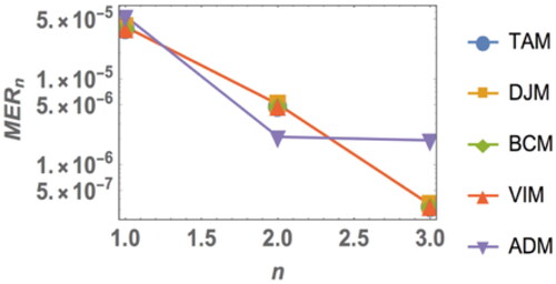
Also, Table 1 shows the${\mathrm{ }\mathit{MER}}_n$ values obtained by TAM, DJM, BCM, VIM and ADM. It can be seen the obtained results are better than ADM (less errors).

Table 1. The${\mathrm{ }\mathit{MER}}_n$ values obtained by TAM, DJM, BCM, VIM and ADM, when $\alpha =0.3,$ L = 4 and t = 0.01.

ni	TAM	DJM	BCM	VIM	ADM
n1	$0.00004070718566899501$	$0.00004070718566900195$	$0.00004070718566900195$	$0.00004070718566900195$	$0.00005410882040962091$
n2	$5.089192788396146\times {10}^{-6}$	$5.089192788378799\times {10}^{-6}$	$5.089192788378799\times {10}^{-6}$	$5.08919278837533\times {10}^{-6}$	$2.1170418793068858\times {10}^{-6}$
n3	$3.410195092909407\times {10}^{-7}$	$3.410195092840018\times {10}^{-7}$	$3.410195092840018\times {10}^{-7}$	$3.41019509308288\times {10}^{-7}$	$1.929269030835451\times {10}^{-6}$

Also, Figures 2–4 show the${\mathrm{ }\mathit{MER}}_n$ values that we get by using different values of α, L and t.

Figure 2. The${\mathrm{ }\mathit{MER}}_n$ values obtained by proposed methods for different values of$\mathrm{ }\alpha ,$ when L = 4 and t = 0.01.

Figure 3. The${\mathrm{ }\mathit{MER}}_n$ values obtained by proposed methods for different values of$\mathrm{ }L,$ when$\mathrm{ }\alpha =0.3\mathrm{ }$ and t = 0.01.

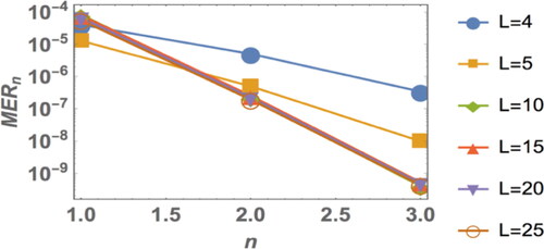
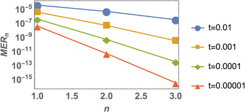
Figure 4. The${\mathrm{ }\mathit{MER}}_n$ values obtained by proposed methods for different values of $t,$ when$\mathrm{ }\alpha =0.3$ and L = 4.

In Figure 2, we fixed the length (L = 4) and the time (t = 0.01) and we used different values for eigenvalue (α = 0.3, 2, 4, 6, 8, 10), depending on previous studies (Bakhtiari et al., 2018; Peletier & Rottschäfer, 2004). We found that the by increasing the value of α, the ${\mathit{MER}}_n$ errors start increasing.

In Figure 3, we fixed the values eigenvalue (α = 0.3) and the time (t = 0.01) and we compared among different value of length (L = 4, 5, 10, 15, 20, 25), as chosen in (Bakhtiari et al., 2018; Peletier & Rottschäfer, 2004). When we increase the value of L, the accuracy increased, and we realized the accuracy almost same when L = 10, 15, 20, 25.

In Figure 4, using different values of the time (t = 0.01, 0.001, 0.0001 and 0.00001), we found that the${\mathrm{ }\mathit{MER}}_n$ decreased whenever the time decreased, and hence the accuracy increased.

The first three iterative methods DJM, TAM and BCM are distinct from other methods as they have many advantages that do not require the conditions of restriction in their implementation and do not require additional calculations for nonlinear problems such as calculating the Adomian polynomials to handle the nonlinear terms in the ADM and calculate the Lagrange multiplier as in the VIM. Moreover, comparing with numerical methods, the iterative methods there is no need to use any type of truncation errors or discretization the domain nor round-off errors.

By making the comparison between the iterative methods with each other, we found that the implementation of the BCM is easier and takes less time compared to the other iterative methods. That is because it adopts the direct technique in the solution during the calculation of the iterations of the desired problem. Also, when applied the TAM, we found in each step a new problem should be solved like a new equation with its conditions, and hence it more effective and time-consuming. On the other hand, the DJM needs more time in terms of calculating the difference for the sum of the iterations. Also, when applying the other two methods the VIM and ADM, we found they require additional calculations and time-consuming such as Adomian polynomials to handle the nonlinear terms in the ADM and calculate Lagrange multiplier as in the VIM and for solving a nonlinear case, the terms of the sequence become complex after several iterations. However, the difficulties of calculating Lagrange multiplier are simplified by using Laplace transform (Anjum & He, 2019) Furthermore, the solution process in three methods BCM, TAM and DJM are derivative-free which are different from VIM.

However, some disadvantages arise by implementing these proposed iterative methods to solve the S-HE. That is related to increasing or decreasing the values of the parameters upon that the problem is under consideration. It was found that this affects the convergence of the solution by using these methods. In other words, by increasing the value of α, the error increases; and hence the accuracy of the method decreases. Moreover, changing the values of the length (L) also affect by convergence; that is, by decreasing and increasing the value of L, the error and accuracy start increasing and decreasing, respectively. One more disadvantage is when the values of time (t) that used for the S-HE increase, the calculated error increases and the proposed iterative methods become less accurate, as shown in Figures 2–4. Finally, increasing the iterations of the proposed became more time-consuming.

7. Conclusion

In this paper, we introduced and applied five iterative methods to solve the 1 D S-HE. We described five iterative methods: DJM, TAM, BCM, ADM, and VIM. The three methods DJM, TAM and BCM can be used without restriction conditions for nonlinear problems unlike VIM and ADM; where they required additional calculations such as Adomian polynomials to handle the nonlinear terms in the ADM and calculate Lagrange multiplier as in the VIM which required more time during the calculation process. It can be concluded, that the ${\mathit{MER}}_n$ starts decreasing by increasing the iterations. Furthermore, the suggested methods: DJM, TAM, BCM, and VIM converge faster, and the results are very accurate and more reliable compared with the ADM.

Acknowledgments

The author would like to thank the anonymous referees, the Managing Editor and Editor in Chief for their valuable suggestions.

Disclosure statement

No potential conflict of interest was reported by the authors.

References

- Abdul Nabi, A. J., & Al-Jawary, M. A. (2018). Analytical and numerical solutions for the linear and nonlinear 1D, 2D and 3D telegraph equations. Journal of Advanced Research in Dynamical & Control Systems, 10(10) (Special Issue), 2090–2105.
- Adomian, G. (1994). Solving frontier problems of physics: The decomposition method. Boston: Klumer.
- Adomian, G. (2014). Nonlinear stochastic operator equations. Academic Press INC (LONDON) LTD.
- Adomian, G., & Rach, R. (1993). Analytic solution of nonlinear boundary-value problems in several dimensions by decomposition. Journal of Mathematical Analysis and Applications, 174(1), 118–137. doi:10.1006/jmaa.1993.1105
- Akbarzade, M., & Langari, J. (2011). Application of variational iteration method to partial differential equation systems. International Journal of Mathematical Analysis, 5(18), 863–870.
- Akyildiz, F. T., Siginer, D. A., Vajravelu, K., & Van Gorder, R. A. (2010). Analytical and numerical results for the Swift–Hohenberg equation. Applied Mathematics and Computation, 216(1), 221–226. doi:10.1016/j.amc.2010.01.041
- Al-Jawary, M. A. (2016). An efficient iterative method for solving the Fokker–Planck equation. Results in Physics, 6, 985–991. doi:10.1016/j.rinp.2016.11.018
- Al-Jawary, M. A. (2017). A semi-analytical iterative method for solving nonlinear thin film flow problems. Chaos, Solitons & Fractals, 99, 52–56. doi:10.1016/j.chaos.2017.03.045
- Al-Jawary, M. A., & Raham, R. K. (2017). A semi-analytical iterative technique for solving chemistry problems. Journal of King Saud University - Science, 29(3), 320–332. doi:10.1016/j.jksus.2016.08.002
- Al-Jawary, M. A., Adwan, M. I., & Radhi, G. H. (2020). Three iterative methods for solving second order nonlinear ODEs arising in physics. Journal of King Saud University-Science, 32(1), 312–323.
- Al-Jawary, M. A., Azeez, M. M., & Radhi, G. H. (2018). Analytical and numerical solutions for the nonlinear Burgers and advection–diffusion equations by using a semi-analytical iterative method. Computers & Mathematics with Applications, 76(1), 155–171. doi:10.1016/j.camwa.2018.04.010
- Al-Jawary, M. A., Radhi, G. H., & Ravnik, J. (2017). Semi-analytical method for solving Fokker-Planck’s equations. Journal of the Association of Arab Universities for Basic and Applied Sciences, 24(1), 254–262. doi:10.1016/j.jaubas.2017.07.001
- Al-Jawary, M. A., Radhi, G. H., & Ravnik, J. (2018). Daftardar-Jafari method for solving nonlinear thin film flow problem. Arab Journal of Basic and Applied Sciences, 25(1), 20–27. doi:10.1080/25765299.2018.1449345
- Anjum, N., & He, J.-H. (2019). Laplace transform: Making the variational iteration method easier. Applied Mathematics Letters, 92, 134–138. doi:10.1016/j.aml.2019.01.016
- Ateeah, A. K. (2017). Approximate solution for fuzzy differential algebraic equations of fractional order using Adomian decomposition method. Ibn AL-Haitham Journal for Pure and Applied Science, 30(2), 202–213.
- Bakhtiari, P., Abbasbandy, S., & Van Gorder, R. A. (2018). Reproducing kernel method for the numerical solution of the 1D Swift–Hohenberg equation. Applied Mathematics and Computation, 339, 132–143. doi:10.1016/j.amc.2018.07.006
- Ban, T., & Cui, R.-Q. (2018). He’s homotopy perturbation method for solving time fractional Swift-Hohenberg equations. Thermal Science, 22(4), 1601–1605. doi:10.2298/TSCI1804601B
- Bhalekar, S., & Daftardar-Gejji, V. (2008). New iterative method: Application to partial differential equations. Applied Mathematics and Computation, 203(2), 778–783. doi:10.1016/j.amc.2008.05.071
- Chossat, P., & Faye, G. (2015). Pattern formation for the Swift-Hohenberg equation on the hyperbolic plane. Journal of Dynamics and Differential Equations, 27(3-4), 485–531. doi:10.1007/s10884-013-9308-3
- Daftardar-Gejji, V., & Bhalekar, S. (2009). Solving nonlinear functional equation using Banach contraction principle. Far East Journal of Applied Mathematics, 34(3), 303–314.
- Daftardar-Gejji, V., & Bhalekar, S. (2010). Solving fractional boundary value problems with Dirichlet boundary conditions using a new iterative method. Computers & Mathematics with Applications, 59(5), 1801–1809. doi:10.1016/j.camwa.2009.08.018
- Daftardar-Gejji, V., & Jafari, H. (2006). An iterative method for solving nonlinear functional equations. Journal of Mathematical Analysis and Applications, 316(2), 753–763. doi:10.1016/j.jmaa.2005.05.009
- Deng, S., & Li, X. (2012). Generalized homoclinic solutions for the Swift–Hohenberg equation. Journal of Mathematical Analysis and Applications, 390(1), 15–26. doi:10.1016/j.jmaa.2011.11.074
- Fonseca, F. (2017). The Solitary Wave Solution of the Swift-Hohenberg equation using He’s semi inverse method. International Mathematical Forum, 12(15), 737–745. doi:10.12988/imf.2017.7758
- Haragus, M., & Scheel, A. (2007). Interfaces between rolls in the Swift-Hohenberg equation. International Journal of Dynamical Systems and Differential Equations, 1(2), 89. doi:10.1504/IJDSDE.2007.016510
- He, J. H. (1999). Variational iteration method-a kind of non-linear analytical technique: Some examples. International Journal of Non-Linear Mechanics, 34(4), 699–708. doi:10.1016/S0020-7462(98)00048-1
- He, J. H. (2007). Variational iteration method—some recent results and new interpretations. Journal of Computational and Applied Mathematics, 207(1), 3–17. doi:10.1016/j.cam.2006.07.009
- He, J. H. (2019a). A modified Li-He’s variational principle for plasma. International Journal of Numerical Methods for Heat and Fluid Flow. doi:10.1108/HFF-06-2019-0523
- He, J. H. (2019b). Lagrange crisis and generalized variational principle for 3D unsteady flow. International Journal of Numerical Methods for Heat & Fluid Flow. doi:10.1108/HFF-07-2019-0577
- He, J. H., & Sun, C. (2019). A variational principle for a thin film equation. Journal of Mathematical Chemistry, 57(9), 2075–2081. doi:10.1007/s10910-019-01063-8
- Kubstrup, C., Herrero, H., & Pérez-García, C. (1996). Fronts between hexagons and squares in a generalized Swift-Hohenberg equation. Physical Review E, 54(2), 1560–1569. doi:10.1103/PhysRevE.54.1560
- Kudryashov, N. A., & Ryabov, P. N. (2016). Analytical and numerical solutions of the generalized dispersive Swift–Hohenberg equation. Applied Mathematics and Computation, 286, 171–177. doi:10.1016/j.amc.2016.04.024
- Mitlif, R. J. (2014). New iterative method for solving nonlinear equations. Baghdad Science Journal, 11(4), 1649–1654. . doi:10.21123/bsj.11.4.1649-1654
- Odibat, Z. M. (2010). A study on the convergence of variational iteration method. Mathematical and Computer Modelling, 51(9-10), 1181–1192. doi:10.1016/j.mcm.2009.12.034
- Peletier, L. A., & Rottschäfer, V. (2004). Pattern selection of solutions of the Swift–Hohenberg equation. Physica D: Nonlinear Phenomena, 194(1-2), 95–126. doi:10.1016/j.physd.2004.01.043
- Peletier, L. A., & Williams, J. F. (2007). Some canonical bifurcations in the Swift–Hohenberg equation. SIAM Journal on Applied Dynamical Systems, 6(1), 208–235. doi:10.1137/050647232
- Pérez-Moreno, S. S., Chavarría, S. R., & Chavarría, G. R. (2014). Numerical solution of the Swift–Hohenberg equation. In: Klapp J., Medina A. (eds) Experimental and computational fluid mechanics (pp. 409–416). Cham: Springer.
- Razzaq, E. A. L. A., & Yassein, S. M. (2017). Analytic solutions for integro-differential inequalities using modified Adomian decomposition method. Ibn AL-Haitham Journal for Pure and Applied Science, 30(1), 177–191.
- Sahib, A. A. A., & Hasan, S. Q. (2014). Convergence of the generalized homotopy perturbation method for solving fractional order integro-differential equations. Baghdad Science Journal, 11(4), 1637–1648. doi:10.21123/bsj.11.4.1637-1648
- Swift, J., & Hohenberg, P. C. (1977). Hydrodynamic fluctuations at the convective instability. Physical Review A, 15(1), 319–328. doi:10.1103/PhysRevA.15.319
- Tao, Y., & Zhang, J. (2002). A shooting method for the Swift-Hohenberg equation. Applied Mathematics-A Journal of Chinese Universities, 17(4), 391–403. doi:10.1007/s11766-996-0003-6
- Temimi, H., & Ansari, A. R. (2011a). A semi-analytical iterative technique for solving nonlinear problems. Computers & Mathematics with Applications, 61(2), 203–210. doi:10.1016/j.camwa.2010.10.042
- Temimi, H., & Ansari, A. R. (2011b). A new iterative technique for solving nonlinear second order multi-point boundary value problems. Applied Mathematics and Computation, 218(4), 1457–1466. doi:10.1016/j.amc.2011.06.029
- Temimi, H., & Ansari, A. R. (2015). A computational iterative method for solving nonlinear ordinary differential equations. LMS Journal of Computation and Mathematics, 18(1), 730–753. doi:10.1112/S1461157015000285
- Wang, H., & Yanti, L. (2011). An efficient numerical method for the quintic complex Swift-Hohenberg equation. Numerical Mathematics: Theory, Methods and Applications, 4(2), 237–254. doi:10.4208/nmtma.2011.42s.7
- Wazwaz, A. M. (2000). A new algorithm for calculating Adomian polynomials for nonlinear operators. Applied Mathematics and Computation, 111(1), 33–51. doi:10.1016/S0096-3003(99)00063-6
- Yin, X.-B., Kumar, S., & Kumar, D. (2015). A modified homotopy analysis method for solution of fractional wave equations. Advances in Mechanical Engineering, 7(12), 168781401562033. doi:10.1177/1687814015620330
- Zhu, Y., Chang, Q., & Wu, S. (2005). A new algorithm for calculating Adomian polynomials. Applied Mathematics and Computation, 169(1), 402–416. doi:10.1016/j.amc.2004.09.082