Stable wave solutions to the Landau-Ginzburg-Higgs equation and the modified equal width wave equation using the IBSEF method

Abstract

The Landau-Ginzburg-Higgs equation and the modified equal width wave equation (MEWE) underscore to describe superconductivity and unidirectional wave propagation in nonlinear media with dispersion systems. In the present study, the improved Bernoulli sub-equation function method (IBSEFM) has been introduced to accomplish applicable soliton solutions to the above stated wave equations. We ascertain adequate soliton solutions, videlicet the combination of hyperbolic function, exponential function etc. and speculate the physical significance of the obtained solutions for the definite values of the included parameters through depicting graphs and interpreted the physical phenomena. It is shown that the IBSEFM is powerful, suitable, direct and provide general wave solutions to NLEEs in mathematical physics.

Keywords:

• Improved Bernoulli sub-equation function method
• Landau-Ginzburg-Higgs equation
• the modified equal width wave equation (MEWE)

1. Introduction

Most of the real-world phenomena can be modeled by class of integrable nonlinear partial differential equations. The analysis of exact and approximate solutions of nonlinear partial differential equations get a very important role in various branches of mathematical-physical sciences, such as plasma physics, fluid mechanics, biology, optical fibers, chemical physics, biophysics, solid-state physics, signal processing, mechanical engineering, system identification, electric control theory and geochemistry and so on. Recently, a number of powerful techniques have been developed to extract exact and explicit solutions of nonlinear physical models with the help of computer algebra, like Maple, Matlab and Mathematica. These include, the differential transform method (Yang, Tenreiro Machado, & Srivastava, 2016), the modified simple equation method and its various extensions (Arnous et al., 2017), the Hirto’s bilinear method (Mirza & Hassan, 2017), the sine-cosine method (Mirzazadeh et al., 2015), the tanh-function expansion and its various modifications (Zdravković, Kavitha, Satarić, Zeković, & Petrović, 2012), the F-expansion method (Akbar & Ali, 2017), the Exp-function method (Zhang, Li, & Zhang, 2016), the modified simple equation method (Khan & Akbar, 2013), the modified exponential function method (Abdelrahman, Zahran, & Khater, 2015), the $(G\mathrm{\prime }/G)$-expansion method (Akbar, Ali, & Roy, 2018; Chen & Li, 2012; Manafian, Lakestani, & Bekir, 2016), the rational $(G\mathrm{\prime }/G)$-expansion method (Islam, Akbar, & Azad, 2018), the extended trial equation method (Mohyud-Din & Irshad, 2017), the improved $\text{tan}\left(\varphi (\xi )\right)$-expansion method (Mohyud-Din, Irshad, Ahmed, & Khan, 2017), the first integral method (Ekici et al., 2016), the homogeneous balance method (Senthilvelan, 2001), the homotopy analysis method (Noor, Haq, Abbasbandy, & Hashim, 2016), the mean Monte Carlo finite difference method (Mohammed, Ibrahim, Siri, & Noor, 2019), the fractional Riccati method and fractional double function method (Wang, Lu, Dai, & Chen, 2020; Wu, Yu, & Wang, 2020), the projective Riccati equation method (Dai, Fan, & Zhang, 2019), the Taylor series method (He, Shen, Ji, & He, 2020; He et al., 2020), the variational iteration method (He, 2000, 2011; He & Jin, 2020; He & Latifizadeh, 2020), the modified variational iteration algorithms (Ahmad, Khan, & Cesarano, 2019; Ahmad, Khan, & Yao, 2020; Ahmad, Seadawy, & Khan, 2020a, 2020b; Ahmad, Seadawy, Khan, & Thounthong, 2020; Ahmad & Khan, 2019a, 2019b), the homotopy perturbation method (He, 2019a, 2019b; Yu, He, & Garcıa, 2019), the generalized Bernoulli sub-ODE method (Özpinar, Baskonus & Bulut, 2015; Zheng, 2012) and others (Chen, Lin, & Wang, 2019; Dai, Wang, Fan, & Zhang, 2020).

In this article, we analyze the (1 + 1)-dimensional Landau-Ginzburg-Higgs equation (Bekir & Unsal, 2013; Cevikel, Aksoy, Guner, & Bekir, 2013; Hu, Deng, Han, & Fa, 2009; Iftikhar, Ghafoor, Zubair, Firdous, & Mohyud-Din, 2013; Irshad et al., 2017): (1) $$u_{tt}-u_{xx}-m^{2}u+n^2{u}^3=0,$$(1) and the solitary wave equation of the modified equal width wave (MEWE) (Ali, Soliman, & Raslan, 2007; Evans & Raslan, 2005a, 2005b; Lu, Seadawy, & Ali, 2018; Rab & Akhter, 2013; Raslan, 2006, 2008; Raslan, Khalid, & Shallal, 2017) equation: (2) $$u_t+u^2{u}_x-u_{\mathit{xxt}}=0.$$(2)

The Landau-Ginzburg-Higgs equation (1)(1) $$u_{tt}-u_{xx}-m^{2}u+n^2{u}^3=0,$$(1) investigated through some methods, videlicet by the multi-symplectic Runge-Kutta method (Hu et al., 2009), the $(G\mathrm{\prime }/G, 1/G)$-expansion method (Iftikhar et al., 2013), the sine-cosine method and the extended tanh method (Cevikel et al., 2013), the first integral method (Bekir & Unsal, 2013), the new modified simple method (Irshad et al., 2017). And the solitary wave equation MEWE examined via some analytical schemes, as for instance the first integral method (Raslan, 2008), the sine-function method (Rab & Akhter, 2013), the extended simple equation method and the exp$(-\phi (\xi ))$ expansion method (Lu et al., 2018), the tanh function method (Evans & Raslan, 2005a), the collocation method using quadratic B-spline (Evans & Raslan, 2005b), the collocation method using cubic B-spline (Raslan, 2006), the modified extended tanh method (Raslan et al., 2017), Cosine-function method (Ali et al., 2007) etc. To our foremost understanding, the above stated equations have not been examined through the improved Bernoulli sub-equation function method (IBSEFM) (Aksan, Bulut, & Kayhan, 2017; Baskonus, Koc, & Bulut, 2016a, 2016b; Baskonus & Bulut, 2015; Dusunceli, 2018, 2019; Yokus, Baskonus, Sulaiman, & Bulut, 2018). Therefore, motivated by the above studies, the aim of this research is to establish adequate stable general and broad-ranging soliton solutions associated with free parameters to the earlier stated equations through the IBSEF method with the combination of hyperbolic function, exponential function etc. Setting definite values of the free parameters some typical solutions are originated and some fresh solutions are established. It is worth mentioning that some well-known solutions explicitly, the bell-shape soliton, singular bell-shape soliton, kink, periodic waves have emerged from the broad-ranging general solution.

The residue of this article is comprised in several sections: In second part, we identify the steps of IBSEFM, and then in the third part the IBSEFM method is put in use to the earlier equations. The fourth part contains the results and discussions and in final part conclusion is given.

2. Material and method

The improved Bernoulli sub-equation function method (IBSEFM) was developed from the Bernoulli sub-equation function method (Zheng, 2011) whose courses of action are as follows:

Step I: We consider subsequent nonlinear evolution equation: (3) $$P\left(u,u_x,u_y,u_z,u_t,u_{tt},u_{tx},u_{xx},u_{yy},u_{zz},\dots \right)=0,$$(3) and the wave variable (4) $$u\left(x,y,z,t\right)=U\left(\eta \right), \eta =l_{1}x+l_{2}y+\omega t.$$(4)

The wave transformation (4) modifies the Equation (3)(3) $$P\left(u,u_x,u_y,u_z,u_t,u_{tt},u_{tx},u_{xx},u_{yy},u_{zz},\dots \right)=0,$$(3) into a nonlinear ordinary differential equation of the following (5) $$Q\left(U,U^{\mathrm{\prime }},U^{\text{″}},U^{\text{‴}},\dots \right)=0.$$(5)

Step II: As per the improved Bernoulli sub-equation function method, the solution is taken in the succeeding form: (6) $$U\left(\eta \right)=\frac{\sum _{i=0}^q{a}_i{G}^i}{\sum _{j=0}^p{b}_j{G}^j}=\frac{a_0+a_{1}G+a_2{G}^2+ \dots +a_q{G}^q}{b_0+b_{1}G+b_2{G}^2+b_3{G}^3+ \dots +b_p{G}^p},$$(6) where $G=G(\eta )$ is the solution of the improved Bernoulli equation (7) $$G^{\mathrm{\prime }}=\sigma G+d{G}^M, \sigma \ne 0,d\ne 0,M\in \mathbb{R}-\{0,1,2\}.$$(7)

The value of the unknown parameters $p$ and $q$ can be found out by figuring out the homogeneous balance of the highest order linear term with the nonlinear term of the highest order. This technique gives the values of $q$ and $p.$

Inserting the solution (6) into the Equation (5)(5) $$Q\left(U,U^{\mathrm{\prime }},U^{\text{″}},U^{\text{‴}},\dots \right)=0.$$(5) and making use of the Equation (7)(7) $$G^{\mathrm{\prime }}=\sigma G+d{G}^M, \sigma \ne 0,d\ne 0,M\in \mathbb{R}-\{0,1,2\}.$$(7) , it provides us a polynomial equation $\mathrm{\Omega }\left(G\right)$ of $G:$ (8) $$\mathrm{\Omega }\left(G\right)={\rho }_s{G}^s+ \dots +{\rho }_{1}G+{\rho }_0=0.$$(8)

Step III. Equalizing the coefficients of $\mathrm{\Omega }(\mathrm{G})$ to zero yields a system of equations: (9) $${\rho }_k=0, k=0, \dots ,s.$$(9)

Solving the system, we obtain the definite the values of $a_0,\dots ,a_q$ and $b_0,b_1,\dots ,b_p.$

Step IV. The solutions of the nonlinear Bernoulli differential equation (7)(7) $$G^{\mathrm{\prime }}=\sigma G+d{G}^M, \sigma \ne 0,d\ne 0,M\in \mathbb{R}-\{0,1,2\}.$$(7) depend on the values of $\sigma$ and $d.$ The two types of solutions of the improved Bernoulli’s equation are as following: (10) $$G\left(\eta \right)={\left[-\frac{d}{\sigma }+\frac{\tau }{e^{\left(\sigma \right(M-1)\eta }}\right]}^{\frac{1}{1-M}}, \sigma \ne d,$$(10) (11) $$G\left(\eta \right)={\left[\frac{\left(\tau -1\right)+\left(\tau +1\right)\tanh \left(\frac{\sigma \left(1-M\right)\eta }{2}\right)}{1-\tanh \left(\frac{\sigma \left(1-M\right)\eta }{2}\right)}\right]}^{\frac{1}{1-M}},\sigma =d, \tau \in \mathbb{R}.$$(11)

Using a whole distinction system for polynomial of $G,$ we analyse Equation (9)(9) $${\rho }_k=0, k=0, \dots ,s.$$(9) by using of Maple and pertain the exact solutions to Equation (5)(5) $$Q\left(U,U^{\mathrm{\prime }},U^{\text{″}},U^{\text{‴}},\dots \right)=0.$$(5) .

3. Formulation of the solutions

The purpose of this section is to obtain stable broad-ranging general solution to the Landau-Ginzburg-Higgs equation and MEWE equation by using the IBSEF method from which some existing solutions in the literature and some fresh closed form wave solutions can be extracted.

3.1. The Landau-Ginzburg-Higgs equation

In this sub-section, application of the improved Bernoulli sub-equation function method to Landau-Ginzburg-Higgs equation is presented. Using the wave transformation (12) $$u\left(x,t\right)=U\left(\eta \right), \eta =x-c t,$$(12)

Equation (1)(1) $$u_{tt}-u_{xx}-m^{2}u+n^2{u}^3=0,$$(1) , is converted to a NODE as follows: (13) $$\left(c^2-1\right)U^{\text{″}}-m^{2}U+n^2{U}^3=0.$$(13)

The homogeneous balancing principle between $U\mathrm{\prime }\mathrm{\prime }$ and $U^3,$ yields a relation for $p,$ $q$ and $M$ as: $$p+M=q+1.$$

For the free parameters, choosing $M=3,$ $p=1$ gives $q=3.$ Thus, the provisional solution to Equation (13)(13) $$\left(c^2-1\right)U^{\text{″}}-m^{2}U+n^2{U}^3=0.$$(13) takes the following form (14) $$U\left(\eta \right)=\frac{a_0+a_{1}G\left(\eta \right)+a_2{G}^2\left(\eta \right)+a_3{G}^3\left(\eta \right)}{b_0+b_{1}G\left(\eta \right)},$$(14) where $G$ is the solution of the improved Bernoulli equation (7)(7) $$G^{\mathrm{\prime }}=\sigma G+d{G}^M, \sigma \ne 0,d\ne 0,M\in \mathbb{R}-\{0,1,2\}.$$(7) .

Embedding solution (14), together with Equation (7)(7) $$G^{\mathrm{\prime }}=\sigma G+d{G}^M, \sigma \ne 0,d\ne 0,M\in \mathbb{R}-\{0,1,2\}.$$(7) into Equation (13)(13) $$\left(c^2-1\right)U^{\text{″}}-m^{2}U+n^2{U}^3=0.$$(13) , it yields a polynomial in $G$ and setting each coefficient of this polynomial to zero yields a system of over-determined equations. Solving the system of the algebraic equations, we attain the subsequent set of solutions of the parameters:

Case 1: For $\sigma \ne d,$ the scores of the arguments are found in the following:

Set 1. (15) $$c=\pm \frac{\sqrt{-2m^2+4{\sigma }^2}}{2\sigma }, a_0=\frac{a_2\sigma }{2d} a_1=\frac{b_{1}m}{n}, a_3=\frac{2b_{1}md}{n\sigma }, b_0=\frac{a_{2}n\sigma }{2md},$$(15)

Set 2. (16) $$c=\pm \frac{\sqrt{-2m^2+4{\sigma }^2}}{2\sigma }, a_0=\frac{a_2\sigma }{2d} a_1=-\frac{b_{1}m}{n}, a_3=-\frac{2b_{1}md}{n\sigma }, b_0=-\frac{a_{2}n\sigma }{2md}$$(16)

By means of the values of the parameters congregated in (15) into solution (14), we attain (17) $$u\left(x,t\right)=-\frac{m(d{\mathit{e}}^{2x\sigma -t\sqrt{-2m^2+4{\sigma }^2}}+\sigma \tau )}{n(d{\mathit{e}}^{2x\sigma -t\sqrt{-2m^2+4{\sigma }^2}}-\sigma \tau )}$$(17)

After simplification, solution (17) can be written in the form (18) $$u_1\left(x,t\right)=-\frac{m}{n} \frac{\left(d+\sigma \tau \right)\cosh \psi +\left(d-\sigma \tau \right)\sinh \psi }{\left(d-\sigma \tau \right)\cosh \psi +\left(d+\sigma \tau \right)\text{ sinh }\psi },$$(18) where $\psi =(2x\sigma -t\sqrt{-2m^2+4{\sigma }^2})/2.$

When $d=\sigma \tau ,$ substituting $\psi =\psi =(2x\sigma -t\sqrt{-2m^2+4{\sigma }^2})/2,$ we attain (19) $$u_{1_{11}}\left(x,t\right)=-\frac{m}{n}\coth \frac{1}{2}\left(2x\sigma -t\sqrt{-2m^2+4{\sigma }^2}\right),$$(19)

On the other hand, when $d=-\sigma \tau ,$ we accomplish the subsequent solution (20) $$u_{1_{12}}\left(x,t\right)=-\frac{m}{n}\tanh \frac{1}{2}\left(2x\sigma -t\sqrt{-2m^2+4{\sigma }^2}\right),$$(20)

Case 2: For $\sigma \ne d,$ we attain the solution as follows: (21) $$u_2\left(x,t\right)=\frac{m}{n}\left\{\frac{\left(-1-\tau \right)\mathrm{cosh }\psi + \left(-1+\tau \right) \sinh \psi }{\left(1-\tau \right)\mathrm{cosh }\psi +\left(1+\tau \right) \sinh \psi }\right\}.$$(21)

When $\tau =1$ and using $\psi =(2x\sigma -t\sqrt{-2m^2+4{\sigma }^2})/2,$ we secure (22) $$u_{2_{11}}\left(x,t\right)=-\frac{m}{n}\coth \frac{1}{2}\left(2x\sigma -t\sqrt{-2m^2+4{\sigma }^2}\right).$$(22)

Again if $\tau =-1$ and putting $=2x\sigma -t\sqrt{-2m^2+4{\sigma }^2},$ we accomplish (23) $$u_{2_{12}}\left(x,t\right)=-\frac{m}{n}\tanh \frac{1}{2}\left(2x\sigma -t\sqrt{-2m^2+4{\sigma }^2}\right).$$(23)

Similarly the other choice of the values of $d$ and $\tau$ provide many other closed form wave solutions to the Landau-Ginzburg-Higgs equation but for conciseness, the other solutions have not been documented here.

For the values of the parameters assembled in (16), we will attain analogous structured solutions attained for values arranged in (15). But, to avoid deception, the solutions have not been written here.

3.2. The modified equal width wave equation (MEWE)

In this sub-section, we will bring to bear the improved Bernoulli sub-equation function method to extract exact wave solutions to the modified equal width wave equation (MEWE). Using the subsequent wave transformation (24) $$u\left(x,t\right)=U\left(\eta \right), \eta =x-ct,$$(24) the MEWE modifies into the under mentioned NODE: (25) $$3c{U}^{\text{″}}+U^3-3cU=0.$$(25)

The balancing principle between $U\mathrm{\prime }\mathrm{\prime }$ and $U^3,$ we obtain the relation for $p,$ $q$ and $M$ as: $$p+M=q+1.$$

For simplicity, choosing the free parameters $M=3,$ $p=1$ gives $q=3.$ Thus, the provisional solution to Equation (25)(25) $$3c{U}^{\text{″}}+U^3-3cU=0.$$(25) takes the following form: (26) $$U\left(\eta \right)=\frac{a_0+a_{1}G\left(\eta \right)+a_2{G}^2\left(\eta \right)+a_3{G}^3\left(\eta \right)}{b_0+b_{1}G\left(\eta \right)},$$(26) where $G$ is the solution to the improved Bernoulli equation.

Inserting solution (26), together with Equation (7)(7) $$G^{\mathrm{\prime }}=\sigma G+d{G}^M, \sigma \ne 0,d\ne 0,M\in \mathbb{R}-\{0,1,2\}.$$(7) into Equation (25)(25) $$3c{U}^{\text{″}}+U^3-3cU=0.$$(25) , it yields a polynomial in $G$ and hence a system of algebraic equations. Unraveling the system of the algebraic equations, we attain the subsequent set of solutions of the parameters:

For $\sigma \ne d,$ we derive the score of the parameters provided in the next:

Set 1: (27) $$c=-\frac{a_3^2}{24d^2{b}_1^2}, a_0=0, a_1=\pm \frac{a_3\sqrt{-2}}{4d}, a_2=0, b_0=0, \sigma =\pm \sqrt{\frac{-1}{2}}$$(27)

Set 2: (28) $$c=-\frac{a_3^2}{24d^2{b}_1^2},a_0=\pm \frac{a_3{b}_0\sqrt{-2}}{4b_{1}d},a_1=\pm \frac{a_3\sqrt{-2}}{4d},a_2=\frac{a_3{b}_0}{b_1},\sigma =\pm \sqrt{\frac{-1}{2}}$$(28)

Case 1: When $d\ne \sigma =\pm \sqrt{\frac{-1}{2}},$ substituting the values of the parameters arranged in (27) into solution (26), we derive (29) $$u_3\left(x,t\right)=\frac{a_3\left(\left(-id+\frac{\tau }{\sqrt{2}}\right)\cosh \xi +\left(-id-\frac{\tau }{\sqrt{2}}\right)\sinh \xi \right)}{4d{b}_1\left(\left(\frac{d}{\sqrt{2}}-\frac{i\tau }{2}\right)\mathrm{cosh }\xi +\left(\frac{d}{\sqrt{2}}+\frac{i\tau }{2}\right)\sinh \xi \right)},$$(29) where $\xi =\sqrt{-2}\left(x+\frac{t{a}_3^2}{24d^2{b}_1^2}\right)/2.$

If $d=\sqrt{-\frac{1}{2}}\tau ,$ we attain (30) $$u_{3_{11}}\left(x,t\right)=\frac{{-a}_3}{2b_1}\mathrm{ coth}\sqrt{-\frac{1}{2}}\left(x-\frac{t{a}_3^2}{12{\mathrm{\tau }}^2{b}_1^2}\right).$$(30)

Again, if $d=-\sqrt{-\frac{1}{2}}\tau ,$ we attain (31) $$u_{3_{12}}\left(x,t\right)=\frac{-a_3}{2b_1}\mathrm{ tanh}\sqrt{-\frac{1}{2}}\left(x-\frac{t{a}_3^2}{12{\mathrm{\tau }}^2{b}_1^2}\right)$$(31)

Case 2: When $d=\sigma =\pm \sqrt{\frac{-1}{2}},$ substituting the values of the parameters arranged in (27) into solution (26) gives (32) $$u_4(x,t)=\frac{a_3\left(i\left(1+\tau \right)\cosh \xi +\left(-1+\tau \right)\sinh \xi \right)}{2b_1\left(i\left(1+\tau \right)\cosh \xi +\left(-1+\tau \right)\text{sin}\xi \right)}.$$(32)

We attain the solution substituting $\xi =\frac{1}{\sqrt{2}}\left(x-\frac{t{a}_3^2}{12b_1^2}\right)$ and $\tau =1,$ (33) $$u_{4_{11}}\left(x,t\right)=\frac{a_{3}i}{2b_1}\coth \frac{1}{\sqrt{2}}\left(x-\frac{t{a}_3^2}{12b_1^2}\right).$$(33)

If $\tau =-1$ and replacing $\xi =\frac{1}{\sqrt{2}}\left(x-\frac{t{a}_3^2}{12b_1^2}\right),$ we establish the kink solution (34) $$u_{4_{12}}\left(x,t\right)=\frac{a_3}{2{ib}_1}\tanh \frac{\xi }{2}$$(34)

If we use the values of the parameters recorded in (28), likewise, we will gain further solutions homologous to the general solutions (29) and (32). For the sagacity, these solutions have been ignored. It is important to note that the wave solutions (29) and (32) of the modified equal width wave equation (MEWE) are resourceful and were not established in the earlier research. The above solutions might be fruitful to investigate the unidirectional wave propagation in nonlinear media with dispersion relativistic one-particle theory etc.

4. Results and discussion

In this section, the obtained wave solutions have been depicted in the figures and talk over the natures of these wave solutions for various values of the parameters with the aid of symbolic computation software Mathematica.

4.1. Graphical representation of the solution of the Landau-Ginzburg-Higgs equation

In this subsection, we have presented the graphical evolution of the derived results to the Landau-Ginzburg-Higgs equation for diverse values of the parameters. The 3D and 2D graphs of the solutions of the Landau-Ginzburg-Higgs equation are shown at the underneath:

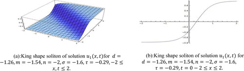
Solution $u_1(x,t)$ represents kink shape wave for the values $d=-1.26,$ $m=-1.54,$ $n=-2,$ $\sigma =-1.6,$ $\tau =-0.29$ within the interval $-2\le x,t\le 2$ and shown in Figure 1. Kink waves are traveling waves which incline or upsurge from one asymptotic state to another. Solution $u_2(x,t)$ is analogous to the figure of solution $u_1(x,t).$ Therefore it is excluded here to the simplicity.

Figure 1. (a): King shape soliton of solution $u_1(x,t)$ for $d=-1.26,m=-1.54,n=-2,\sigma =-1.6,$ $\tau =-0.29, -2\le x,t\le 2.$ (b): King shape soliton of solution $u_1(x,t)$ for $d=-1.26,m=-1.54,n=-2,\sigma =-1.6,$ $\tau =-0.29, t=0-2\le x\le 2.$

Solution $u_{1_{12}}(x,t)$ represents sharp slope bell shape soliton for the values $m=-7,$ $n=1,$ $\sigma =1$ within the intervals $0.1\le t\le 0.2,$ $-1\le x\le 1$ and presented in Figure 2.

Figure 2. (a): Sharp slope bell shape soliton of solution $u_{1_{12}}(x,t)$ for $m=-7,n=1,\sigma =1,-0.1\le t\le 0.2,-1\le x\le 1.$ (b): Sharp slope bell shape soliton of solution $u_{1_{12}}(x,t)$ for $m=-7,n=1,\sigma =1,t=0,-1\le x\le 1.$

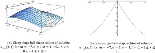
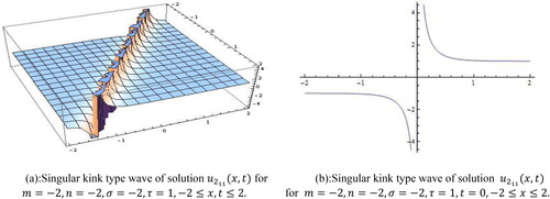
Solution $u_{2_{12}}(x,t)$ also represents the same shape. In order to avoid repetition, the pattern has been ignored. Solution $u_{2_{11}}(x,t)$ represents singular kink shape soliton for the values $d=-2,$ $m=-2,$ $n=-2,$ $\sigma =-2,$ $\tau =1$ within the interval $-2\le x,t\le 2$ and displayed in Figure 3. We attain the same shape for solution ${u_1}_{11}(x, t).$

Figure 3. (a): Singular kink type wave of solution $u_{2_{11}}(x,t)$ for $m=-2,n=-2,\sigma =-2,\tau =1, -2\le x,t\le 2.$ (b): Singular kink type wave of solution $u_{2_{11}}(x,t)$ for $m=-2,n=-2,\sigma =-2,\tau =1, t=0,-2\le x\le 2.$

It is perceive that there are several types such as king shape, singular kink shape, bell shape wave are represented by the solutions to the Landau-Ginzburg-Higgs equation for different values of the parameters.

4.2. Graphical representation of the solution of the MEWE

In this subsection, we have presented the graphical evolution of the derived results to the MEWE equation for different values of the parameters.

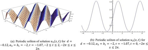
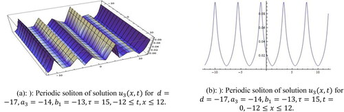
Family $u_3(x,t)$ represents periodic soliton for the values $d=-0.12,$ $a_3=-2,$ $b_1=-2,$ $\tau =-1.07$ within the interval $-2\le t\le 2,$ $-2\pi \le x\le 2\pi$ and demonstrated in Figure 4. We attain the similar shape of the solutions $u_{3_{11}}(x,t)$ and $u_{3_{12}}(x,t).$ To avoid duplicity we escape them.

Figure 4. (a): Periodic soliton of solution $u_3(x,t)$ for $d=-0.12,a_3=b_1=-2,\tau =-1.07, -2\le t\le 2,-2\pi \le x\le 2\pi .$ (b): Periodic soliton of solution $u_3(x,t)$ for $d=-0.12,a_3=b_1=-2,\tau =-1.07, t=0,-2\pi \le x\le 2\pi .$

Family $u_3(x,t)$ signifies periodic soliton for the values $d=-17,$ $a_3=-14,$ $b_1=-13,$ $\tau =15$ within the limit $-12\le t,x\le 12$ and portrayed in Figure 5.

Figure 5. (a): Periodic soliton of solution $u_3(x,t)$ for $d=-17,a_3=-14, b_1=-13,\tau =15, -12\le t,x\le 12.$ (b): Periodic soliton of solution $u_3(x,t)$ for $d=-17,a_3=-14, b_1=-13,\tau =15,t=0, -12\le x\le 12.$

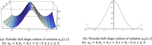
Family $u_4(x,t)$ shows periodic bell shape soliton for the values of $a_3=4,$ $b_1=4,$ $\tau =3$ within the limit $-3\le t,x\le 3$ and interpreted in Figure 6.

Figure 6. (a): Periodic bell shape soliton of solution $u_4(x,t)$ for $a_3=4, b_1=4,\tau =3, -3\le t,x\le 3.$ (b): Periodic bell shape soliton of solution $u_4(x,t)$ for $a_3=4, b_1=4,\tau =3, t=0,-3\le x\le 3.$

Family $u_{4_{11}}(x,t)$ shows singular bell shape soliton for the values $a_3=-2,$ $b_1=-2,$ $\tau =1$ within the limit $-8\le t,x\le 8$ and specified in Figure 7.

Figure 7. (a): singular bell shape soliton of solution $u_{4_{11}}(x,t)$ for $a_3=-2, b_1=-2,\tau =1, -8\le t,x\le 8.$ (b): singular bell shape soliton of solution $u_{4_{11}}(x,t)$ for $a_3=-2, b_1=-2,\tau =1,t=0, -8\le x\le 8.$

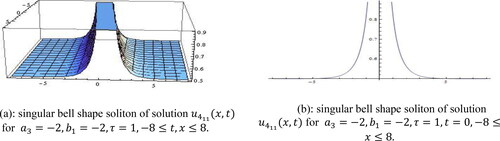
Singular structures (Figures 3 and 7) are another kind of solitary waves that appear with a singularity which are usually infinite discontinuity. Singular solitons can be connected to solitary waves when the position of the center of the solitary wave is imaginary. This solution has spike and therefore it can probably provide an explanation to the formation of Rogue waves (Akbar & Ali, 2016). Periodic traveling waves (Figures 4–6) play a significant role in numerous physical phenomena, including reaction-diffusion-advection systems, impulsive systems, self-reinforcing systems, etc. Mathematical modeling of many intricate physical events, for example chemistry, biology, physics, mathematical physics and several phenomena look like periodic traveling wave solutions (Akbar & Ali, 2016).

5. Conclusions

In this article, the improved Bernoulli sub-equation function method (IBSEFM) has successfully been put in used and established stable general, broad-ranging, typical and fresh soliton solutions to the Landau-Ginzburg-Higgs equation and the modified equal width wave equation (MEWE). We have attained further general and new stable wave solutions which are not reported in the previous literature. The fresh solutions are ascertained as the combination of exponential functions, hyperbolic functions and trigonometric functions associated with several free parameters. The significance of the solutions obtained with free parameters can be important to interpret explain intricate tangible phenomena. The devised algorithm is effective and can be used to unravel other nonlinear evolution equations turn up in mathematical physics and engineering. Thus to test the range of applicability and consistency, the method could be implemented to other kinds of integer and fractional differential systems and this is the concern of further research.

Acknowledgments

The authors would like to express their sincere thanks to the anonymous referees for their valuable comments and suggestions to improve the quality of this article. The authors would also like to acknowledge Md. Rawshan Yeazdani, Department of English, Pabna University of Science and Technology, Bangladesh for his assistance in editing the English language and grammatical errors.

References

- Abdelrahman, A. E., Zahran, E. H. M., & Khater, M.M.A. (2015). The exp (ϕ(ξ))-expansion method and its application for solving nonlinear evolution equations. International Journal of Modern Nonlinear Theory and Application, 4(01), 37–47. doi:10.4236/ijmnta.2015.41004
- Ahmad, H., & Khan, T.A. (2019a). Variational iteration algorithm-I with an auxiliary parameter for the solution of differential equations of motion for simple and damped mass-spring systems. Noise & Vibration Worldwide, 51(1–2), 12–19. doi:10.1177/0957456519889958
- Ahmad, H., & Khan, T. A. (2019b). Variational iteration algorithm-I with an auxiliary parameter for wave-like vibration equations. Journal of Low Frequency Noise, Vibration and Active Control, 38(3–4), 1113–1124. doi:10.1177/1461348418823126
- Ahmad, H., Khan, T. A., & Cesarano, C. (2019). Numerical solutions of coupled Burgers’ equations. Axioms, 8, 119. doi:10.3390/axioms8040119
- Ahmad, H., Khan, T. A., & Yao, S. W. (2020). Numerical solution of second order Painlev´e differential equation. Journal of Mathematics and Computer Science, 21, 150–157. doi:10.22436/jmcs.021.02.06
- Ahmad, H., Seadawy, A. R., & Khan, T. A. (2020a). Numerical solution of Korteweg-de Vries-Burgers equation by the modified variational iteration algorithm-II arising in shallow water waves. Physica Scripta, 95(4), 45210. doi:10.1088/1402-4896/ab6070
- Ahmad, H., Seadawy, A. R., & Khan, T. A. (2020b). Study on numerical solution of dispersive water wave phenomena by using a reliable modification of variational iteration algorithm. Mathematics and Computers in Simulation, 177, 13–23. doi:10.1016/j.matcom.2020.04.005
- Ahmad, H., Seadawy, A. R., Khan, T. A., & Thounthong, P. (2020). Analytic approximate solutions for some nonlinear parabolic dynamical wave equations. Journal of Taibah University for Science, 14(1), 346–358. doi:10.1080/16583655.2020.1741943
- Akbar, M. A., & Ali, N. H. M. (2016). An ansatz for solving nonlinear partial differential equations in mathematical physics. SpringerPlus, 5, 24. doi:10.1186/s40064-015-1652-9
- Akbar, M.A., & Ali, N. H. M. (2017). The improved F-expansion method with Riccati equation and its applications in mathematical physics. Cogent Mathematics, 4(1), 1282577. doi:10.1080/23311835.2017.1282577
- Akbar, M. A., Ali, N. H. M., & Roy, R. (2018). Closed form solutions of two time fractional nonlinear wave equations. Results in Physics, 9, 1031–1039. doi:10.1016/j.rinp.2018.03.059
- Aksan, E. N., Bulut, H., & Kayhan, M. (2017). Some wave simulation properties of the (2 + 1) dimensional breaking solution equation. ITM Web of Conferences, 13, 1014. doi:10.1051/itmconf/20171301014
- Ali, A. H. A., Soliman, A.-M., & Raslan, K. R. (2007). Soliton solution for nonlinear partial differential equations by cosine-function method. Physics Letters A, 368(3–4), 299–304. doi:10.1016/j.physleta.2007.04.017
- Arnous, A. H., Ullah, M. Z., Moshokoa, S. P., Zhou, Q., Triki, H., Mirzazadeh, M., & Biswas, A. (2017). Optical solitons in birefringent fibers with modified simple equation method. Optik - Optik, 130, 996–1003. doi:10.1016/j.ijleo.2016.11.101
- Baskonus, H. M., & Bulut, H. (2015). On the complex structures of Kundu-Eckhaus equation via improved Bernoulli sub-equation function method. Waves in Random and Complex Media, 25(4), 720–728. doi:10.1080/17455030.2015.1080392
- Baskonus, H. M., Koc, D. A., & Bulut, H. (2016a). New travelling wave prototypes to the nonlinear Zakharov-Kuznetsov equation with power law nonlinearity. Nonlinear Science Letters A, 7, 67–76.
- Baskonus, H. M., Koc, D. A., & Bulut, H. (2016b). Dark and new travelling wave solutions to the nonlinear evolution equation. Optik, 127(19), 8043–8055. doi:10.1016/j.ijleo.2016.05.132
- Bekir, A., & Unsal, O. (2013). Exact solutions for a class of nonlinear wave equations by using first integral method. International Journal of Nonlinear Science, 15(2), 99–110.
- Cevikel, A. C., Aksoy, E., Guner, O., & Bekir, A. (2013). Dark-bright soliton solutions for some evolution equations. International Journal of Nonlinear Science, 16(3), 195–202.
- Chen, J., & Li, B. (2012). Multiple (G′/G)-expansion method and its applications to nonlinear evolution equations in mathematical physics. Pramana, 78(3), 375–388. doi:10.1007/s12043-011-0237-6
- Chen, S. J., Lin, J. N., & Wang, Y. Y. (2019). Soliton solutions and their stabilities of three (2 + 1)-dimensional PT-symmetric nonlinear Schrödinger equations with higher-order diffraction and nonlinearities. Optik, 194, 162753. doi:10.1016/j.ijleo.2019.04.099
- Dai, C. Q., Fan, Y., & Zhang, N. (2019). Re-observation on localized waves constructed by variable separation solutions of (1 + 1)-dimensional coupled integrable dispersionless equations via the projective Riccati equation method. Applied Mathematics Letters, 96, 20–26. doi:10.1016/j.aml.2019.04.009
- Dai, C. Q., Wang, Y. Y., Fan, Y., & Zhang, J. F. (2020). Interactions between exotic multi-valued solitons of the (2 + 1)-dimensional Korteweg-de-Vries equation describing shallow water wave. Applied Mathematical Modelling, 80, 506–515. doi:10.1016/j.apm.2019.11.056
- Dusunceli, F. (2018). Solutions for the Drinfeld-Sokolov equation using an IBSEFM method. MSU Journal of Science, 6(1), 505–510. doi:10.18586/msufbd.403217
- Dusunceli, F. (2019). New exponential and complex traveling wave solutions to the konopelchenko- dubrovsky model. Advances in Mathematical Physics, 2019, 1–9. doi:10.1155/2019/7801247
- Ekici, M., Mirzazadeh, M., Eslami, M., Zhou, Q., Moshokoa, S.P., Biswas, A., & Belic, M. (2016). Optical soliton perturbation with fractional-temporal evolution by first integral method with conformable fractional derivatives. Optik - Optik, 127(22), 10659–10669. doi:10.1016/j.ijleo.2016.08.076
- Evans, D. J., & Raslan, K. R. (2005a). The tanh function method for solving some important nonlinear partial differential equation. International Journal of Computer Mathematics, 82(7), 897–905. doi:10.1080/00207160412331336026
- Evans, D. J., & Raslan, K. R. (2005b). Solitary waves for the generalized equal width (GEW) equation. International Journal of Computer Mathematics, 82(4), 445–455. doi:10.1080/0020716042000272539
- He, C. H., Shen, Y., Ji, F. Y., & He, J. H. (2020). Taylor series solution for fractal Bratu-type equation arising in electro-spinning process. Fractals, 28(01), 2050011. doi:10.1142/S0218348X20500115
- He, J. H. (2000). Α review on some new recently developed nonlinear analytical techniques. International Journal of Nonlinear Sciences and Numerical Simulation, 1(1), 51–70. doi:10.1515/IJNSNS.2000.1.1.51
- He, J. H. (2011). A short remark on fractional variational iteration method. Physics Letters A, 375(38), 3362–3364. doi:10.1016/j.physleta.2011.07.033
- He, J. H. (2019a). The simpler, the better: Analytical methods for nonlinear oscillators and fractional oscillators. Journal of Low Frequency Noise, Vibration and Active Control, 38(3–4), 1252–1260. doi:10.1177/1461348419844145
- He, J. H. (2019b). The simplest approach to nonlinear oscillators. Results in Physics, 15, 102546. doi:10.1016/j.rinp.2019.102546
- He, J. H. (2020). Taylor series solution for a third order boundary value problem arising in architectural engineering. Ain Shams Engineering Journal (Journal), 1–4. doi:10.1016/j.asej.2020.01.016
- He, J. H., & Jin, X. (2020). A short review on analytical methods for the capillary oscillator in a nanoscale deformable tube. Mathematical Methods in the Applied Sciences, 2020, 1–8. doi:10.1002/mma.6321
- He, J. H., & Latifizadeh, H. (2020). A general numerical algorithm for nonlinear differential equations by the variational iteration method. International Journal of Numerical Methods for Heat & Fluid Flow, 1–14. doi:10.1108/HFF-01-2020-0029
- Hu, W. P., Deng, Z. C., Han, S. M., & Fa, W. (2009). Multi-symplectic Runge-Kutta methods for Landau Ginzburg-Higgs equation. Applied Mathematics and Mechanics, 30(8), 1027–1034. doi:10.1007/s10483-009-0809-x
- Iftikhar, A., Ghafoor, A., Zubair, T., Firdous, S., & Mohyud-Din, S. T. (2013). (G′/G, 1/G)-expansion method for traveling wave solutions of (2 + 1) dimensional generalized KdV, Sine Gordon and Landau-Ginzburg-Higgs equations. Scientific Research and Essays, 8(28): 1349–1359.
- Irshad, A., Mohyud-Din, S. T., Ahmed, N., & Khan, U. (2017). A new modification in simple equation method and its applications on nonlinear equations of physical nature. Results in Physics, 7, 4232–4240. doi:10.1016/j.rinp.2017.10.048
- Islam, T., Akbar, M. A., & Azad, M. A. K. (2018). Traveling wave solutions to some nonlinear fractional partial differential equations through the rational (G′/G)-expansion method. Journal of Ocean Engineering and Science, 3(1), 76–81. doi:10.1016/j.joes.2017.12.003
- Khan, K., & Akbar, M. A. (2013). Exact and solitary wave solutions for the Tzitzeica-Dodd-Bullough and the modified KdV-Zakharov-Kuznetsov equations using the modified simple equation method. Ain Shams Engineering Journal, 4(4), 903–909. doi:10.1016/j.asej.2013.01.010
- Lu, D., Seadawy, A. R., & Ali, A. (2018). Dispersive traveling wave solutions of the equal-width and modified equal-width equations via mathematical methods and its applications. Results in Physics, 9, 313–320. doi:10.1016/j.rinp.2018.02.036
- Manafian, J., Lakestani, M., & Bekir, A. (2016). Comparison between the generalized tanh-coth and the (G′/G)-expansion methods for solving NPDEs and NODEs. Pramana, 87(6), 95. doi:10.1007/s12043-016-1292-9
- Mirza, A., & Hassan, M. (2017). Bilinearization and soliton solutions of N=1 super-symmetric coupled dispersionless integrable system. Journal of Nonlinear Mathematical Physics, 24(1), 107–115. doi:10.1080/14029251.2017.1282247
- Mirzazadeh, M., Eslami, M., Zerrad, E., Mahmood, M. F., Biswas, A., & Belic, M. (2015). Optical solitons in nonlinear directional couplers by sine-cosine function method and Bernoulli’s equation approach. Nonlinear Dynamics, 81(4), 1933–1949. doi:10.1007/s11071-015-2117-y
- Mohammed, M. A., Ibrahim, A. I. N., Siri, Z., & Noor, N. F. M. (2019). Mean Monte Carlo finite difference method for random sampling of a nonlinear epidemic system. Sociological Methods & Research, 48(1), 34–28. doi:10.1177/0049124116672683
- Mohyud-Din, S. T., & Irshad, A. (2017). Solitary wave solutions of some nonlinear PDEs arising in electronics. Optical and Quantum Electronics, 49(4), 130. doi:10.1007/s11082-017-0974-y
- Mohyud-Din, S. T., Irshad, A., Ahmed, N., & Khan, U. (2017). Exact solutions of (3 + 1)-dimensional generalized KP equation arising in physics. Results in Physics, 7, 3901–3909. doi:10.1016/j.rinp.2017.10.007
- Noor, N. F. M., Haq, R. U., Abbasbandy, S., & Hashim, I. (2016). Heat flux performance in a porous medium embedded Maxwell fluid flow over a vertically stretched plate due to heat absorption. Journal of Nonlinear Sciences and Applications, 09(05), 2986–3001. doi:10.22436/jnsa.009.05.91
- Özpinar, F., Baskonus, H.M., & Bulut, H. (2015). On the complex and hyperbolic structures for (2 + 1)-Dimensional boussinesq water equation. Entropy, 17(12), 8267–8277. doi:10.3390/e17127878
- Rab, M. A., & Akhter, J. (2013). Sine-function method in the soliton solution of nonlinear partial differential equations. GANIT: Journal of Bangladesh Mathematical Society, 32, 55–60. doi:10.3329/ganit.v32i0.13647
- Raslan, K. R. (2006). Collocation method using cubic B-spline for the generalized equal width equation. International Journal of Simulation and Process Modelling, 2(1/2), 37–44. doi:10.1504/IJSPM.2006.009019
- Raslan, K. R. (2008). The first integral method for solving some important nonlinear partial differential equations. Nonlinear Dynamics, 53(4), 281–286. doi:10.1007/s11071-007-9262-x
- Raslan, K. R., Khalid, K. A., & Shallal, M. A. (2017). The modified extended tanh method with the Riccati equation for solving the space-time fractional EW and MEW equations. Chaos, Solitons & Fractals, 103, 404–409. doi:10.1016/j.chaos.2017.06.029
- Senthilvelan, M. (2001). On the extended applications of homogenous balance method. Applied Mathematics and Computation, 123(3), 381–388. doi:10.1016/S0096-3003(00)00076-X
- Wang, B. H., Lu, P. H., Dai, C. Q., & Chen, Y. X. (2020). Vector optical soliton and periodic solutions of a coupled fractional nonlinear Schrödinger equation. Results in Physics, 17, 103036. doi:10.1016/j.rinp.2020.103036
- Wu, G. Z., Yu, L. J., & Wang, Y. Y. (2020). Fractional optical solitons of the space-time fractional nonlinear Schrödinger equation. Optik, 207, 164405. doi:10.1016/j.ijleo.2020.164405
- Yang, X.-J., Tenreiro Machado, J. A., & Srivastava, H. M. (2016). A new numerical technique for solving the local fractional diffusion equation: Two-dimensional extended differential transform approach. Applied Mathematics and Computation, 274, 143–151. doi:10.1016/j.amc.2015.10.072
- Yokus, A., Baskonus, H. M., Sulaiman, T. A., & Bulut, H. (2018). Numerical simulation and solutions of the two-component second order KdV evolutionary system. Numerical Methods for Partial Differential Equations, 34(1), 211–227. doi:10.1002/num.22192
- Yu, D. N., He, J. H., & Garcıa, A. G. (2019). Homotopy perturbation method with an auxiliary parameter for nonlinear oscillators. Journal of Low Frequency Noise, Vibration and Active Control, 38(3–4), 1540–1554. doi:10.1177/1461348418811028
- Zdravković, S., Kavitha, L., Satarić, M.V., Zeković, S., & Petrović, J. (2012). Modified extended tanh-function method and nonlinear dynamics of microtubules. Chaos, Solitons & Fractals., 45(11), 1378–1386. doi:10.1016/j.chaos.2012.07.009
- Zhang, S., Li, J., & Zhang, L. (2016). A direct algorithm of exp-function method for non-linear evolution equations in fluids. Thermal Science, 20(3), 881–884. doi:10.2298/TSCI1603881Z
- Zheng, B. (2011). A new Bernoulli sub-ODE method for constructing traveling wave solutions for two nonlinear equations with any order. U. P. B. Scientific Bulletin, Series A, 73, 3.
- Zheng, B. (2012). Application of a generalized Bernoulli sub-ODE method for finding traveling solutions of some nonlinear equations. WSEAS Transactions on Mathematics, 7(11), 618–626.