Mathematical analysis and numerical simulation of co-infection of TB-HIV

Abstract

In this article, we consider the model having co-infection of TB and HIV for numerical analysis and modelling. For this purpose, used non-standard finite difference scheme with Mickens approach $\varphi (h)=h+O(h^2)$ rather than h to control this disease. Furthermore, we analyse the well-posedness and stability of the system. Also, check the sensitivity analysis of the verse condition ${\mathbb{R}}_0^t$ and ${\mathbb{R}}_0^h$ as well as analyzed qualitatively. Finally represents the numerical solution of the model which supports the theoretical results.

Keywords:

• HIV model
• well-posedness
• sensitivity analysis
• simulation
• NSFD

1. Introduction

Human immunodeficiency virus is a global health problem which is a lentic virus and causes HIV infection. It is one of the most studied infectious diseases in the world. If an infected individual does not use medicines against HIV, then the total survival time of that individual is 9–11 years (Lawn & Zumla, 2011; Tahir, Inayat, & Zaman, 2019). After discovery of the virus, the models for HIV infection was discovered at late 1980s. In the 1900, SIR and SIS model by Kendrick and McCormack as well as bread-and-butter models of mathematical epidemiologists were discovered and this model for HIV was inspired from these models. These models were used to investigate infections between persons and population (Anderson & May, 1991). Viruses can investigate in person’s body by ‘viral dynamics’ model (Nowak & May, 2000). These models have since been used to describe many other human virus infections, such as Hepatitis B and C, influenza, dengue and herpes simplex virus (Alison, 2018). A system of nonlinear ordinary differential equation is used to made viral dynamic model which further used to investigate clinical parameters of HIV patient (Huang, Wu, & Acosta, 2010).

The outbreak of HIV was considered to wellbeing debacle at current times. HIV considered to most exasperating disease to different parts of the world, this made scientists to study about infection and its affects on human body during second pandemic of disease. This decrease in overspread of disease. But spread of the disease remains continue and treatment remains inaccessible to the mind-boggling standard of the individuals who require it (Sadegh & Miehran, 2015). Accordingly, various mathematical modelling have been arranged in the past time frames for HIV/AIDS spread elements. Global stability of equilibrium point for scientific models of HIV/AIDS spread elements have been pondered by various creators. It is normal that the HIV scourge feasts both through horizontal and vertical transmission (Silva & Torres, 2018).

Numerical mix of differential conditions was logically practiced by NSFD technique that was discovered by Mickens (2005, 2007). NSFD scheme was applied to discretized SIRS outbreak by Sekiguchi and Ishiwata. Gonzalez-Parra, Arenas, and Charpentier (2010) explained the durability of a SIRS distinct pandemic model through the NSFD scheme. Pandemic model was explained by Moghadas et al. to put forward NSFD defensive scheme (Arenas, Parra, & Charpentier, 2010). Here, we will demonstrate that a distinct pandemic model with inoculation built by NSFD wholeheartedly affirmation the inspiration of arrangements and the worldwide undercurrents of the identical nonstop model. Different models are studies for different numerical techniques to analysis the epidemic model to understand actual behaviour of the disease (Alexander, Summers, & Moghadas, 2006; Jordan, 2003; Mickens, 1994). A test problem of predator-prey model with two different cases are examined to determined the capability of our proposed methods in Kumar, Kumar, Cattani, and Samet (2020) and Odibat and Kumar (2019), and the proposed algorithm suggests a new optimal construction of the homotopy that reduces the computational complexity and improves the performance of the method in Kumar, Nisar, Kumar, Cattani, and Samet (2020) and Kumar, Kumar, Agarwal, and Samet (2020). A new fractional derivative with a non-singular kernel involving exponential and trigonometric functions is proposed in Alshabanat, Jleli, Kumar, and Samet (2020), Kumar, Ghosh, Lotayif, and Samet (2020), Veeresha, Prakasha, and Kumar (2020), and Kumar, Ghosh, Samet, and Goufo (2020) and some related new approaches for epidemic models are illustrated here (Farman, Ahmad, Akgul, & Imtiaz, 2020; Farman, Akgul, Baleanu, Imtiaz, & Ahmad, 2020; Farman, Saleem, A. Ahmad, & M. O. Ahmad, 2018; Farman, Saleem, et al., 2020; Farman, Saleem, M. O. Ahmad, & A. Ahmad, 2018; Farman, Saleem, Tabassum, Ahmad, & Ahmad, 2019; Raza, Farman, Akgul, Iqbal, & Ahmad, 2020; Saleem, Farman, Ahmad, Ehsan, & Ahmad, 2020; Saleem, Farman, Ahmad, & Rizwan, 2017; Saleem, Farman, Rizwan, Ahmad, & Ahmad, 2018). Some properties related to this new operator are established and some examples are provided (Baleanu, Jleli, Kumar, & Samet, 2020; Kumar, Kumar, Abbas, Al Qurashi, & Baleanu, 2020; Kumar, Kumar, Odibat, Aldhaifallah, & Nisar, 2020).

In this article, brief introduction of the model is given in Section 2, also discussed the stability, well-posedness and qualitative analysis in Section 3. Furthermore, the system is analyzed by local asymptotically stable. Also, check the sensitivity analysis of the verse condition ${\mathbb{R}}_0^t$ and ${\mathbb{R}}_0^h$ as well as analyzed qualitatively. We proposed the NSFD scheme for co-infection of TB-HIV model. Numerical simulations are carried out to support the analytical results in Sections 4 and 5.

2. Mathematical model

In this analysis of co-infection of HIV and TB, we suppose that total population is homogeneous and closed. Let N denotes the total number of population. Next, we divide this N into six different classes and parameters used in model, where the state space parameters and associate parameters and their description is presented in Tables 1 and 2 respectively.

Table 1. Description of associate parameters with their values for disease free equilibrium point.

Symbols	Description	Value for EEP (years)
Δ	Natural death rate	1.02
Λ	Recruitment rate into the population	50,000
βh	Infection rate for TB	4.5 × 10^−4
βt	Infection rate for TB	3.1 × 10^−4
σ2	Progression rate from AIDS only to TB infection	1.04
σ1	Progression rate from HIV only to TB infection	1.02
ϕ	Progression rate from TB only to HIV infection	1.0002
α3	Recovery rate from TB of TB-AIDS co-infection	1
α1	Recovery rate from TB	2
α2	Recovery rate from TB of TB-HIV co-infection	1.2
μ2	TB-AIDS disease induced death rate	0.06
μ1	AIDS disease induced death rate	0.03
γ2	Progression rate from TB-HIV coinfection to TB-AIDS coinfection	0.05
γ1	Progression rate from HIV only to AIDS infection	0.01

Table 2. Description of associate parameters with their values for endemic equilibrium point.

Symbols	Description	Value for EEP (years)
δ	Natural death rate	0.02
Λ	Recruitment rate into the population	50,000
βh	Infection rate for TB	4.5 × 10^−8
βt	Infection rate for TB	3.1 × 10^−8
σ2	Progression rate from AIDS only to TB infection	1.04
σ1	Progression rate from HIV only to TB infection	1.02
ϕ	Progression rate from TB only to HIV infection	1.0002
α3	Recovery rate from TB of TB-AIDS co-infection	1
α1	Recovery rate from TB	2
α2	Recovery rate from TB of TB-HIV co-infection	1.2
μ2	TB-AIDS disease induced death rate	0.06
μ1	AIDS disease induced death rate	0.03
γ2	Progression rate from TB-HIV coinfection to TB-AIDS coinfection	0.05
γ1	Progression rate from HIV only to AIDS infection	1

The mathematical model of co-infection HIV-TB can be represented as follows, (1) $$\begin{array}{cc}\frac{dS}{dt}\hfill & =-I_{h}S{\beta }_h+\Lambda +\delta (-S)-S{I}_t{\beta }_t+{\alpha }_1{\mu }_1{I}_t,\hfill \\ \frac{d{I}_t}{dt}\hfill & =-I_h{I}_t\varphi {\beta }_h+S{I}_t{\beta }_t-{\alpha }_1{\mu }_1{I}_t-\delta I_t,\hfill \\ \frac{d{I}_h}{dt}\hfill & =-{\gamma }_1{I}_h\left(1-{\mu }_2\right)-\delta I_h+I_{h}S{\beta }_h-I_h{\sigma }_1{I}_t{\beta }_t+{\alpha }_2{I}_{ht}{\mu }_1,\hfill \\ \frac{d{I}_{ht}}{dt}\hfill & =I_h{\sigma }_1{I}_t{\beta }_t+I_h{I}_t\varphi {\beta }_h-{\alpha }_2{I}_{ht}{\mu }_1-{\gamma }_2{I}_{ht}\left(1-{\mu }_2\right)-\delta I_{ht},\hfill \\ \frac{d{A}_h}{dt}\hfill & =-A_h\left(\delta +{\mu }_1\right)-{\sigma }_2{I}_t{A}_h{\beta }_t+{\alpha }_3{\mu }_1{A}_{ht}+{\gamma }_1{I}_h\left(1-{\mu }_2\right),\hfill \\ \frac{d{A}_{ht}}{dt}\hfill & ={\sigma }_2{I}_t{A}_h{\beta }_t-{\alpha }_3{\mu }_1{A}_{ht}-A_{ht}\left(\delta +{\mu }_2\right)+{\gamma }_2{I}_{ht}\left(1-{\mu }_2\right),\hfill \end{array}$$(1) along with initial condition $S(0)>0,I_t(0)>0,I_h(0)>0,A_h(0)>0,A_{ht}(0)>0.$ Here S(t) is susceptible human, $I_t(t)$ is infectious human with TB, $I_h(t)$ is infectious human with HIV, $I_{ht}(t)$ is I = infectious human with co-infection of HIV-TB, $A_h(t)$ is infectious human with only HIV and susceptible to TB, $A_{ht}(t)$ is Infectious human with both HIV and TB in time (Fatmawati, 2016). While area of biological interest of model (1) is $$\Omega =\{(S,I_t,I_h,I_{ht},A_h,A_{ht})\in {\mathbb{R}}_{+}^6,0\le N\le \frac{\Lambda }{\delta }\}.$$

3. Well-Posedness of the model

Theorem 3.1.

Assumed that the model(1)(1) $$\begin{array}{cc}\frac{dS}{dt}\hfill & =-I_{h}S{\beta }_h+\Lambda +\delta (-S)-S{I}_t{\beta }_t+{\alpha }_1{\mu }_1{I}_t,\hfill \\ \frac{d{I}_t}{dt}\hfill & =-I_h{I}_t\varphi {\beta }_h+S{I}_t{\beta }_t-{\alpha }_1{\mu }_1{I}_t-\delta I_t,\hfill \\ \frac{d{I}_h}{dt}\hfill & =-{\gamma }_1{I}_h\left(1-{\mu }_2\right)-\delta I_h+I_{h}S{\beta }_h-I_h{\sigma }_1{I}_t{\beta }_t+{\alpha }_2{I}_{ht}{\mu }_1,\hfill \\ \frac{d{I}_{ht}}{dt}\hfill & =I_h{\sigma }_1{I}_t{\beta }_t+I_h{I}_t\varphi {\beta }_h-{\alpha }_2{I}_{ht}{\mu }_1-{\gamma }_2{I}_{ht}\left(1-{\mu }_2\right)-\delta I_{ht},\hfill \\ \frac{d{A}_h}{dt}\hfill & =-A_h\left(\delta +{\mu }_1\right)-{\sigma }_2{I}_t{A}_h{\beta }_t+{\alpha }_3{\mu }_1{A}_{ht}+{\gamma }_1{I}_h\left(1-{\mu }_2\right),\hfill \\ \frac{d{A}_{ht}}{dt}\hfill & ={\sigma }_2{I}_t{A}_h{\beta }_t-{\alpha }_3{\mu }_1{A}_{ht}-A_{ht}\left(\delta +{\mu }_2\right)+{\gamma }_2{I}_{ht}\left(1-{\mu }_2\right),\hfill \end{array}$$(1) enclosing all possible results with respect to non-negative initial solution then it is non-negative over the whole time.

Proof.

Assume that we have non-native initial solution of the model (1)(1) $$\begin{array}{cc}\frac{dS}{dt}\hfill & =-I_{h}S{\beta }_h+\Lambda +\delta (-S)-S{I}_t{\beta }_t+{\alpha }_1{\mu }_1{I}_t,\hfill \\ \frac{d{I}_t}{dt}\hfill & =-I_h{I}_t\varphi {\beta }_h+S{I}_t{\beta }_t-{\alpha }_1{\mu }_1{I}_t-\delta I_t,\hfill \\ \frac{d{I}_h}{dt}\hfill & =-{\gamma }_1{I}_h\left(1-{\mu }_2\right)-\delta I_h+I_{h}S{\beta }_h-I_h{\sigma }_1{I}_t{\beta }_t+{\alpha }_2{I}_{ht}{\mu }_1,\hfill \\ \frac{d{I}_{ht}}{dt}\hfill & =I_h{\sigma }_1{I}_t{\beta }_t+I_h{I}_t\varphi {\beta }_h-{\alpha }_2{I}_{ht}{\mu }_1-{\gamma }_2{I}_{ht}\left(1-{\mu }_2\right)-\delta I_{ht},\hfill \\ \frac{d{A}_h}{dt}\hfill & =-A_h\left(\delta +{\mu }_1\right)-{\sigma }_2{I}_t{A}_h{\beta }_t+{\alpha }_3{\mu }_1{A}_{ht}+{\gamma }_1{I}_h\left(1-{\mu }_2\right),\hfill \\ \frac{d{A}_{ht}}{dt}\hfill & ={\sigma }_2{I}_t{A}_h{\beta }_t-{\alpha }_3{\mu }_1{A}_{ht}-A_{ht}\left(\delta +{\mu }_2\right)+{\gamma }_2{I}_{ht}\left(1-{\mu }_2\right),\hfill \end{array}$$(1) , that is (2) $$S(0)\ge 0,\hspace{1em}{I}_h(0)\ge 0,\hspace{1em}{I}_t(0)\ge 0,\hspace{1em}{I}_{ht}(0)\ge 0,\hspace{1em}{A}_h(0)\ge 0,\hspace{1em}{A}_{ht}(0)\ge 0$$(2) By model (1)(1) $$\begin{array}{cc}\frac{dS}{dt}\hfill & =-I_{h}S{\beta }_h+\Lambda +\delta (-S)-S{I}_t{\beta }_t+{\alpha }_1{\mu }_1{I}_t,\hfill \\ \frac{d{I}_t}{dt}\hfill & =-I_h{I}_t\varphi {\beta }_h+S{I}_t{\beta }_t-{\alpha }_1{\mu }_1{I}_t-\delta I_t,\hfill \\ \frac{d{I}_h}{dt}\hfill & =-{\gamma }_1{I}_h\left(1-{\mu }_2\right)-\delta I_h+I_{h}S{\beta }_h-I_h{\sigma }_1{I}_t{\beta }_t+{\alpha }_2{I}_{ht}{\mu }_1,\hfill \\ \frac{d{I}_{ht}}{dt}\hfill & =I_h{\sigma }_1{I}_t{\beta }_t+I_h{I}_t\varphi {\beta }_h-{\alpha }_2{I}_{ht}{\mu }_1-{\gamma }_2{I}_{ht}\left(1-{\mu }_2\right)-\delta I_{ht},\hfill \\ \frac{d{A}_h}{dt}\hfill & =-A_h\left(\delta +{\mu }_1\right)-{\sigma }_2{I}_t{A}_h{\beta }_t+{\alpha }_3{\mu }_1{A}_{ht}+{\gamma }_1{I}_h\left(1-{\mu }_2\right),\hfill \\ \frac{d{A}_{ht}}{dt}\hfill & ={\sigma }_2{I}_t{A}_h{\beta }_t-{\alpha }_3{\mu }_1{A}_{ht}-A_{ht}\left(\delta +{\mu }_2\right)+{\gamma }_2{I}_{ht}\left(1-{\mu }_2\right),\hfill \end{array}$$(1) , the principal condition is evaluated as follows, (3) $$\frac{dS}{dt}=\Lambda +{\alpha }_1{\mu }_1{I}_t-SD,\text{ where }D=I_h{\beta }_h+\delta +I_t{\beta }_t$$(3) The solution of S can be evaluated by following expression, (4) $$S=S(0)e^B+e^B{\int }_0^t\pi e^{A(u)}du\ge 0$$(4) where $B={\int }_0^t-B(s)ds$ and $A(u)={\int }_0^u-B(w)dw.$ Therefore, $S(0)\ge 0$ for all time $t\ge 0.$ The non-negativity of rest parameters, the model (1)(1) $$\begin{array}{cc}\frac{dS}{dt}\hfill & =-I_{h}S{\beta }_h+\Lambda +\delta (-S)-S{I}_t{\beta }_t+{\alpha }_1{\mu }_1{I}_t,\hfill \\ \frac{d{I}_t}{dt}\hfill & =-I_h{I}_t\varphi {\beta }_h+S{I}_t{\beta }_t-{\alpha }_1{\mu }_1{I}_t-\delta I_t,\hfill \\ \frac{d{I}_h}{dt}\hfill & =-{\gamma }_1{I}_h\left(1-{\mu }_2\right)-\delta I_h+I_{h}S{\beta }_h-I_h{\sigma }_1{I}_t{\beta }_t+{\alpha }_2{I}_{ht}{\mu }_1,\hfill \\ \frac{d{I}_{ht}}{dt}\hfill & =I_h{\sigma }_1{I}_t{\beta }_t+I_h{I}_t\varphi {\beta }_h-{\alpha }_2{I}_{ht}{\mu }_1-{\gamma }_2{I}_{ht}\left(1-{\mu }_2\right)-\delta I_{ht},\hfill \\ \frac{d{A}_h}{dt}\hfill & =-A_h\left(\delta +{\mu }_1\right)-{\sigma }_2{I}_t{A}_h{\beta }_t+{\alpha }_3{\mu }_1{A}_{ht}+{\gamma }_1{I}_h\left(1-{\mu }_2\right),\hfill \\ \frac{d{A}_{ht}}{dt}\hfill & ={\sigma }_2{I}_t{A}_h{\beta }_t-{\alpha }_3{\mu }_1{A}_{ht}-A_{ht}\left(\delta +{\mu }_2\right)+{\gamma }_2{I}_{ht}\left(1-{\mu }_2\right),\hfill \end{array}$$(1) can be demonstrated as follows, (5) $$\begin{array}{cc}\frac{d{I}_t}{dt}\hfill & =-I_h{I}_t\varphi {\beta }_h+S{I}_t{\beta }_t-{\alpha }_1{\mu }_1{I}_t-\delta I_t,\hfill \\ \frac{d{I}_h}{dt}\hfill & =-{\gamma }_1{I}_h\left(1-{\mu }_2\right)-\delta I_h+I_{h}S{\beta }_h-I_h{\sigma }_1{I}_t{\beta }_t+{\alpha }_2{I}_{ht}{\mu }_1,\hfill \\ \frac{d{I}_{ht}}{dt}\hfill & =I_h{\sigma }_1{I}_t{\beta }_t+I_h{I}_t\varphi {\beta }_h-{\alpha }_2{I}_{ht}{\mu }_1-{\gamma }_2{I}_{ht}\left(1-{\mu }_2\right)-\delta I_{ht},\hfill \\ \frac{d{A}_h}{dt}\hfill & =-A_h\left(\delta +{\mu }_1\right)-{\sigma }_2{I}_t{A}_h{\beta }_t+{\alpha }_3{\mu }_1{A}_{ht}+{\gamma }_1{I}_h\left(1-{\mu }_2\right),\hfill \\ \frac{d{A}_{ht}}{dt}\hfill & ={\sigma }_2{I}_t{A}_h{\beta }_t-{\alpha }_3{\mu }_1{A}_{ht}-A_{ht}\left(\delta +{\mu }_2\right)+{\gamma }_2{I}_{ht}\left(1-{\mu }_2\right),\hfill \end{array}$$(5) The above system (5)(5) $$\begin{array}{cc}\frac{d{I}_t}{dt}\hfill & =-I_h{I}_t\varphi {\beta }_h+S{I}_t{\beta }_t-{\alpha }_1{\mu }_1{I}_t-\delta I_t,\hfill \\ \frac{d{I}_h}{dt}\hfill & =-{\gamma }_1{I}_h\left(1-{\mu }_2\right)-\delta I_h+I_{h}S{\beta }_h-I_h{\sigma }_1{I}_t{\beta }_t+{\alpha }_2{I}_{ht}{\mu }_1,\hfill \\ \frac{d{I}_{ht}}{dt}\hfill & =I_h{\sigma }_1{I}_t{\beta }_t+I_h{I}_t\varphi {\beta }_h-{\alpha }_2{I}_{ht}{\mu }_1-{\gamma }_2{I}_{ht}\left(1-{\mu }_2\right)-\delta I_{ht},\hfill \\ \frac{d{A}_h}{dt}\hfill & =-A_h\left(\delta +{\mu }_1\right)-{\sigma }_2{I}_t{A}_h{\beta }_t+{\alpha }_3{\mu }_1{A}_{ht}+{\gamma }_1{I}_h\left(1-{\mu }_2\right),\hfill \\ \frac{d{A}_{ht}}{dt}\hfill & ={\sigma }_2{I}_t{A}_h{\beta }_t-{\alpha }_3{\mu }_1{A}_{ht}-A_{ht}\left(\delta +{\mu }_2\right)+{\gamma }_2{I}_{ht}\left(1-{\mu }_2\right),\hfill \end{array}$$(5) can be demonstrated in the form of matrix as follows, (6) $$\frac{dY(t)}{dt}=B(t)+MY(t),$$(6) where $$Y(t)=\left[\begin{array}{c}{I}_t(t)\\ I_h(t)\\ I_{ht}(t)\\ A_h(t)\\ A_{ht}(t)\end{array}\right],B(t)=\left[\begin{array}{c}0\\ 0\\ \varphi {\beta }_h+{\sigma }_1{\beta }_t\\ 0\\ 0\end{array}\right]$$ and $$\begin{array}{cc}M\hfill & =\left[\begin{array}{ccccc}-\delta +S{\beta }_t-{\alpha }_1{\mu }_1& 0& 0& 0& 0\\ 0& -\delta +S{\beta }_h+{\gamma }_1\left({\mu }_2-1\right)& {\alpha }_2{\mu }_1& 0& 0\\ 0& 0& -\delta -{\alpha }_2{\mu }_1+{\gamma }_2\left({\mu }_2-1\right)& 0& 0\\ 0& {\gamma }_1\left(1-{\mu }_2\right)& 0& -\delta -{\mu }_1& {\alpha }_3{\mu }_1\\ 0& 0& {\gamma }_2\left(1-{\mu }_2\right)& 0& -\delta -{\alpha }_3{\mu }_1-{\mu }_2\end{array}\right]\hfill \\ \hfill & =\left[\begin{array}{ccccc}3.1\times {10}^{-8}S-0.08& 0& 0& 0& 0\\ 0& 4.5\times {10}^{-8}S-0.96& 0.036& 0& 0\\ 0& 0& -0.103& 0& 0\\ 0& 0.94& 0& -0.05& 0.03\\ 0& 0& 0.047& 0& -0.11\end{array}\right]\hfill \end{array}$$ It is clear that the matrix M is a Matzler matrix (a matrix whose all diagonal entries are strictly negative and non-diagonal entries are non-negative). From this fact, we investigate $R_{+}^5$ is invariant along with the stream of model (6)(6) $$\frac{dY(t)}{dt}=B(t)+MY(t),$$(6) , which completes the proof.□

Theorem 3.2.

Suppose that the underlying circumstances for considered model(1)(1) $$\begin{array}{cc}\frac{dS}{dt}\hfill & =-I_{h}S{\beta }_h+\Lambda +\delta (-S)-S{I}_t{\beta }_t+{\alpha }_1{\mu }_1{I}_t,\hfill \\ \frac{d{I}_t}{dt}\hfill & =-I_h{I}_t\varphi {\beta }_h+S{I}_t{\beta }_t-{\alpha }_1{\mu }_1{I}_t-\delta I_t,\hfill \\ \frac{d{I}_h}{dt}\hfill & =-{\gamma }_1{I}_h\left(1-{\mu }_2\right)-\delta I_h+I_{h}S{\beta }_h-I_h{\sigma }_1{I}_t{\beta }_t+{\alpha }_2{I}_{ht}{\mu }_1,\hfill \\ \frac{d{I}_{ht}}{dt}\hfill & =I_h{\sigma }_1{I}_t{\beta }_t+I_h{I}_t\varphi {\beta }_h-{\alpha }_2{I}_{ht}{\mu }_1-{\gamma }_2{I}_{ht}\left(1-{\mu }_2\right)-\delta I_{ht},\hfill \\ \frac{d{A}_h}{dt}\hfill & =-A_h\left(\delta +{\mu }_1\right)-{\sigma }_2{I}_t{A}_h{\beta }_t+{\alpha }_3{\mu }_1{A}_{ht}+{\gamma }_1{I}_h\left(1-{\mu }_2\right),\hfill \\ \frac{d{A}_{ht}}{dt}\hfill & ={\sigma }_2{I}_t{A}_h{\beta }_t-{\alpha }_3{\mu }_1{A}_{ht}-A_{ht}\left(\delta +{\mu }_2\right)+{\gamma }_2{I}_{ht}\left(1-{\mu }_2\right),\hfill \end{array}$$(1) , the following conditions holds, $$H(0)\le H_m,\mathrm{\hspace{1em}}\mathrm{\hspace{1em}}{A}_h(0)\le A_{hm},\mathrm{\hspace{1em}}\mathrm{\hspace{1em}}{A}_{ht}(0)\le A_{\mathit{htm}}$$

Here, (7) $$\begin{array}{cc}{H}_m\hfill & =\frac{{\gamma }_1+\delta }{{\beta }_h},\hfill \\ A_{hm}\hfill & =\frac{{\gamma }_1\left(-\delta {\beta }_h^2+{\gamma }_1{\beta }_h{\beta }_t+\delta {\beta }_h{\beta }_t+{\gamma }_1{\sigma }_1{\beta }_t^2+\delta {\sigma }_1{\beta }_t^2\right)}{\varphi {\beta }_h^2\left(\delta {\beta }_h+{\mu }_1{\beta }_h+{\gamma }_1{\sigma }_2{\beta }_t+\delta {\sigma }_2{\beta }_t\right)},\hfill \\ A_{\mathit{htm}}\hfill & =\frac{\left(\left({\gamma }_1+\delta \right)\left(-\delta {\beta }_h^2+\left({\gamma }_1+\delta \right){\beta }_h{\beta }_t+{\sigma }_1\left({\gamma }_1+\delta \right){\beta }_t^2\right)\right)}{\varphi \left(\delta +{\mu }_2\right){\beta }_h^4}\left(\frac{{\gamma }_1{\sigma }_2{\beta }_h{\beta }_t}{\left(\delta +{\mu }_1\right){\beta }_h+{\sigma }_2\left({\gamma }_1+\delta \right){\beta }_t}+\frac{{\gamma }_2\left(\varphi {\beta }_h+{\sigma }_1{\beta }_t\right)}{{\gamma }_2+\delta }\right).\hfill \end{array}$$(7) Then, when the zeros of considered model exists on an interval J, it holds for subsequent a priori limits $$H(t)\le H_m,\mathrm{\hspace{1em}}\mathrm{\hspace{1em}}{A}_h(t)\le A_{hm},\mathrm{\hspace{1em}}\mathrm{\hspace{1em}}{A}_{th}(t)\le A_{\mathit{htm}}$$

Proof.

The result can be proved by three cases,

Case: 1 Subsequently, $I_t(t)\ge 0$ we have the following transformation by using first and second equation of model (1)(1) $$\begin{array}{cc}\frac{dS}{dt}\hfill & =-I_{h}S{\beta }_h+\Lambda +\delta (-S)-S{I}_t{\beta }_t+{\alpha }_1{\mu }_1{I}_t,\hfill \\ \frac{d{I}_t}{dt}\hfill & =-I_h{I}_t\varphi {\beta }_h+S{I}_t{\beta }_t-{\alpha }_1{\mu }_1{I}_t-\delta I_t,\hfill \\ \frac{d{I}_h}{dt}\hfill & =-{\gamma }_1{I}_h\left(1-{\mu }_2\right)-\delta I_h+I_{h}S{\beta }_h-I_h{\sigma }_1{I}_t{\beta }_t+{\alpha }_2{I}_{ht}{\mu }_1,\hfill \\ \frac{d{I}_{ht}}{dt}\hfill & =I_h{\sigma }_1{I}_t{\beta }_t+I_h{I}_t\varphi {\beta }_h-{\alpha }_2{I}_{ht}{\mu }_1-{\gamma }_2{I}_{ht}\left(1-{\mu }_2\right)-\delta I_{ht},\hfill \\ \frac{d{A}_h}{dt}\hfill & =-A_h\left(\delta +{\mu }_1\right)-{\sigma }_2{I}_t{A}_h{\beta }_t+{\alpha }_3{\mu }_1{A}_{ht}+{\gamma }_1{I}_h\left(1-{\mu }_2\right),\hfill \\ \frac{d{A}_{ht}}{dt}\hfill & ={\sigma }_2{I}_t{A}_h{\beta }_t-{\alpha }_3{\mu }_1{A}_{ht}-A_{ht}\left(\delta +{\mu }_2\right)+{\gamma }_2{I}_{ht}\left(1-{\mu }_2\right),\hfill \end{array}$$(1) , (8) $$\begin{array}{cc}H\hfill & =S+I_t\hfill \\ \frac{dH(t)}{dt}\hfill & =\frac{dS}{dt}+\frac{d{I}_t}{dt},\hfill \\ \hfill & =\Lambda -\delta H-{\beta }_h{I}_h[S+\varphi I_t].\hfill \end{array}$$(8) Since, $I_h\ge 0,\mathrm{\hspace{1em}}\mathrm{\hspace{1em}}{I}_t\ge 0.$

So, we have, $$\frac{dH}{dt}\le \Lambda -\delta H.$$ Applying Gronwall inequality, we get $$H(t)\le \frac{{\gamma }_1+\delta }{{\beta }_h}+\left(H(0)-\frac{{\gamma }_1+\delta }{{\beta }_h}\right)e^{-\delta t}$$ This gives us, $$H(t)\le H_m\text{\hspace{1em}\hspace{1em}whenever\hspace{1em}\hspace{1em}}H(0)\le H_m$$ Consequently, $I_t(t)\le H_m.$ Replacing this in fifth equation of model, we have $$\frac{d{A}_h}{dt}\le (1-{\mu }_2){\gamma }_1{H}_m+{\mu }_1{\alpha }_3{A}_{ht}-{\sigma }_2{\beta }_t{A}_h{H}_m-(\delta +{\mu }_1)A_h$$ This implies that, $$A_h(t)\le A_{hm}\text{\hspace{1em}\hspace{1em}if\hspace{1em}\hspace{1em}}{A}_h(0)\le A_{hm}$$ Case: 2 Subsequently, $I_h(t)\ge 0$ we have the following transformation by using first and third equation of model (1), (9) $$\begin{array}{cc}H\hfill & =S+I_h\hfill \\ \frac{dH(t)}{dt}\hfill & =\frac{dS}{dt}+\frac{d{I}_h}{dt},\hfill \\ \hfill & =\Lambda -{\gamma }_1{I}_h\left(1-{\mu }_2\right)-\delta I_h-I_h{\sigma }_1{I}_t{\beta }_t+{\alpha }_2{I}_{\text{ht}}{\mu }_1-\delta S-S{I}_t{\beta }_t+{\alpha }_1{\mu }_1{I}_t\hfill \\ \hfill & =\Lambda -\delta H-{\gamma }_1{I}_h\left(1-{\mu }_2\right)-I_t{\beta }_t\left(S+I_h{\sigma }_1\right)+{\alpha }_2{I}_{\text{ht}}{\mu }_1+{\alpha }_1{\mu }_1{I}_t.\hfill \end{array}$$(9) Since, $I_h\ge 0,\mathrm{\hspace{1em}}\mathrm{\hspace{1em}}{I}_t\ge 0,\mathrm{\hspace{1em}}\mathrm{\hspace{1em}}{I}_{ht}\ge 0.$

So, we have, $$\frac{dH}{dt}\le \Lambda -\delta H.$$ Applying Gronwall inequality, we get $$H(t)\le \frac{{\gamma }_1+\delta }{{\beta }_h}+\left(H(0)-\frac{{\gamma }_1+\delta }{{\beta }_h}\right)e^{-\delta t}$$ This gives us, $$H(t)\le H_m\text{\hspace{1em}\hspace{1em}whenever\hspace{1em}\hspace{1em}}H(0)\le H_m$$ Consequently, $I_h(t)\le H_m.$ Replacing this in fifth equation of model, we have $$\frac{d{A}_h}{dt}\le (1-{\mu }_2){\gamma }_1{H}_m+{\mu }_1{\alpha }_3{A}_{ht}-{\sigma }_2{\beta }_t{A}_h{H}_m-(\delta +{\mu }_1)A_h$$ This implies that, $$A_h(t)\le A_{hm}\text{\hspace{1em}\hspace{1em}if\hspace{1em}\hspace{1em}}{A}_h(0)\le A_{hm}$$ Case: 3 Subsequently, $I_{ht}(t)\ge 0$ we have the following transformation by using first and second equation of model (1)(1) $$\begin{array}{cc}\frac{dS}{dt}\hfill & =-I_{h}S{\beta }_h+\Lambda +\delta (-S)-S{I}_t{\beta }_t+{\alpha }_1{\mu }_1{I}_t,\hfill \\ \frac{d{I}_t}{dt}\hfill & =-I_h{I}_t\varphi {\beta }_h+S{I}_t{\beta }_t-{\alpha }_1{\mu }_1{I}_t-\delta I_t,\hfill \\ \frac{d{I}_h}{dt}\hfill & =-{\gamma }_1{I}_h\left(1-{\mu }_2\right)-\delta I_h+I_{h}S{\beta }_h-I_h{\sigma }_1{I}_t{\beta }_t+{\alpha }_2{I}_{ht}{\mu }_1,\hfill \\ \frac{d{I}_{ht}}{dt}\hfill & =I_h{\sigma }_1{I}_t{\beta }_t+I_h{I}_t\varphi {\beta }_h-{\alpha }_2{I}_{ht}{\mu }_1-{\gamma }_2{I}_{ht}\left(1-{\mu }_2\right)-\delta I_{ht},\hfill \\ \frac{d{A}_h}{dt}\hfill & =-A_h\left(\delta +{\mu }_1\right)-{\sigma }_2{I}_t{A}_h{\beta }_t+{\alpha }_3{\mu }_1{A}_{ht}+{\gamma }_1{I}_h\left(1-{\mu }_2\right),\hfill \\ \frac{d{A}_{ht}}{dt}\hfill & ={\sigma }_2{I}_t{A}_h{\beta }_t-{\alpha }_3{\mu }_1{A}_{ht}-A_{ht}\left(\delta +{\mu }_2\right)+{\gamma }_2{I}_{ht}\left(1-{\mu }_2\right),\hfill \end{array}$$(1) , (10) $$\begin{array}{cc}H\hfill & =S+I_{ht}\hfill \\ \frac{dH(t)}{dt}\hfill & =\frac{dS}{dt}+\frac{d{I}_{ht}}{dt},\hfill \\ \hfill & =\Lambda -I_{h}S{\beta }_h+I_h{\sigma }_1{I}_t{\beta }_t+I_h{I}_t\varphi {\beta }_h-{\alpha }_2{I}_{\text{ht}}{\mu }_1-{\gamma }_2{I}_{\text{ht}}\left(1-{\mu }_2\right)-\delta I_{\text{ht}}-\delta S-S{I}_t{\beta }_t+{\alpha }_1{\mu }_1{I}_t,\hfill \\ \hfill & =\Lambda -\delta H-I_t{\beta }_t\left(-S+I_h{\sigma }_1\right)+I_h\left(-{\beta }_h\right)\left(S-I_t\varphi \right)-{\alpha }_2{I}_{\text{ht}}{\mu }_1-{\gamma }_2{I}_{\text{ht}}\left(1-{\mu }_2\right)+{\alpha }_1{\mu }_1{I}_t.\hfill \end{array}$$(10) Since, $I_h\ge 0,\mathrm{\hspace{1em}}\mathrm{\hspace{1em}}{I}_t\ge 0,\mathrm{\hspace{1em}}\mathrm{\hspace{1em}}{I}_{ht}\ge 0.$

So, we have, $$\frac{dH}{dt}\le \Lambda -\delta H.$$ Applying Gronwall inequality, we get $$H(t)\le \frac{{\gamma }_1+\delta }{{\beta }_h}+\left(H(0)-\frac{{\gamma }_1+\delta }{{\beta }_h}\right)e^{-\delta t}$$ This gives us, $$H(t)\le H_m\text{\hspace{1em}\hspace{1em}whenever\hspace{1em}\hspace{1em}}H(0)\le H_m$$ Consequently, $I_{ht}(t)\le H_m.$ Replacing this in fifth equation of model, we have $$\frac{d{A}_h}{dt}\le (1-{\mu }_2){\gamma }_1{H}_m+{\mu }_1{\alpha }_3{A}_{ht}-{\sigma }_2{\beta }_t{A}_h{H}_m-(\delta +{\mu }_1)A_h$$ This implies that, $$A_h(t)\le A_{hm}\text{\hspace{1em}\hspace{1em}if\hspace{1em}\hspace{1em}}{A}_h(0)\le A_{hm}$$ The boundedness of A_ht is proved similarly, which completes the proof.□

3.1. Qualitative analysis

In this section we present the stability analysis of considered model presented in Equation (1)(1) $$\begin{array}{cc}\frac{dS}{dt}\hfill & =-I_{h}S{\beta }_h+\Lambda +\delta (-S)-S{I}_t{\beta }_t+{\alpha }_1{\mu }_1{I}_t,\hfill \\ \frac{d{I}_t}{dt}\hfill & =-I_h{I}_t\varphi {\beta }_h+S{I}_t{\beta }_t-{\alpha }_1{\mu }_1{I}_t-\delta I_t,\hfill \\ \frac{d{I}_h}{dt}\hfill & =-{\gamma }_1{I}_h\left(1-{\mu }_2\right)-\delta I_h+I_{h}S{\beta }_h-I_h{\sigma }_1{I}_t{\beta }_t+{\alpha }_2{I}_{ht}{\mu }_1,\hfill \\ \frac{d{I}_{ht}}{dt}\hfill & =I_h{\sigma }_1{I}_t{\beta }_t+I_h{I}_t\varphi {\beta }_h-{\alpha }_2{I}_{ht}{\mu }_1-{\gamma }_2{I}_{ht}\left(1-{\mu }_2\right)-\delta I_{ht},\hfill \\ \frac{d{A}_h}{dt}\hfill & =-A_h\left(\delta +{\mu }_1\right)-{\sigma }_2{I}_t{A}_h{\beta }_t+{\alpha }_3{\mu }_1{A}_{ht}+{\gamma }_1{I}_h\left(1-{\mu }_2\right),\hfill \\ \frac{d{A}_{ht}}{dt}\hfill & ={\sigma }_2{I}_t{A}_h{\beta }_t-{\alpha }_3{\mu }_1{A}_{ht}-A_{ht}\left(\delta +{\mu }_2\right)+{\gamma }_2{I}_{ht}\left(1-{\mu }_2\right),\hfill \end{array}$$(1) . Furthermore, we investigate the model (1) is locally stable at disease free and endemic equilibrium points. The disease free equilibrium points of model (1) is computed as follows, Let $E_0=(S^0,I_t^0,I_h^0,I_{ht}^0,A_h^0,A_{ht}^0)$ be represent the disease free equilibrium points then by solving Equation (1)(1) $$\begin{array}{cc}\frac{dS}{dt}\hfill & =-I_{h}S{\beta }_h+\Lambda +\delta (-S)-S{I}_t{\beta }_t+{\alpha }_1{\mu }_1{I}_t,\hfill \\ \frac{d{I}_t}{dt}\hfill & =-I_h{I}_t\varphi {\beta }_h+S{I}_t{\beta }_t-{\alpha }_1{\mu }_1{I}_t-\delta I_t,\hfill \\ \frac{d{I}_h}{dt}\hfill & =-{\gamma }_1{I}_h\left(1-{\mu }_2\right)-\delta I_h+I_{h}S{\beta }_h-I_h{\sigma }_1{I}_t{\beta }_t+{\alpha }_2{I}_{ht}{\mu }_1,\hfill \\ \frac{d{I}_{ht}}{dt}\hfill & =I_h{\sigma }_1{I}_t{\beta }_t+I_h{I}_t\varphi {\beta }_h-{\alpha }_2{I}_{ht}{\mu }_1-{\gamma }_2{I}_{ht}\left(1-{\mu }_2\right)-\delta I_{ht},\hfill \\ \frac{d{A}_h}{dt}\hfill & =-A_h\left(\delta +{\mu }_1\right)-{\sigma }_2{I}_t{A}_h{\beta }_t+{\alpha }_3{\mu }_1{A}_{ht}+{\gamma }_1{I}_h\left(1-{\mu }_2\right),\hfill \\ \frac{d{A}_{ht}}{dt}\hfill & ={\sigma }_2{I}_t{A}_h{\beta }_t-{\alpha }_3{\mu }_1{A}_{ht}-A_{ht}\left(\delta +{\mu }_2\right)+{\gamma }_2{I}_{ht}\left(1-{\mu }_2\right),\hfill \end{array}$$(1) in a well-known mathematical software MATHEMATICA, the solution is computed as follows, (11) $$\begin{array}{cc}{S}^0\hfill & =\frac{\Lambda }{\delta },\hspace{1em}{I}_t^0=0,\hspace{1em}{I}_h^0=0,\hspace{1em}{I}_{ht}^0=0,\mathrm{\hspace{1em}}\mathrm{\hspace{1em}}{A}_h^0=0,\mathrm{\hspace{1em}}\mathrm{\hspace{1em}}{A}_{ht}^0=0.\hfill \end{array}$$(11) Next, we find existence and evaluate the equilibrium points of considered model (1)(1) $$\begin{array}{cc}\frac{dS}{dt}\hfill & =-I_{h}S{\beta }_h+\Lambda +\delta (-S)-S{I}_t{\beta }_t+{\alpha }_1{\mu }_1{I}_t,\hfill \\ \frac{d{I}_t}{dt}\hfill & =-I_h{I}_t\varphi {\beta }_h+S{I}_t{\beta }_t-{\alpha }_1{\mu }_1{I}_t-\delta I_t,\hfill \\ \frac{d{I}_h}{dt}\hfill & =-{\gamma }_1{I}_h\left(1-{\mu }_2\right)-\delta I_h+I_{h}S{\beta }_h-I_h{\sigma }_1{I}_t{\beta }_t+{\alpha }_2{I}_{ht}{\mu }_1,\hfill \\ \frac{d{I}_{ht}}{dt}\hfill & =I_h{\sigma }_1{I}_t{\beta }_t+I_h{I}_t\varphi {\beta }_h-{\alpha }_2{I}_{ht}{\mu }_1-{\gamma }_2{I}_{ht}\left(1-{\mu }_2\right)-\delta I_{ht},\hfill \\ \frac{d{A}_h}{dt}\hfill & =-A_h\left(\delta +{\mu }_1\right)-{\sigma }_2{I}_t{A}_h{\beta }_t+{\alpha }_3{\mu }_1{A}_{ht}+{\gamma }_1{I}_h\left(1-{\mu }_2\right),\hfill \\ \frac{d{A}_{ht}}{dt}\hfill & ={\sigma }_2{I}_t{A}_h{\beta }_t-{\alpha }_3{\mu }_1{A}_{ht}-A_{ht}\left(\delta +{\mu }_2\right)+{\gamma }_2{I}_{ht}\left(1-{\mu }_2\right),\hfill \end{array}$$(1) . Assume that $E(S,I_t,I_h,I_{ht},A_h,A_{ht})$ be an equilibrium point such that, we have following TB-HIV endemic equilibrium point $E_{ht}=(S,I_t,I_h,I_{ht},A_h,A_{ht}),$ such that, (12) $$\begin{array}{cc}S\hfill & =\frac{{\gamma }_1+\delta +{\sigma }_1{I}_t{\beta }_t}{{\beta }_h}\hfill \\ I_h\hfill & =\frac{-\delta {\beta }_h{\mathbb{R}}_0^h+\delta {\beta }_h{\mathbb{R}}_0^t+{\sigma }_1{I}_t{\mathbb{R}}_0^h{\beta }_t^2}{\varphi {\beta }_h^2{\mathbb{R}}_0^h}\hfill \\ I_{ht}\hfill & =\frac{I_t\left(\varphi {\beta }_h+{\sigma }_1{\beta }_t\right)\left(\delta {\beta }_h\left({\mathbb{R}}_0^t-{\mathbb{R}}_0^h\right)+{\sigma }_1{I}_t{\mathbb{R}}_0^h{\beta }_t^2\right)}{\left({\gamma }_2+\delta \right)\varphi {\beta }_h^2{\mathbb{R}}_0^h}\hfill \\ A_h\hfill & =\frac{{\gamma }_1\left(\delta {\beta }_h\left({\mathbb{R}}_0^t-{\mathbb{R}}_0^h\right)+{\sigma }_1{I}_t{\mathbb{R}}_0^h{\beta }_t^2\right)}{\varphi {\beta }_h^2{\mathbb{R}}_0^h\left(\delta +{\mu }_1+{\sigma }_2{I}_t{\beta }_t\right)}\hfill \\ A_{ht}\hfill & =\frac{{\gamma }_2{I}_t\left(\varphi {\beta }_h+{\sigma }_1{\beta }_t\right)\left(\delta {\beta }_h\left({\mathbb{R}}_0^t-{\mathbb{R}}_0^h\right)+{\sigma }_1{I}_t{\mathbb{R}}_0^h{\beta }_t^2\right)}{\left({\gamma }_2+\delta \right)\left(\delta +{\mu }_2\right)\varphi {\beta }_h^2{\mathbb{R}}_0^h}\hfill \\ \hfill & \mathrm{\hspace{1em}}\mathrm{\hspace{1em}}+\frac{{\gamma }_1{\sigma }_2{I}_t{\beta }_t\left(\delta {\beta }_h\left({\mathbb{R}}_0^t-{\mathbb{R}}_0^h\right)+{\sigma }_1{I}_t{\mathbb{R}}_0^h{\beta }_t^2\right)}{\left(\delta +{\mu }_2\right)\varphi {\beta }_h^2{\mathbb{R}}_0^h\left(\delta +{\mu }_1+{\sigma }_2{I}_t{\beta }_t\right)}\hfill \end{array}$$(12) Next we substitute the value of $S,I_h,I_{ht}$ in 3rd equation of system (1), (13) $$\begin{array}{c}0=\frac{I_h({\gamma }_1\delta {\mu }_2+{\gamma }_1{\gamma }_2{\mu }_2+{\alpha }_2{\mu }_1{I}_t\varphi {\beta }_h+{\alpha }_2{\mu }_1{\sigma }_1{I}_t{\beta }_t)}{{\gamma }_2+\delta }\\ =\frac{(\delta {\beta }_h{\mathbb{R}}_0^t-\delta {\beta }_h{\mathbb{R}}_0^h+{\sigma }_1{I}_t{\mathbb{R}}_0^h{\beta }_t^2)({\gamma }_1\delta {\mu }_2+{\gamma }_1{\gamma }_2{\mu }_2+{\alpha }_2{\mu }_1{I}_t\varphi {\beta }_h+{\alpha }_2{\mu }_1{\sigma }_1{I}_t{\beta }_t)}{\varphi \left({\gamma }_2+\delta \right){\beta }_h^2{\mathbb{R}}_0^h},\\ =\frac{1}{\varphi \left({\gamma }_2+\delta \right){\beta }_h^2{\mathbb{R}}_0^h}({\gamma }_1{\delta }^2{\mu }_2{\beta }_h{\mathbb{R}}_0^t+{\gamma }_1{\gamma }_2\delta {\mu }_2{\beta }_h{\mathbb{R}}_0^t-{\gamma }_1{\delta }^2{\mu }_2{\beta }_h{\mathbb{R}}_0^h-{\gamma }_1{\gamma }_2\delta {\mu }_2{\beta }_h{\mathbb{R}}_0^h\\ \hspace{1em}+I_t({\alpha }_2\delta {\mu }_1\varphi {\beta }_h^2{\mathbb{R}}_0^t+{\alpha }_2\delta {\mu }_1{\sigma }_1{\beta }_h{\mathbb{R}}_0^t{\beta }_t-{\alpha }_2\delta {\mu }_1{\sigma }_1{\beta }_h{\mathbb{R}}_0^h{\beta }_t+{\alpha }_2\delta {\mu }_1\varphi {\beta }_h^2{\mathbb{R}}_0^t+{\gamma }_1\delta {\mu }_2{\sigma }_1{\mathbb{R}}_0^h{\beta }_t^2-{\gamma }_1{\gamma }_2{\mu }_2{\sigma }_1{\mathbb{R}}_0^h{\beta }_t^2)\\ \mathrm{\hspace{1em}}+{(I_t)}^2({\alpha }_2{\mu }_1{\sigma }_1\varphi {\beta }_h{\mathbb{R}}_0^h{\beta }_t^2+{\alpha }_2{\mu }_1{\sigma }_1^2{\mathbb{R}}_0^h{\beta }_t^3))\\ =\left(\frac{{\alpha }_2\Lambda {\mu }_1{\sigma }_1{\beta }_h{\beta }_t^2\left(\varphi {\beta }_h+{\sigma }_1{\beta }_t\right)}{\delta \left(-{\gamma }_1{\mu }_2+{\gamma }_1+\delta \right)}\right){(I_t)}^2\\ \hspace{1em}+\left(\frac{\Lambda {\beta }_t\left({\alpha }_2\delta {\mu }_1\varphi {\beta }_h^2+{\alpha }_2\delta {\mu }_1{\sigma }_1{\beta }_h{\beta }_t\right)}{\delta \left({\alpha }_1{\mu }_1+\delta \right)}-\frac{\Lambda {\beta }_h\left({\alpha }_2\delta {\mu }_1\varphi {\beta }_h^2+{\alpha }_2\delta {\mu }_1{\sigma }_1{\beta }_h{\beta }_t-{\gamma }_1\delta {\mu }_2{\sigma }_1{\beta }_t^2-{\gamma }_1{\gamma }_2{\mu }_2{\sigma }_1{\beta }_t^2\right)}{\delta \left(\delta -{\gamma }_1\left({\mu }_2-1\right)\right)}\right)I_t\\ \hspace{1em}-\frac{{\gamma }_1\Lambda {\mu }_2\left({\gamma }_2+\delta \right){\beta }_h\left({\alpha }_1{\mu }_1{\beta }_h+\delta {\beta }_h+{\gamma }_1{\mu }_2{\beta }_t-{\gamma }_1{\beta }_t-\delta {\beta }_t\right)}{\left({\alpha }_1{\mu }_1+\delta \right)\left(-{\gamma }_1{\mu }_2+{\gamma }_1+\delta \right)}\end{array}$$(13) we have the term I_t satisfy the following quadratic equation, (14) $$B_0{(I_t)}^2+B_1{I}_t+B_2=0,$$(14) where (15) $$\begin{array}{cc}{B}_0\hfill & =\frac{{\alpha }_2\Lambda {\mu }_1{\sigma }_1{\beta }_h{\beta }_t^2\left(\varphi {\beta }_h+{\sigma }_1{\beta }_t\right)}{\delta \left(-{\gamma }_1{\mu }_2+{\gamma }_1+\delta \right)},\hfill \\ B_1\hfill & =\frac{\Lambda {\beta }_t\left({\alpha }_2\delta {\mu }_1\varphi {\beta }_h^2+{\alpha }_2\delta {\mu }_1{\sigma }_1{\beta }_h{\beta }_t\right)}{\delta \left({\alpha }_1{\mu }_1+\delta \right)}-\frac{\Lambda {\beta }_h\left({\alpha }_2\delta {\mu }_1\varphi {\beta }_h^2+{\alpha }_2\delta {\mu }_1{\sigma }_1{\beta }_h{\beta }_t-{\gamma }_1\delta {\mu }_2{\sigma }_1{\beta }_t^2-{\gamma }_1{\gamma }_2{\mu }_2{\sigma }_1{\beta }_t^2\right)}{\delta \left(\delta -{\gamma }_1\left({\mu }_2-1\right)\right)},\hfill \\ B_2\hfill & =-\frac{{\gamma }_1\Lambda {\mu }_2\left({\gamma }_2+\delta \right){\beta }_h\left({\alpha }_1{\mu }_1{\beta }_h+\delta {\beta }_h+{\gamma }_1{\mu }_2{\beta }_t-{\gamma }_1{\beta }_t-\delta {\beta }_t\right)}{\left({\alpha }_1{\mu }_1+\delta \right)\left(-{\gamma }_1{\mu }_2+{\gamma }_1+\delta \right)}.\hfill \end{array}$$(15) Consider $B_1=B_1({\sigma }_1{\beta }_t+\varphi {\beta }_h)$ as follows (16) $$\begin{array}{cc}{B}_1\hfill & =\frac{\Lambda {\beta }_t\left({\alpha }_2\delta {\mu }_1\varphi {\beta }_h^2+{\alpha }_2\delta {\mu }_1{\sigma }_1{\beta }_h{\beta }_t\right)}{\delta \left({\alpha }_1{\mu }_1+\delta \right)}-\frac{\Lambda {\beta }_h\left({\alpha }_2\delta {\mu }_1\varphi {\beta }_h^2+{\alpha }_2\delta {\mu }_1{\sigma }_1{\beta }_h{\beta }_t-{\gamma }_1\delta {\mu }_2{\sigma }_1{\beta }_t^2-{\gamma }_1{\gamma }_2{\mu }_2{\sigma }_1{\beta }_t^2\right)}{\delta \left(\delta -{\gamma }_1\left({\mu }_2-1\right)\right)},\hfill \\ \hfill & =\frac{\Lambda {\beta }_t\left({\alpha }_2\delta {\mu }_1\varphi {\beta }_h^2+{\alpha }_2\delta {\mu }_1{\sigma }_1{\beta }_h{\beta }_t\right)}{\delta \left({\alpha }_1{\mu }_1+\delta \right)}-\frac{\Lambda {\beta }_h\left({\alpha }_2\delta {\mu }_1\varphi {\beta }_h^2+{\alpha }_2\delta {\mu }_1{\sigma }_1{\beta }_h{\beta }_t\right)}{\delta \left(\delta -{\gamma }_1\left({\mu }_2-1\right)\right)}+\frac{\Lambda {\beta }_h\left({\gamma }_1\delta {\mu }_2{\sigma }_1{\beta }_t^2+{\gamma }_1{\gamma }_2{\mu }_2{\sigma }_1{\beta }_t^2\right)}{\delta \left(\delta -{\gamma }_1\left({\mu }_2-1\right)\right)}\hfill \\ \hfill & =\left({\alpha }_2\delta {\mu }_1\varphi {\beta }_h^2+{\alpha }_2\delta {\mu }_1{\sigma }_1{\beta }_h{\beta }_t\right)\left(\frac{\Lambda {\beta }_t}{\delta \left({\alpha }_1{\mu }_1+\delta \right)}-\frac{\Lambda {\beta }_h}{\delta \left(\delta -{\gamma }_1\left({\mu }_2-1\right)\right)}\right)\hfill \\ \hfill & \mathrm{\hspace{1em}}\mathrm{\hspace{1em}}+\left({\gamma }_1\delta {\mu }_2{\sigma }_1{\beta }_t^2+{\gamma }_1{\gamma }_2{\mu }_2{\sigma }_1{\beta }_t^2\right)\left(\frac{\Lambda {\beta }_h}{\delta \left(\delta +{\gamma }_1-{\mu }_2{\gamma }_1\right)}\right)\hfill \\ \hfill & =\left({\alpha }_2\delta {\mu }_1\varphi {\beta }_h^2+{\alpha }_2\delta {\mu }_1{\sigma }_1{\beta }_h{\beta }_t\right)\left({\mathbb{R}}_0^t-{\mathbb{R}}_0^h\right)+\left({\gamma }_1\delta {\mu }_2{\sigma }_1{\beta }_t^2+{\gamma }_1{\gamma }_2{\mu }_2{\sigma }_1{\beta }_t^2\right){\mathbb{R}}_0^h\hfill \end{array}$$(16) where $${\mathbb{R}}_0^h=\frac{\Lambda {\beta }_h}{\delta (\delta -{\gamma }_1\left({\mu }_2-1\right))},{\mathbb{R}}_0^t=\frac{\Lambda {\beta }_t}{\delta ({\alpha }_1{\mu }_1+\delta )}$$ are represented the reproductive number.

Theorem 3.3.

For disease free equilibrium point E₀ if real part of eigenvalues of Jacobian matrix J of considered system(1)(1) $$\begin{array}{cc}\frac{dS}{dt}\hfill & =-I_{h}S{\beta }_h+\Lambda +\delta (-S)-S{I}_t{\beta }_t+{\alpha }_1{\mu }_1{I}_t,\hfill \\ \frac{d{I}_t}{dt}\hfill & =-I_h{I}_t\varphi {\beta }_h+S{I}_t{\beta }_t-{\alpha }_1{\mu }_1{I}_t-\delta I_t,\hfill \\ \frac{d{I}_h}{dt}\hfill & =-{\gamma }_1{I}_h\left(1-{\mu }_2\right)-\delta I_h+I_{h}S{\beta }_h-I_h{\sigma }_1{I}_t{\beta }_t+{\alpha }_2{I}_{ht}{\mu }_1,\hfill \\ \frac{d{I}_{ht}}{dt}\hfill & =I_h{\sigma }_1{I}_t{\beta }_t+I_h{I}_t\varphi {\beta }_h-{\alpha }_2{I}_{ht}{\mu }_1-{\gamma }_2{I}_{ht}\left(1-{\mu }_2\right)-\delta I_{ht},\hfill \\ \frac{d{A}_h}{dt}\hfill & =-A_h\left(\delta +{\mu }_1\right)-{\sigma }_2{I}_t{A}_h{\beta }_t+{\alpha }_3{\mu }_1{A}_{ht}+{\gamma }_1{I}_h\left(1-{\mu }_2\right),\hfill \\ \frac{d{A}_{ht}}{dt}\hfill & ={\sigma }_2{I}_t{A}_h{\beta }_t-{\alpha }_3{\mu }_1{A}_{ht}-A_{ht}\left(\delta +{\mu }_2\right)+{\gamma }_2{I}_{ht}\left(1-{\mu }_2\right),\hfill \end{array}$$(1) , then the system(1)(1) $$\begin{array}{cc}\frac{dS}{dt}\hfill & =-I_{h}S{\beta }_h+\Lambda +\delta (-S)-S{I}_t{\beta }_t+{\alpha }_1{\mu }_1{I}_t,\hfill \\ \frac{d{I}_t}{dt}\hfill & =-I_h{I}_t\varphi {\beta }_h+S{I}_t{\beta }_t-{\alpha }_1{\mu }_1{I}_t-\delta I_t,\hfill \\ \frac{d{I}_h}{dt}\hfill & =-{\gamma }_1{I}_h\left(1-{\mu }_2\right)-\delta I_h+I_{h}S{\beta }_h-I_h{\sigma }_1{I}_t{\beta }_t+{\alpha }_2{I}_{ht}{\mu }_1,\hfill \\ \frac{d{I}_{ht}}{dt}\hfill & =I_h{\sigma }_1{I}_t{\beta }_t+I_h{I}_t\varphi {\beta }_h-{\alpha }_2{I}_{ht}{\mu }_1-{\gamma }_2{I}_{ht}\left(1-{\mu }_2\right)-\delta I_{ht},\hfill \\ \frac{d{A}_h}{dt}\hfill & =-A_h\left(\delta +{\mu }_1\right)-{\sigma }_2{I}_t{A}_h{\beta }_t+{\alpha }_3{\mu }_1{A}_{ht}+{\gamma }_1{I}_h\left(1-{\mu }_2\right),\hfill \\ \frac{d{A}_{ht}}{dt}\hfill & ={\sigma }_2{I}_t{A}_h{\beta }_t-{\alpha }_3{\mu }_1{A}_{ht}-A_{ht}\left(\delta +{\mu }_2\right)+{\gamma }_2{I}_{ht}\left(1-{\mu }_2\right),\hfill \end{array}$$(1) is locally asymptotically stable otherwise it is unstable.

Proof.

Let J be a Jacobian matrix of system (1)(1) $$\begin{array}{cc}\frac{dS}{dt}\hfill & =-I_{h}S{\beta }_h+\Lambda +\delta (-S)-S{I}_t{\beta }_t+{\alpha }_1{\mu }_1{I}_t,\hfill \\ \frac{d{I}_t}{dt}\hfill & =-I_h{I}_t\varphi {\beta }_h+S{I}_t{\beta }_t-{\alpha }_1{\mu }_1{I}_t-\delta I_t,\hfill \\ \frac{d{I}_h}{dt}\hfill & =-{\gamma }_1{I}_h\left(1-{\mu }_2\right)-\delta I_h+I_{h}S{\beta }_h-I_h{\sigma }_1{I}_t{\beta }_t+{\alpha }_2{I}_{ht}{\mu }_1,\hfill \\ \frac{d{I}_{ht}}{dt}\hfill & =I_h{\sigma }_1{I}_t{\beta }_t+I_h{I}_t\varphi {\beta }_h-{\alpha }_2{I}_{ht}{\mu }_1-{\gamma }_2{I}_{ht}\left(1-{\mu }_2\right)-\delta I_{ht},\hfill \\ \frac{d{A}_h}{dt}\hfill & =-A_h\left(\delta +{\mu }_1\right)-{\sigma }_2{I}_t{A}_h{\beta }_t+{\alpha }_3{\mu }_1{A}_{ht}+{\gamma }_1{I}_h\left(1-{\mu }_2\right),\hfill \\ \frac{d{A}_{ht}}{dt}\hfill & ={\sigma }_2{I}_t{A}_h{\beta }_t-{\alpha }_3{\mu }_1{A}_{ht}-A_{ht}\left(\delta +{\mu }_2\right)+{\gamma }_2{I}_{ht}\left(1-{\mu }_2\right),\hfill \end{array}$$(1) is and is computed by following expression, (17) $$\begin{array}{c}J=\left[\begin{array}{cccccc}{V}_1& {\alpha }_1{\mu }_1-S{\beta }_t& -S{\beta }_h& 0& 0& 0\\ I_t{\beta }_t& V_2& -\varphi I_t{\beta }_h& 0& 0& 0\\ I_h{\beta }_h& -I_h{\beta }_t{\sigma }_1& V_3& {\alpha }_2{\mu }_1& 0& 0\\ 0& I_h\left(\varphi {\beta }_h+{\beta }_t{\sigma }_1\right)& I_t\left(\varphi {\beta }_h+{\beta }_t{\sigma }_1\right)& V_4& 0& 0\\ 0& -A_h{\beta }_t{\sigma }_2& -{\gamma }_1\left({\mu }_2-1\right)& 0& V_5& {\alpha }_3{\mu }_1\\ 0& A_h{\beta }_t{\sigma }_2& 0& -{\gamma }_2\left({\mu }_2-1\right)& I_t{\beta }_t{\sigma }_2& V_6\end{array}\right]\hfill \end{array}$$(17) where $V_1=-\delta -I_h{\beta }_h-I_t{\beta }_t,V_2=-\delta -\varphi I_h{\beta }_h+S{\beta }_t-{\alpha }_1{\mu }_1,V_3=-\delta +S{\beta }_h+{\gamma }_1({\mu }_2-1)-I_t{\beta }_t{\sigma }_1,V_4=-\delta -{\alpha }_2{\mu }_1+{\gamma }_2({\mu }_2-1),V_5=-\delta -{\mu }_1-I_t{\beta }_t{\sigma }_2$ and $V_6=-\delta -{\alpha }_3{\mu }_1-{\mu }_2.$ For disease free equilibrium points $E_0=(S^0,I_t^0,I_h^0,I_{ht}^0,A_h^0,A_{ht}^0)$ the Jacobian matrix J₀ becomes, (18) $$J_0=\left[\begin{array}{cccccc}-\delta & {\alpha }_1{\mu }_1-\frac{\Lambda {\beta }_t}{\delta }& -\frac{\Lambda {\beta }_h}{\delta }& 0& 0& 0\\ 0& -\delta -{\alpha }_1{\mu }_1+\frac{\Lambda {\beta }_t}{\delta }& 0& 0& 0& 0\\ 0& 0& -\delta +{\gamma }_1\left({\mu }_2-1\right)+\frac{\Lambda {\beta }_h}{\delta }& {\alpha }_2{\mu }_1& 0& 0\\ 0& 0& 0& -\delta -{\alpha }_2{\mu }_1+{\gamma }_2\left({\mu }_2-1\right)& 0& 0\\ 0& 0& -{\gamma }_1\left({\mu }_2-1\right)& 0& -\delta -{\mu }_1& {\alpha }_3{\mu }_1\\ 0& 0& 0& -{\gamma }_2\left({\mu }_2-1\right)& 0& -\delta -{\alpha }_3{\mu }_1-{\mu }_2\end{array}\right].$$(18) The eigenvalue of matrix J₀ is computed by finding the solution of $\mathit{det}(J_0-\lambda I)=0,$ where I is an 6 × 6 identity matrix. Take $|J_0-\lambda I|=0,$ Thus the eigenvalues of J₀ are follows, $$\begin{array}{cc}{\lambda }_1\hfill & =-\delta =-0.02,\hfill \\ {\lambda }_2\hfill & =-\delta -{\mu }_1=-0.05,\hfill \\ {\lambda }_3\hfill & =\frac{-{\alpha }_1\delta {\mu }_1-{\delta }^2+\Lambda {\beta }_t}{\delta }=-0.0025,\hfill \\ {\lambda }_4\hfill & =-{\alpha }_3{\mu }_1-\delta -{\mu }_2=-0.11,\hfill \\ {\lambda }_5\hfill & =\frac{{\gamma }_1\delta {\mu }_2-{\gamma }_1\delta -{\delta }^2+\Lambda {\beta }_h}{\delta }=-0.8475,\hfill \\ {\lambda }_6\hfill & =-{\alpha }_2{\mu }_1+{\gamma }_2{\mu }_2-{\gamma }_2-\delta =-\mathrm{0.103.}\hfill \end{array}$$ All of the eigenvalues of considered Jacobian matrix J are strictly negative, therefore the system is locally asymptotically stable at disease free equilibrium.□

3.2. Sensitivity analysis

The sensitivity analysis of reproduction number ${\mathbb{R}}_0^t,$ $${\mathbb{R}}_0^t=\frac{\Lambda {\beta }_t}{\delta \left({\alpha }_1{\mu }_1+\delta \right)},$$ with respect to each parameters is, (19) $$\begin{array}{cc}\frac{\partial {\mathbb{R}}_0^t}{\partial \Lambda }\hfill & =\frac{{\beta }_t}{\delta \left({\alpha }_1{\mu }_1+\delta \right)}=0.000019375>0\hfill \\ \frac{\partial {\mathbb{R}}_0^t}{\partial {\beta }_t}\hfill & =\frac{\Lambda }{\delta \left({\alpha }_1{\mu }_1+\delta \right)}=3.125\times {10}^7>0\hfill \\ \frac{\partial {\mathbb{R}}_0^t}{\partial \delta }\hfill & =-\frac{\Lambda {\beta }_t\left({\alpha }_1{\mu }_1+2\delta \right)}{{\delta }^2{\left({\alpha }_1{\mu }_1+\delta \right)}^2}=-60.5469<0\hfill \\ \frac{\partial {\mathbb{R}}_0^t}{\partial {\alpha }_1}\hfill & =-\frac{\Lambda {\mu }_1{\beta }_t}{\delta {\left({\alpha }_1{\mu }_1+\delta \right)}^2}=-0.363281<0\hfill \\ \frac{\partial {\mathbb{R}}_0^t}{\partial {\mu }_1}\hfill & =-\frac{{\alpha }_1\Lambda {\beta }_t}{\delta {\left({\alpha }_1{\mu }_1+\delta \right)}^2}=-24.2188<0\hfill \end{array}$$(19) From above sensitivity analysis, we analyze that the ${\mathbb{R}}_0^t$ become sensitive by a very slight variation in parameters. The reproduction number ${\mathbb{R}}_0^t$ increase with increment of $\Lambda ,{\beta }_t$ and decrease with decrease with parameters $\delta ,{\alpha }_1,{\mu }_1.$

The sensitivity of reproduction number ${\mathbb{R}}_0^h,$ $${\mathbb{R}}_0^h=\frac{\Lambda {\beta }_h}{\delta (\delta -{\gamma }_1\left({\mu }_2-1\right))},$$ with respect to each parameters is, (20) $$\begin{array}{cc}\frac{\partial {\mathbb{R}}_0^h}{\partial \Lambda }\hfill & =\frac{{\beta }_h}{\delta \left(\delta -{\gamma }_1\left({\mu }_2-1\right)\right)}=2.34375\times {10}^{-6}>0\hfill \\ \frac{\partial {\mathbb{R}}_0^h}{\partial {\beta }_h}\hfill & =\frac{\Lambda }{\delta \left(\delta -{\gamma }_1\left({\mu }_2-1\right)\right)}=2.60416\times {10}^6>0\hfill \\ \frac{\partial {\mathbb{R}}_0^h}{\partial \delta }\hfill & =-\frac{\Lambda {\beta }_h\left(2\delta -{\gamma }_1\left({\mu }_2-1\right)\right)}{{\delta }^2{\left(\delta -{\gamma }_1\left({\mu }_2-1\right)\right)}^2}=-5.98145<0\hfill \\ \frac{\partial {\mathbb{R}}_0^h}{\partial {\gamma }_1}\hfill & =-\frac{\Lambda \left(1-{\mu }_2\right){\beta }_h}{\delta {\left(\delta -{\gamma }_1\left({\mu }_2-1\right)\right)}^2}=-0.114746<0\hfill \\ \frac{\partial {\mathbb{R}}_0^h}{\partial {\mu }_1}\hfill & =\frac{{\gamma }_1\Lambda {\beta }_h}{\delta {\left(\delta -{\gamma }_1\left({\mu }_2-1\right)\right)}^2}=0.12207>0\hfill \end{array}$$(20) From above sensitivity analysis, we analyze that the ${\mathbb{R}}_0^h$ become sensitive by a very slight variation in parameters. The reproduction number ${\mathbb{R}}_0^h$ increase with increment of $\Lambda ,{\beta }_h$ and decrease with decrease with parameters $\delta ,{\gamma }_1,{\mu }_2.$

4. Proposed NSFD scheme

The fundamental hypothesis of nonstandard finite difference (NSFD) displaying was set up by Micken’s with a portion of his articles from the eighties. An essential reference is the book (Mickens, 2000) which he altered, and where he gave the first section (Mickens, 2000). The discretized transformation of model (1)(1) $$\begin{array}{cc}\frac{dS}{dt}\hfill & =-I_{h}S{\beta }_h+\Lambda +\delta (-S)-S{I}_t{\beta }_t+{\alpha }_1{\mu }_1{I}_t,\hfill \\ \frac{d{I}_t}{dt}\hfill & =-I_h{I}_t\varphi {\beta }_h+S{I}_t{\beta }_t-{\alpha }_1{\mu }_1{I}_t-\delta I_t,\hfill \\ \frac{d{I}_h}{dt}\hfill & =-{\gamma }_1{I}_h\left(1-{\mu }_2\right)-\delta I_h+I_{h}S{\beta }_h-I_h{\sigma }_1{I}_t{\beta }_t+{\alpha }_2{I}_{ht}{\mu }_1,\hfill \\ \frac{d{I}_{ht}}{dt}\hfill & =I_h{\sigma }_1{I}_t{\beta }_t+I_h{I}_t\varphi {\beta }_h-{\alpha }_2{I}_{ht}{\mu }_1-{\gamma }_2{I}_{ht}\left(1-{\mu }_2\right)-\delta I_{ht},\hfill \\ \frac{d{A}_h}{dt}\hfill & =-A_h\left(\delta +{\mu }_1\right)-{\sigma }_2{I}_t{A}_h{\beta }_t+{\alpha }_3{\mu }_1{A}_{ht}+{\gamma }_1{I}_h\left(1-{\mu }_2\right),\hfill \\ \frac{d{A}_{ht}}{dt}\hfill & ={\sigma }_2{I}_t{A}_h{\beta }_t-{\alpha }_3{\mu }_1{A}_{ht}-A_{ht}\left(\delta +{\mu }_2\right)+{\gamma }_2{I}_{ht}\left(1-{\mu }_2\right),\hfill \end{array}$$(1) in the form of NSFD scheme using first order forward method is discriminated as follows, $$\frac{S^{k+1}-S^k}{h}=-{\beta }_h{I}_h^k{S}^{k+1}-\delta S^{k+1}-S^{k+1}{I}_t^k{\beta }_t+{\alpha }_1{\mu }_1{I}_t^k+\Lambda$$ This implies that (21) $$S^{k+1}=\frac{S^k+h({\alpha }_1{\mu }_1{I}_t^k+\Lambda )}{1+h(\delta +{\beta }_h{I}_h^k+I_t^k{\beta }_t)}$$(21) Also, we have $$\frac{I_t^{k+1}-I_t^k}{h}=-\varphi {\beta }_h{I}_h^k{I}_t^{k+1}+S^{k+1}{I}_t^k{\beta }_t-{\alpha }_1{\mu }_1{I}_t^{k+1}-\delta I_t^{k+1}$$ This implies, (22) $$I_t^{k+1}=\frac{I_t^k\left(h{S}^{k+1}{\beta }_t+1\right)}{1+h({\alpha }_1{\mu }_1+\delta +\varphi {\beta }_h{I}_h^k)}$$(22) Also, we have $$\frac{I_h^{k+1}-I_h^k}{h}=-{\gamma }_1\left(1-{\mu }_2\right)I_h^{k+1}-\delta I_h^{k+1}+{\beta }_h{I}_h^k{S}^{k+1}-{\sigma }_1{I}_h^{k+1}{I}_t^{k+1}{\beta }_t+{\alpha }_2{\mu }_1{I}_{\text{ht}}^k$$ This implies, (23) $$I_h^{k+1}=\frac{{\alpha }_{2}h{\mu }_1{I}_{ht}^k+I_h^k\left(h{\beta }_h{S}^{k+1}+1\right)}{1+h({\gamma }_1\left(1-{\mu }_2\right)+\delta +{\sigma }_1{I}_t^{k+1}{\beta }_t)}$$(23) Also, we have $$\frac{I_{ht}^{k+1}-I_{ht}^k}{h}={\sigma }_1{I}_h^{k+1}{I}_t^{k+1}{\beta }_t+\varphi {\beta }_h{I}_h^{k+1}{I}_t^{k+1}-{\alpha }_2{\mu }_1{I}_{ht}^{k+1}-{\gamma }_2\left(1-{\mu }_2\right)I_{ht}^{k+1}-\delta I_{ht}^{k+1}$$ This implies, (24) $$I_{ht}^{k+1}=\frac{h{I}_h^{k+1}{I}_t^{k+1}\left(\varphi {\beta }_h+{\sigma }_1{\beta }_t\right)+I_{ht}^k}{1+h({\alpha }_2{\mu }_1+{\gamma }_2\left(1-{\mu }_2\right)+\delta )}$$(24) Also, we have $$\frac{A_h^{k+1}-A_h^k}{h}=-\left(\delta +{\mu }_1\right)A_h^{k+1}-{\sigma }_2{I}_t^{k+1}{\beta }_t{A}_h^{k+1}+{\alpha }_3{\mu }_1{A}_{ht}^k+{\gamma }_1\left(1-{\mu }_2\right)I_h^{k+1}$$ This implies, (25) $$A_h^{k+1}=\frac{A_h^k+h\left({\alpha }_3{\mu }_1{A}_{ht}^k+{\gamma }_1\left(1-{\mu }_2\right)I_h^{k+1}\right)}{1+h(\delta +{\sigma }_2{I}_t^{k+1}{\beta }_t+{\mu }_1)}$$(25) Also, we have $$\frac{A_{ht}^{k+1}-A_{ht}^k}{h}={\sigma }_2{I}_t^{k+1}{\beta }_t{A}_h^{k+1}+{\alpha }_3\left(-{\mu }_1\right)A_{ht}^{k+1}-\left(\delta +{\mu }_2\right)A_{\text{ht}}^{k+1}+{\gamma }_2\left(1-{\mu }_2\right)I_{ht}^{k+1}$$ This implies, (26) $$A_{ht}^{k+1}=\frac{A_{ht}^k+h({\sigma }_2{I}_t^{k+1}{\beta }_t{A}_h^{k+1}+{\gamma }_2{I}_{ht}^{k+1}\left(1-{\mu }_2\right))}{1+h({\alpha }_3{\mu }_1+\delta +{\mu }_2)}$$(26)

5. Results and discussion

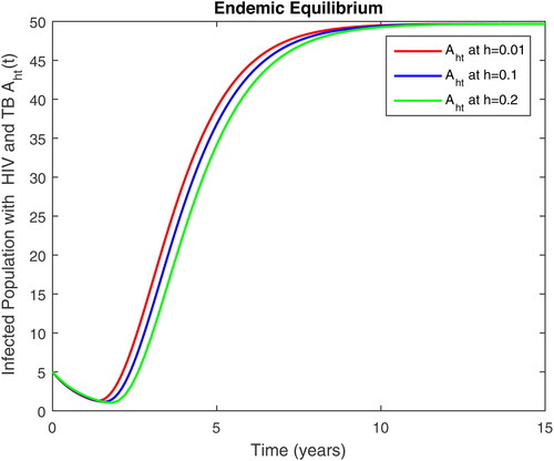
In this section, we present some numerical simulations of susceptible human S, infectious human with TB I_t, infectious human with HIV I_h, infectious human with both of HIV-TB I_ht, infectious human with only HIV and susceptible to TB A_h and infectious human with both HIV and TB A_ht for both case of ${\mathbb{R}}_0^h<1,{\mathbb{R}}_0^t<1$ and ${\mathbb{R}}_0^h>1,{\mathbb{R}}_0^t>1$ using values of associated parameters taken in Tables 1 and 2 respectively. By analyzing the graphical results assure us to justify the theoretical literature review of stability and instability of co-infection of TB-HIV. The following graphical results are plotted by a well-known software MATLAB. By using the NSFD scheme, we draw the graphical solution of the system in Figures 1–6 which will approached to study state points for disease free and in Figures 7–12 for endemic point of the system.

Figure 1. Susceptible population S(t) in time t at different step size for DFE.

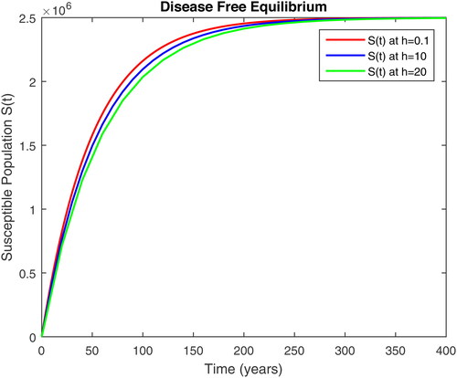
Figure 2. Infected population with TB $I_t(t)$ in time t at different step size for DFE.

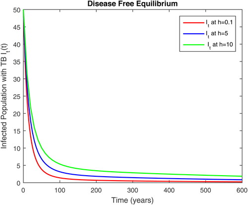
Figure 3. Infected population with HIV only $I_h(t)$ in time t at different step size for DFE.

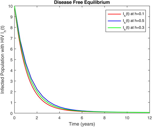
Figure 4. Infected population with both TB and HIV $I_{ht}(t)$ in time t at different step size for DFE.

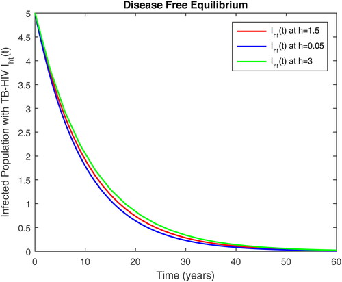
Figure 5. Infected with AIDS only and susceptible to TB class $A_h(t)$ in time t at different step size for DFE.

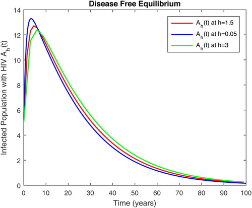
Figure 6. Infected population with TB and AIDS both class $A_{ht}(t)$ in time t at different step size for DFE.

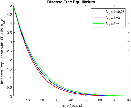
Figure 7. Susceptible population S(t) in time t for EEP at different step size.

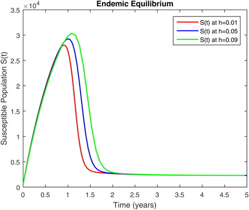
Figure 8. Infected population with TB $I_t(t)$ in time t for EEP at different step size.

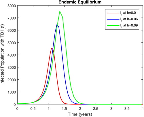
Figure 9. Infected population with HIV only $I_h(t)$ in time t for EEP at different step size.

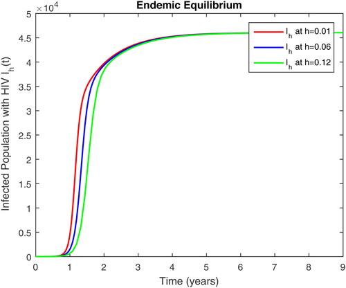
Figure 10. Infected population with both TB and HIV $I_{ht}(t)$ in time t for EEP at different step size.

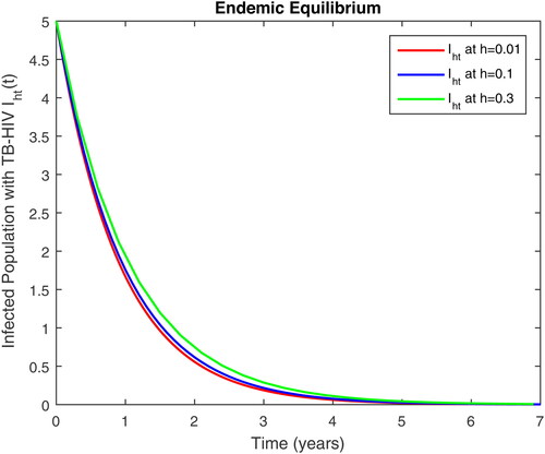
Figure 11. Infected with AIDS only and susceptible to TB class $A_h(t)$ in time t for EEP at different step size.

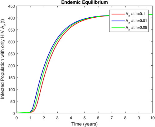
Figure 12. Infected population with TB and AIDS both class $A_{ht}(t)$ in time t for EEP at different step size.

6. Conclusion

In this article, we present a mathematical model for the co-infection of TB and HIV transmission along with variable aggregate population size. The well-posedness of the co-infection TB-HIV model is presented. Furthermore, we analyze the existence of a disease-free and endemic equilibrium for the co-infection of TB-HIV. Also, we present the basic reproduction number ${\mathbb{R}}_0^t$ and ${\mathbb{R}}_0^h$ for Tb and HIV infection respectively. The formulation and sensitivity analysis of fundamental reproduction numbers for Tb and HIV are analyzed. The formulation of the proposed co-infection TB-HIV model in terms of non-standard finite difference schemes is presented. Finally, we present the graphical representation of the solution using the Non-Standard Finite Difference scheme which provides the solution according to our steady-state for both disease-free and endemic equilibrium.

Disclosure statement

No potential conflict of interest was reported by the author(s).

References

- Alexander, M. E., Summers, A. R., & Moghadas, S. M. (2006). Neimark-Sacker bifurcations in a non-standard numerical scheme for a class of positivity preserving ODEs. Proceedings of the Royal Society A: Mathematical, Physical and Engineering Sciences, 462(2074), 3167–3184.
- Alison, L. H. (2018). Mathematical models of HIV latency. Current Topics in Microbiology and Immunology, 417, 131–156.
- Alshabanat, A., Jleli, M., Kumar, S., & Samet, B. (2020). Generalization of Caputo-Fabrizio fractional derivative and applications to electrical circuits. Frontiers in Physics, 8, 64.
- Anderson, R. M., & May, R. M. (1991). Infectious diseases of humans: Dynamics and control. New York: Oxford University Press.
- Arenas, A. J., Parra, G., & Charpentier, C. M. (2010). A nonstandard numerical scheme of predictor-corrector type for epidemic models. Computers & Mathematics with Applications, 59(12), 3740–3749.
- Baleanu, D., Jleli, M., Kumar, S., & Samet, B. (2020). A fractional derivative with two singular kernels and application to a heat conduction problem. Advances in Difference Equations, 2020, 252.
- Farman, M., Ahmad, A., Akgul, A., & Imtiaz, S. (2020). Analysis and dynamical behavior of fractional order cancer model with vaccine strategy. Mathematical Method in the Applied Sciences. doi:10.1002/mma.6240
- Farman, M., Akgul, A., Baleanu, D., Imtiaz, S., & Ahmad, A. (2020). Analysis of fractional order chaotic financial model with minimum interest rate impact. Fractal and Fractional, 4(3), 43.
- Farman, M., Saleem, M. U., Ahmad, A., & Ahmad, M. O. (2018). Analysis and numerical solution of SEIR epidemic model of measles with non-integer time fractional derivatives by using Laplace adomian decomposition method. Ain Shams Engineering Journal, 9(4), 3391–3397.
- Farman, M., Saleem, M. U., Ahmad, A., Imtiaz, S., Tabassum, M. F., Akram, S., & Ahmad, M. O. (2020). A control of glucose level in insulin therapies for the development of artificial pancreas by Atangana Baleanu fractional derivative. Alexandria Engineering Journal, 59(4), 2639–2648.
- Farman, M., Saleem, M. U., Ahmad, M. O., & Ahmad, A. (2018). Stability analysis and control of glucose insulin glucagon system in human. Chines Journal of Physics, 56(4), 1362–1369.
- Farman, M., Saleem, M. U., Tabassum, M. F., Ahmad, A., & Ahmad, M. O. (2019). A linear control of composite model for glucose insulin glucagon. Ain Shamas Engineering Journal, 10(4), 867–872.
- Fatmawati, H. T. (2016). An optimal treatment control of TB HIV coinfection. International Journal of Mathematics and Mathematical Sciences, 2016, 8261208.
- Gonzalez-Parra, G., Arenas, A. J., & Charpentier, B. M. (2010). Combination of nonstandard schemes and Richard son’s extrapolation to improve the numerical solution of population models. Mathematical and Computer Modelling, 52(7–8), 1030–1036.
- Huang, Y., Wu, H., & Acosta, E. P. (2010). Hierarchical Bayesian inference for HIV dynamic differential equation models incorporating multiple treatment factors. Biometrical Journal, 52(4), 470–486. doi:10.1002/bimj.200900173
- Jordan, P. M. (2003). A nonstandard finite difference scheme for nonlinear heat transfer in a thin finite rod. The Journal of Difference Equations and Applications, 9(11), 1015–1021.
- Kumar, S., Ghosh, S., Lotayif, M. S. M., & Samet, B. (2020). A model for describing the velocity of a particle in Brownian motion by Robotnov function based fractional operator. Alexandria Engineering Journal, 59(3), 1435–1449.
- Kumar, S., Ghosh, S., Samet, B., & Goufo, E. F. D. (2020). An analysis for heat equations arises in diffusion process using new Yang Abdel Aty Cattani fractional operator. Mathematical Methods in the Applied Sciences, 43(9), 6062–6080.
- Kumar, S., Kumar, A., Abbas, S., Al Qurashi, M., & Baleanu, D. (2020). A modified analytical approach with existence and uniqueness for fractional Cauchy reaction–diffusion equations. Advances in Difference Equations, 2020(1), 28.
- Kumar, S., Kumar, A., Odibat, Z., Aldhaifallah, M., & Nisar, K. S. (2020). A comparison study of two modified analytical approach for the solution of nonlinear fractional shallow water equations in fluid flow. AIMS Mathematics, 5(4), 3035–3055.
- Kumar, S., Kumar, R., Agarwal, R. P., & Samet, B. (2020). A study of fractional Lotka Volterra population model using Haar wavelet and Adams Bashforth Moulton methods. Mathematical Methods in the Applied Sciences, 43(8), 5564–5578.
- Kumar, S., Kumar, R., Cattani, C., & Samet, B. (2020). Chaotic behaviour of fractional predator-prey dynamical system. Chaos, Solitons and Fractals, 135, 109811.
- Kumar, S., Nisar, K. S., Kumar, R., Cattani, C., & Samet, B. (2020). A new Rabotnov fractional exponential function based fractional derivative for diffusion equation under external force. Mathematical Methods in the Applied Sciences, 43(7), 4460–4471.
- Lawn, S. D., & Zumla, A. I. (2011). Tuberculosis. Lancet, 378(9785), 57–72.
- Mickens, R. (1994). Nonstandard finite difference models of differential equations. Singapore: World Scientific.
- Mickens, R. (2000). Advances in the applications of nonstandard finite difference schemes. Singapore: World Scientific.
- Mickens, R. E. (2005). Advances in the applications of nonstandard finite difference schemes. Singapore: Wiley-Interscience.
- Mickens, R. E. (2007). Calculation of denominator functions for nonstandard finite difference schemes for differential equations satisfying a positivity condition. Numerical Methods for Partial Differential Equations, 23(3), 672–691.
- Nowak, M. A., & May, R. M. C. (2000). Virus dynamics: Mathematical principles of immunology and virology. New York: Oxford University Press.
- Odibat, Z., & Kumar, S. (2019). A robust computational algorithm of homotopy asymptotic method for solving systems of fractional differential equations. Journal of Computational and Nonlinear Dynamics, 14(8), 081004.
- Raza, A., Farman, M., Akgul, A., Iqbal, S., & Ahmad, A. (2020). Simulation and numerical solution of fractional order ebola virus model with novel technique. Bioengineering Journal, 7(4), 194–207.
- Sadegh, Z., & Miehran, N. A. (2015). Nonstandard finite difference scheme for solving fractional-order model of HIV-1 infection of CD4+ T-cells. Iranian Journal of Mathematical Chemistry, 6(2), 169–184.
- Saleem, M. U., Farman, M., Ahmad, A., Ehsan, H., & Ahmad, M. O. (2020). A Caputo Fabrizio fractional order model for control of glucose in insulin therapies for diabetes. Ain Shamas Engineering Journal. doi:10.1016/j.asej.2020.03.006
- Saleem, M. U., Farman, M., Ahmad, M. O., & Rizwan, M. (2017). A control of artificial human pancreas. Chinese Journal of Physics, 55(6), 2273–2282.
- Saleem, M. U., Farman, M., Rizwan, M., Ahmad, M. O., & Ahmad, A. (2018). Controllability and observability of glucose insulin glucagon systems in human. Chinese Journal of Physics, 56(5), 1909–1916.
- Silva, C. J., & Torres, D. F. M. (2018). Global stability for a HIV/AIDS model. Communications Faculty of Sciences University of Ankara Series, 67(1), 93–101.
- Tahir, M., Inayat, A. S., & Zaman, G. (2019). Prevention strategy for superinfection mathematical model tuberculosis and HIV associated with AIDS. Cogent Mathematics and Statistics, 6, 1637166.
- Veeresha, P., Prakasha, D. G., & Kumar, S. (2020). A fractional model for propagation of classical optical solitons by using nonsingular derivative. Mathematical Methods in the Applied Sciences. doi:10.1002/mma.6335