Mathematical modeling for enzyme inhibitors with slow and fast subsystems

Abstract

Mathematical modeling for biochemical enzyme inhibitor systems plays an important role in the systems of biology. Studying and analyzing the dynamical behavior for such models often need some techniques to obtain the model reduction. The well-known techniques of model reduction are suggested in order to divide the model equations into slow and fast subsystems. They are quasi steady-state approximation and quasi-equilibrium approximation. These techniques are great mathematical tools for simplifying model equations and identifying some analytical approximate solutions. In this work, we define mathematical models of enzyme inhibitors and suggest the model reduction approaches. We study two models as examples for enzyme inhibitors such as competitive inhibition and uncompetitive inhibition. Obtained results show that the suggested approaches are effective tools to minimize the number of elements and to find analytical approximate solutions. Accordingly, the idea of separating slow and fast equations will be applied for a wide range of complex enzyme inhibitor networks.

Keywords:

• Mathematical modeling
• enzyme reactions
• slow and fast subsystems
• model reductions

Introduction

Enzyme inhibitors are occurred as molecules. They are involved with catalysis and enzymatic reactions. It is clear that studying of enzyme inhibitors provided a good information about enzyme mechanisms and helped us to define some metabolic pathways. Reversible and irreversible inhibitors are two main important types of enzyme inhibitors. Reversible inhibitors are also classified into three types: competitive inhibitors, uncompetitive inhibitors and mixed inhibitors (Mohan, Long, & Mutneja, 2013).

There are some studies about mathematical tools that have been used to analyze enzymatic reactions such as mathematical modeling for metabolism pathways (Gombert & Nielsen, 2000); simulation and parameter estimation for enzymatic reaction (Özöğür, 2009); kinetic dynamics in heterogeneous enzymatic hydrolysis of cellulose (Gan, Allen, & Taylor, 2003); a mathematical model of dynamics and control in metabolic reaction networks (Palsson, Palsson, & Lightfoot, 1985); a mathematical modeling for metabolic enzyme inhibition (Fang, Wallqvist, & Reifman, 2009), mathematical modeling of metabolism (Giersch, 2000); kinetic equations for reversible enzyme reactions with some analytical approximate solutions (Khoshnaw, 2013).

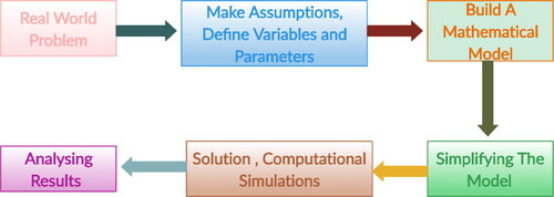
There are a variety of steps that can be used to convert an idea into a theoretical model and then into a quantitative model. It is clear that a theoretical model presents our idea in a model diagram that involving arrows and boxes. Mathematical equations are also used to define the rate of each process (Baker, 2011; Ingalls, 2012; Kot, 2001; Lawson & Glenn, 2008; Murray, 2001; Sontag, 2014). In Figure 1, it can be seen that a series of steps are required to define modeling process.

Figure 1. Mathematical modeling steps.

Mathematical modeling has a great role to describe and analysis models in systems biology. It helps us to understand phenomena in real-world situations. The reader can see many studies in systems biology that mathematical tools have been used. For example, the mathematical analysis of Ebola hemorrhagic fever (Atangana & Goufo, 2014); the model of HIV infection of CD4+ cells (Atangana & Alabaraoye, 2013); the Ebola epidemic model (Area et al., 2015); computational analysis of the model describing HIV infection of CD4 (Atangana, Goufo, & Franc, 2014); the SEIR model with treatment (Almeida, 2018) and modeling the spread of river blindness disease (Atangana & Alqahtani, 2016).

Model reduction is a transformation process on the original system to another system in which the new model contains a smaller number of elements (variables and parameters). We have a variety of techniques of model reduction for systems biology. Methods of model reduction here are very important in systems biology for minimizing chemical reaction parameters and species (Khoshnaw, 2015a; Khoshnaw, Mohammad, & Salih, 2017). In this study, some essential techniques of model reductions are reviewed and applied for some enzymatic reactions.

We consider $n$ reversible reactions which are given below (1) $$\sum _{j=1}^m{a}_{ij} x_j \begin{array}{c}\stackrel{{ k}_{i }^{+}}{\to }\\ \underset{{ k}_i^{-} }{\leftarrow }\end{array} \sum _{j=1}^m{b}_{ij} x_j, i=1,2,\dots ,n$$(1) where $x_j\text{ for }j=1,2,\dots ,m$ are chemical components, $a_{ij}\text{ and }{b}_{ij}$ are stoichiometric coefficients, $k_i^{+}\text{ and }{k}_i^{-}$ are reaction constants. The reaction rates for Equation (1)(1) $$\sum _{j=1}^m{a}_{ij} x_j \begin{array}{c}\stackrel{{ k}_{i }^{+}}{\to }\\ \underset{{ k}_i^{-} }{\leftarrow }\end{array} \sum _{j=1}^m{b}_{ij} x_j, i=1,2,\dots ,n$$(1) based on mass action law are given below: (2) $$v_i=k_i^{+} \prod _{i=1}^n{x}_{j }^{a_{ij}}\left(t\right)-k_i^{-} \prod _{i=1}^n{x}_j^{b_{ij}}\left(t\right), j=1,2,\dots , m$$(2)

Then, the model differential equation can be written (3) $$\frac{dx}{dt}=\sum _{i=1}^n{\pi }_i v_i,$$(3) where $x\in {\mathbb{R}}^m\text{ and }{\pi }_{ij}=b_{ij}-a_{ij}.$

There are some recently published works that give an important step forwards to understand the model reduction techniques and their applications in biochemical reaction networks and system biology. For example, some methods of model reduction for large-scale biological systems are given in the following references (Bartocci & Lió, 2016; Eilertsen & Schnell, 2020; Moayyedi, 2019; Kang, KhudaBukhsh, Koeppl, & Rempała, 2019; Kapteijn, Gascon, & Nijhuis, 2018; Khazaaleh, 2018; Shin & Nguyen, 2017; López Zazueta, Bernard, & Gouzé, 2019; Rahmanzadeh, Asadi, & Atashafrooz, 2020; Snowden, van der Graaf, & Tindall, 2017, 2018).

Simplifying and analyzing the complex enzymatic reactions become a difficult task and some well-known methods have been applied in order to describing their dynamics. Classifying the model equations into slow and fast subsystems plays an important role to describing the model dynamics for such systems. The main problem in this work is identifying the slow and fast reactions for enzyme inhibitor models. Quasi-equilibrium approximation (QEA) and quasi steady-state approximation (QSSA) methods can be used to divide model equations into slow and fast subsystems. We apply the suggested methods on two examples of enzymatic inhibition. When the model equations have higher dimensional elements then applying QEA may not be easy analytically because such models may have many possibilities to identify slow and fast reactions. Interestingly, the main contribution in this study is dividing the model equations into slow and fast subsystems for enzyme inhibitor networks based on some suggested steps. Then, calculating some analytical approximate solutions and slow manifolds play an important step forward in simplifying the complexity for such models.

Slow and fast subsystems

The idea of dividing a set of model equations into slow and fast subsets plays an important role in model reductions. This technique has been used for complex biochemical reaction networks to divide model equations and model reactions into slow and fast subsystems. There are two main approaches that can be applied for such systems (Schnell & Maini, 2002; Segel & Slemrod, 1989). They are called quasi-steady approximation and quasi-equilibrium approximation.

The concept of the quasi–steady state was suggested as a model reduction technique in 1913. Then, there are more explanations about the method that suggested by Briggs and Haldane (1925). It was about the simplest enzyme reaction $E +S \leftrightharpoons ES \to E + P.$ Briggs and Haldane assumed that the total enzyme concentration is very small in compared to the substrate concentration $\left[S\right]$ (Briggs & Haldane, 1925; Khazaaleh, 2018; Khoshnaw, 2015b; Khoshnaw & Rasool, 2019a,b; Li & Li, 2013; Li, Shen, & Li, 2008; Pedersen, Bersani, & Bersani, 2008; Volk, Richardson, Lau, Hall, & Lin, 1977).

Then the method became an important technique of model reductions and model analysis for biochemical reactions. In order to define the method, we simply divide a set of variables $x(t)$ for two sets. The first set is called slow species (basics) $x^s(t).$ The second set is called fast species (fast intermediate) $x^f(t).$ Then, the differential equations of a biochemical reaction model can be divided into two subsystems: (4) $$\frac{d{x}^s}{dt}=g^s \left(x^s\left(t\right), x^f\left(t\right), k\right),$$(4) (5) $$\frac{d{x}^f }{dt}=\frac{1}{ϵ} g^f \left(g^s\left(t\right),g^f\left(t\right),k\right),$$(5) where $x\in {\mathbb{R}}^m, x^s\in {\mathbb{R}}^{m_1}, x^f\in {\mathbb{R}}^{m_2}, k\in {\mathbb{R}}^n\text{ and }m=m_1+m_1.$

The first subsystem (9)(9) $${ h}^i\left(x\right)=b_i,\text{ for }1\le i\le k+p$$(9) is called the slow, while the second one (5)(5) $$\frac{d{x}^f }{dt}=\frac{1}{ϵ} g^f \left(g^s\left(t\right),g^f\left(t\right),k\right),$$(5) is called the fast subsystem. We can analyze fast subsystem (5)(5) $$\frac{d{x}^f }{dt}=\frac{1}{ϵ} g^f \left(g^s\left(t\right),g^f\left(t\right),k\right),$$(5) and the standard singular perturbation method can be also applied (Fenichel, 1979; Jones, 1995; Khoshnaw et al., 2020). We can also calculate a slow manifold of the system from the algebraic equations ${\mathrm{g}}^f(x^s(t),$ $x^f(t))=0$ when $ϵ\to 0.$

The idea of QEA has been proposed as a model reduction method for minimizing the number of variables and parameters. The idea of QEA is that the fast reactions become equilibrium very quickly. In other words, the set of fast reactions will reach equilibrium very quickly compared to set of slow reactions. We consider a system of differential equations of chemical reaction as follows (Khoshnaw, 2015b; Schnell & Maini, 2002; Volk et al., 1977): (6) $$\frac{dx}{dt}=\sum _{s,\mathit{slow}}{\mathcal{R}}^s\left(x,k\right){\gamma }^s+\frac{1}{ϵ}\sum _{f,\mathit{fast}}{\mathcal{R}}^f\left(x,k,t\right){\gamma }^f,$$(6) where $ϵ$ is a small parameter $(0<ϵ\ll 1),$ reaction rates are ${\mathcal{R}}^s$ and ${\mathcal{R}}^f.$ The stoichiometric vectors are ${\gamma }^s$ and ${\gamma }^f.$ Then, the fast subsystem takes the following form (7) $$\frac{dx}{dt}=\frac{1}{ϵ}\sum _{f,\mathit{fast}}{\mathcal{R}}^f\left(x,k,t\right){\gamma }^f.$$(7)

More interestingly, we can calculate the quasi-equilibrium manifold using the following algebraic equations (8) $$\sum _{f,\mathit{fast}}{\mathcal{R}}^f\left(x,k,t\right){\gamma }^f=0,$$(8) (9) $${ h}^i\left(x\right)=b_i,\text{ for }1\le i\le k+p$$(9) where Equation (9)(9) $${ h}^i\left(x\right)=b_i,\text{ for }1\le i\le k+p$$(9) is called linear conservation laws. The reader can also find more details about the suggested techniques and their application for biological and chemical models in Heineken, Tsuchiya, and Aris (1967), Frenzen and Maini (1988), Segel & Martin (1988).

We have also developed some techniques of model reductions recently. They can be used to simplify high dimensional models to smaller sizes in which the dynamics of original models and reduced models should be similar. The suggested approaches geometric singular perturbation method for slow and fast subsystems, and entropy production analysis for identifying non–important reactions. These techniques have been applied to some models in systems biology including enzymatic reactions, elongation factors EF–Tu and EF–Ts signaling pathways, and nuclear receptor signaling (Khoshnaw, 2015a). More recently, an algorithm based on slow and fast reactions was proposed to identify slow and fast reactions in complex systems. It provides a great step further in developing quasi-equilibrium approximation in systems biology. The suggested algorithm was applied to dihydrofolate reductase (DHFR) cell signaling pathways. Results showed that many cell signaling pathways can reach equilibrium in a short interval of time (Khoshnaw & Rasool, 2019a,b). The idea of QSSA may also use to describe the mechanisms of miRNA signaling pathways. This technique is an important tool for separating model equations into slow and fast subsystems. The method provides one to minimize the model elements and to calculate slow manifolds (Khoshnaw & Rasool, 2019a,b).

Competitive inhibition

A competitive inhibitor is the first common type of reversible inhibition, see Figure 2. A competitive inhibitor and substrate are competed for the active site of an enzyme. The active side is occupied by inhibitor (I). It prevents the binding of the substrate to the enzyme (Klonowski, 1983).

Figure 2. Competitive inhibition.

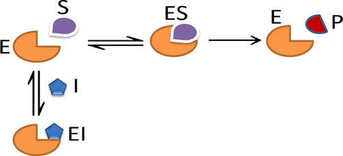
The kinetic reactions of competitive inhibition are given: (10) $$\begin{array}{c} S+E \begin{array}{c}\stackrel{k_1}{\to }\\ \underset{k_2}{\leftarrow }\end{array}\mathit{\text{ ES }}\stackrel{k_3}{\to }E+P,\\ E+I \begin{array}{c}\stackrel{k_4}{\to }\\ \underset{k_5}{\leftarrow }\end{array} EI,\\ \end{array}$$(10) where I is inhibitor, ES and EI are complex intermediate species. The model has five parameters and they are $k_1, k_2, k_3, k_4\text{ and }{k}_5.$ Model variables are $E=\left[E\right], S=\left[S\right], P=\left[P\right], { C}_1=\left[ES\right], C_2=\left[EI\right].$ The model equations can be expressed as follows: (11) $$\begin{array}{c} \frac{dS}{dt}=-k_{1}SE+k_2{C}_1,\\ \frac{dE}{dt}=-k_{1}SE+k_2{C}_1+k_3{C}_1-k_{4}EI+k_5{C}_2,\\ \frac{dI}{dt}=-k_{4}EI+k_5{C}_2,\\ \frac{d{C}_1}{dt}=k_{1}SE-k_2{C}_1-k_3{C}_1,\\ \frac{dp}{dt}=k_3{C}_1,\\ \frac{d{C}_2}{dt}=k_{4}EI-k_5{C}_2.\end{array}$$(11)

We have the following initial conditions (12) $$E\left(0\right)=e_0, S\left(0\right)=s_0, I\left(0\right)=i_0\text{ and }{C}_1\left(0\right)=C_2\left(0\right)=P\left(0\right)=0.$$(12)

The model has the following conservation equations: (13) $$C_2+I=i_0,\mathrm{ }{C}_1+S+P=s_{0 } \mathrm{and} E+C_1+C_2=e_0.$$(13)

By substituting the conservation laws into system (11)(11) $$\begin{array}{c} \frac{dS}{dt}=-k_{1}SE+k_2{C}_1,\\ \frac{dE}{dt}=-k_{1}SE+k_2{C}_1+k_3{C}_1-k_{4}EI+k_5{C}_2,\\ \frac{dI}{dt}=-k_{4}EI+k_5{C}_2,\\ \frac{d{C}_1}{dt}=k_{1}SE-k_2{C}_1-k_3{C}_1,\\ \frac{dp}{dt}=k_3{C}_1,\\ \frac{d{C}_2}{dt}=k_{4}EI-k_5{C}_2.\end{array}$$(11) , the kinetic equations take the form: (14) $$\begin{array}{c}\frac{dS}{dt}=-k_{1}S\left(e_0{-i_0+I-C}_1\right)+k_2{C}_1,\\ \frac{dI}{dt}=-k_{4}I\left(e_0{-i_0+I-C}_1\right)+k_5\left(i_0-I\right),\\ \frac{d{C}_1}{dt}=k_{1}S\left(e_0{-i_0+I-C}_1\right)-\left(k_2+k_3\right)C_1. \end{array}$$(14)

By introducing the following new variables: $$\tau =k_1{e}_{0}t, u\left(\tau \right)=\frac{I\left(t\right)}{i_0}, v\left(\tau \right)=\frac{S\left(t\right)}{s_0},\text{ and }w\left(\tau \right)=\frac{C_1\left(t\right)}{e_0}.$$

Therefore, the system (14)(14) $$\begin{array}{c}\frac{dS}{dt}=-k_{1}S\left(e_0{-i_0+I-C}_1\right)+k_2{C}_1,\\ \frac{dI}{dt}=-k_{4}I\left(e_0{-i_0+I-C}_1\right)+k_5\left(i_0-I\right),\\ \frac{d{C}_1}{dt}=k_{1}S\left(e_0{-i_0+I-C}_1\right)-\left(k_2+k_3\right)C_1. \end{array}$$(14) takes the form: (15) $$\frac{dv}{d\tau }=-v \left(\right(1-w)+{\alpha }_1(u-1\left)\right)+{\alpha }_{2}w,$$(15) (16) $$\frac{du}{d\tau }=-u\left({\alpha }_3\right(1-w)-{\alpha }_4(u-1\left)\right)+{\alpha }_5\left(1-u\right),$$(16) (17) $$ϵ\frac{dw}{d\tau }=v\left(\right(1-w)+{\alpha }_1(u-1\left)\right)-{\alpha }_{6}w,$$(17) $$\text{with initial conditions }u\left(0\right)=1,\text{ and }{v}_1\left(0\right)=v_2\left(0\right)=v_3\left(0\right)=0,$$ where $$ϵ=\frac{e_0}{s_0}, {\alpha }_1=\frac{i_0}{e_0}, {\alpha }_2=\frac{k_2}{s_0{k}_1}, {\alpha }_3=\frac{-k_4}{k_1}, {\alpha }_4=\frac{i_0{k}_4}{e_0{k}_1}, {\alpha }_5=\frac{k_5}{e_0{k}_1}\text{ and }{\alpha }_6=\frac{k_2+k_3}{s_0{k}_1}.$$

It is clear that Equations (15) (16)(16) $$\frac{du}{d\tau }=-u\left({\alpha }_3\right(1-w)-{\alpha }_4(u-1\left)\right)+{\alpha }_5\left(1-u\right),$$(16) and (17)(17) $$ϵ\frac{dw}{d\tau }=v\left(\right(1-w)+{\alpha }_1(u-1\left)\right)-{\alpha }_{6}w,$$(17) can be presented in the slow and fast forms. Therefore, we can use QSSA when $ϵ\to 0,$ then the equations take the form (18) $$\frac{dv}{d\tau }=-v \left(\right(1-w)+{\alpha }_1(u-1\left)\right)+{\alpha }_{2}w,$$(18) (19) $$\frac{du}{d\tau }=-u\left({\alpha }_3\right(1-w)-{\alpha }_4(u-1\left)\right)+{\alpha }_5\left(1-u\right)$$(19) (20) $$0=v\left(\right(1-w)+{\alpha }_1(u-1\left)\right)-{\alpha }_{6}w,$$(20)

Equation (43)(43) $$\frac{dv}{d\tau }=\frac{\left(v+{\alpha }_2\right)v(1-{\alpha }_1(1-u)+{v(\alpha }_1(1-v)-1)(v+{\alpha }_3)}{v+{\alpha }_3}.$$(43) can be solved for $w$ in terms of $u$ and v (21) $$w=\frac{v(1+{\alpha }_1(u-1)}{v+{\alpha }_6}.$$(21)

Thus, the approximate solution for Equations (15)–(17) and the manifold $M_0$ are relatively close. The slow manifold $M_0$ is given (22) $$M_0=\left\{\left(u, v\right): u\text{ and }v\in \left[0,1\right], w=\frac{v(1+{\alpha }_1(u-1)}{v+{\alpha }_6}\right\}.$$(22)

By substituting Equation (21)(21) $$w=\frac{v(1+{\alpha }_1(u-1)}{v+{\alpha }_6}.$$(21) into Equations (18)(18) $$\frac{dv}{d\tau }=-v \left(\right(1-w)+{\alpha }_1(u-1\left)\right)+{\alpha }_{2}w,$$(18) and (19)(19) $$\frac{du}{d\tau }=-u\left({\alpha }_3\right(1-w)-{\alpha }_4(u-1\left)\right)+{\alpha }_5\left(1-u\right)$$(19) , the following differential equation close to the manifold $M_0$ are obtained. (23) $$\frac{dv}{d\tau }=\frac{v\left[\right(v+{\alpha }_2\left)\right(1+{\alpha }_1\left(u-1\right))-(1-{\alpha }_1\left(u-1\right)\left)\right(v+{\alpha }_6\left)\right]}{v+{\alpha }_6}$$(23) (24) $$\frac{du}{d\tau }=\frac{-u{\alpha }_3\left[\right(v+{\alpha }_6)-v1+{\alpha }_1\left(u-1\right))]}{v+{\alpha }_6}+\frac{\left(u-1\right)\left)\right(v+{\alpha }_6\left)\right(u{\alpha }_4-{\alpha }_5)}{v+{\alpha }_6}.$$(24)

Using the technique of QEA for chemical reactions (10)(10) $$\begin{array}{c} S+E \begin{array}{c}\stackrel{k_1}{\to }\\ \underset{k_2}{\leftarrow }\end{array}\mathit{\text{ ES }}\stackrel{k_3}{\to }E+P,\\ E+I \begin{array}{c}\stackrel{k_4}{\to }\\ \underset{k_5}{\leftarrow }\end{array} EI,\\ \end{array}$$(10) , we assume that the first reaction $$E+S \begin{array}{c}\stackrel{k_1}{\to }\\ \underset{k_2}{\leftarrow }\end{array} ES,$$ becomes quasi-equilibrium. It means that the parameters can be given $$k_1=\frac{k^{+}}{ϵ}\text{ and }{k}_2=\frac{k^{-}}{ϵ}\text{ where }{k}^{+}=\frac{k_1{e}_0}{s_0} \text{ and }{k}^{-}=\frac{k_2{e}_0}{s_0}.$$

In other words, $k_1$ and $k_2$ are large constants in comparison with $k_4$ and $k_5.$ Thus, Equation (11)(11) $$\begin{array}{c} \frac{dS}{dt}=-k_{1}SE+k_2{C}_1,\\ \frac{dE}{dt}=-k_{1}SE+k_2{C}_1+k_3{C}_1-k_{4}EI+k_5{C}_2,\\ \frac{dI}{dt}=-k_{4}EI+k_5{C}_2,\\ \frac{d{C}_1}{dt}=k_{1}SE-k_2{C}_1-k_3{C}_1,\\ \frac{dp}{dt}=k_3{C}_1,\\ \frac{d{C}_2}{dt}=k_{4}EI-k_5{C}_2.\end{array}$$(11) takes the form of Equation (6)(6) $$\frac{dx}{dt}=\sum _{s,\mathit{slow}}{\mathcal{R}}^s\left(x,k\right){\gamma }^s+\frac{1}{ϵ}\sum _{f,\mathit{fast}}{\mathcal{R}}^f\left(x,k,t\right){\gamma }^f,$$(6) (25) $$\begin{array}{c}\frac{dS}{dt}=\frac{-1}{ϵ}{g}^f\left(S, E, C_1\right),\\ \frac{dE}{dt}=\frac{-1}{ϵ}{g}^f\left(S, E, C_1\right)+g^{s_1}\left( C_1\right)+g^{s_2}\left(E, I, C_2\right),\\ \frac{dI}{dt}=g^{s_2}\left(E, I, C_2\right),\\ \frac{d{C}_1}{dt}=\frac{1}{ϵ}{g}^f\left(S, E, C_1\right)-g^{s_1}\left(C_1\right),\\ \frac{dP}{dt}=g^{s_1}\left(C_1\right),\\ \frac{d{C}_2}{dt}=-g^{s_2}\left(E, I, C_2\right),\end{array}$$(25) where $g^f(S, E, C_1)$= $k^{+}SE-k^{-}{C}_1,$ $g^{s_1}\left(C_1\right)=k_3{C}_1$ and $g^{s_2}(E, I, C_2)$ = $-k_{4}EI+k_5{C}_2.$

When $ϵ\to 0,$ we can apply the quasi-equilibrium approximation. Therefore, the model has two slow variables. They are given $b_1(S, C_1)=S+C_1$ and $b_2(E,C_1)=E+C_1$. Slow manifold can be expressed from fast reaction rate equation $g^f\left(S, E, C_1\right)=0.$ The model manifold is given below: (26) $$M_0=\left\{\left(S,E,C_1\right)\in R^3:S=\frac{k^{-}{C}_1}{k^{+}E} \right\}.$$(26)

We assume that the slow variables $b_1\text{ and }{b}_2$ are fixed, (27) $$\begin{array}{c}{k}^{+}SE-k^{-}{C}_1=0,\\ S+C_1=b_1,\\ E+C_1=b_2.\end{array}$$(27)

Then, the following quadratic equation for $C_1$ is obtained: (28) $$k^{+}{C_1}^2-\left(k^{+}{b}_1+k^{+}{b}_2+k^{-}\right)C_1+k^{+}{b}_1{b}_2=0.$$(28)

We can solve Equation (28)(28) $$k^{+}{C_1}^2-\left(k^{+}{b}_1+k^{+}{b}_2+k^{-}\right)C_1+k^{+}{b}_1{b}_2=0.$$(28) for $C_1$ and we have $$C_1\left(b_1{, b}_2\right)=\frac{1}{2}[\left(b_1{+ b}_2+\frac{k^{-}}{k^{+}}\right)\pm \sqrt{{\left(b_1{+ b}_2+\frac{k^{-}}{k^{+}}\right)}^2-4b_1{ b}_2 } ].$$

We select a sign “–” in order to have positive concentrations. If $b_1 \to 0 \mathrm{and}$ $b_2 \to 0\text{ then }{C}_1\to 0.$ Moreover, the solution for other variables take the form $$S\left(b_1{, b}_2\right)=b_1-\frac{1}{2}[\left(b_1{+ b}_2+\frac{k^{-}}{k^{+}}\right)-\sqrt{{\left(b_1{+ b}_2+\frac{k^{-}}{k^{+}}\right)}^2-4b_1{ b}_2 } ],$$ $$E\left(b_1{, b}_2\right)=b_2-\frac{1}{2}[\left(b_1{+ b}_2+\frac{k^{-}}{k^{+}}\right)-\sqrt{{\left(b_1{+ b}_2+\frac{k^{-}}{k^{+}}\right)}^2-4b_1{ b}_2} ].$$

Uncompetitive inhibition

Uncompetitive inhibitors are also another common type of reversible inhibition. An uncompetitive inhibitor binds at a site different from the substrate active site and binds only to the ES complex. This type of reaction requires that one or more substrates bind to E before the inhibitor can bind (Mohan et al., 2013); see Figure 3.

Figure 3. Uncompetitive inhibition.

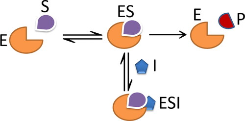
The kinetic reactions of uncompetitive inhibition are given: (29) $$\begin{array}{c}S+E \begin{array}{c}\stackrel{{ k}_{1 }}{\to }\\ \underset{k_2}{\leftarrow }\end{array}\mathit{\text{ ES }}\stackrel{k_3}{\to }E+P,\\ ES+I \begin{array}{c}\stackrel{k_4}{\to }\\ \underset{k_5}{\leftarrow }\end{array} \mathit{ESI},\end{array}$$(29) where I is inhibition; ES and ESI are intermediate components. Model parameters are$k_1, k_2, k_3, k_4\text{and }{k}_5.$ The model variables are $E=\left[E\right], P=\left[P\right], S=\left[S\right], I=\left[I\right], C_1=\left[ES\right], C_2=\left[\mathit{ESI}\right].$ The model differential equations are given based on mass action law (30) $$\begin{array}{c}\frac{dE}{dt}=-k_{1}ES+k_2{c}_1+k_3{C}_1,\\ \frac{dS}{dt}=-k_{1}ES+k_2{C}_1,\\ \frac{d{C}_1}{dt}=k_{1}ES-k_2{C}_1-k_3{C}_1-k_4{C}_{1}I+k_5{C}_2,\\ \frac{dp}{dt}=k_3{C}_1,\\ \frac{dI}{dt}=-k_4{C}_{1}I+k_5{C}_2,\\ \frac{d{C}_2}{dt}=k_4{C}_{1}I-k_5{C}_2,\end{array}$$(30) with the initial conditions (31) $$E\left(0\right)=e_0, S\left(0\right)=s_0\text{ and }I\left(0\right)=i_0, C_1\left(0\right)=C_2\left(0\right)=P\left(0\right)=0.$$(31)

The following three independent stoichiometric conservation laws have obtained from the system (30)(30) $$\begin{array}{c}\frac{dE}{dt}=-k_{1}ES+k_2{c}_1+k_3{C}_1,\\ \frac{dS}{dt}=-k_{1}ES+k_2{C}_1,\\ \frac{d{C}_1}{dt}=k_{1}ES-k_2{C}_1-k_3{C}_1-k_4{C}_{1}I+k_5{C}_2,\\ \frac{dp}{dt}=k_3{C}_1,\\ \frac{dI}{dt}=-k_4{C}_{1}I+k_5{C}_2,\\ \frac{d{C}_2}{dt}=k_4{C}_{1}I-k_5{C}_2,\end{array}$$(30) : (32) $$I+C_2=i_0, C_2+C_1+E=e_0, C_1+P+S+c_2=s_0.$$(32)

By substituting the conservation laws into system (30)(30) $$\begin{array}{c}\frac{dE}{dt}=-k_{1}ES+k_2{c}_1+k_3{C}_1,\\ \frac{dS}{dt}=-k_{1}ES+k_2{C}_1,\\ \frac{d{C}_1}{dt}=k_{1}ES-k_2{C}_1-k_3{C}_1-k_4{C}_{1}I+k_5{C}_2,\\ \frac{dp}{dt}=k_3{C}_1,\\ \frac{dI}{dt}=-k_4{C}_{1}I+k_5{C}_2,\\ \frac{d{C}_2}{dt}=k_4{C}_{1}I-k_5{C}_2,\end{array}$$(30) , the kinetic equations take the form (33) $$\begin{array}{c}\frac{dS}{dt}=-k_{1}S\left(e_0{-i_0+I-C}_1\right)+k_2{C}_1,\\ \frac{d{C}_1}{dt}=k_{1}S\left(e_0{-i_0+I-C}_1\right)-\left(k_2+k_3\right)C_1,\\ \frac{dI}{dt}=-k_4{C}_{1}I+k_5\left(i_0-I\right).\end{array}$$(33)

The following new variables are introduced: $$\tau =k_1{e}_{0}t, u\left(\tau \right)=\frac{I\left(t\right)}{i_0}, v\left(\tau \right)=\frac{S\left(t\right)}{s_0},\text{ and }w\left(\tau \right)=\frac{C_1\left(t\right)}{e_0},$$

Then, system (33)(33) $$\begin{array}{c}\frac{dS}{dt}=-k_{1}S\left(e_0{-i_0+I-C}_1\right)+k_2{C}_1,\\ \frac{d{C}_1}{dt}=k_{1}S\left(e_0{-i_0+I-C}_1\right)-\left(k_2+k_3\right)C_1,\\ \frac{dI}{dt}=-k_4{C}_{1}I+k_5\left(i_0-I\right).\end{array}$$(33) can be expressed as fast and slow subsystems: (34) $$\frac{dv}{d\tau }=-v\left(\right(1-w)-{\alpha }_1(1-v\left)\right)+{\alpha }_{2}w,$$(34) (35) $$ϵ\frac{dw}{d\tau }=v\left(\right(1-w)-{\alpha }_1(1-u\left)\right)-{\alpha }_{3}w,$$(35) (36) $$\frac{du}{d\tau }=-{\alpha }_{4}wu+{\alpha }_5\left(1-u\right),$$(36) where $$ϵ=\frac{e_0}{s_0}, {\alpha }_1=\frac{i_0}{e_0}, {\alpha }_2=\frac{k_2}{s_0{k}_1}, {\alpha }_3=\frac{k_2+k_3}{s_0{k}_1}, {\alpha }_4=\frac{k_4}{k_1}, {\alpha }_5=\frac{k_5}{e_0{k}_1}.$$

With initial conditions $u\left(0\right)=v\left(0\right)=1, w(0)=0.$

When $ϵ\to 0,$ Equations (34)–(36) can be written as follows (37) $$\frac{dv}{d\tau }=-v\left(\right(1-w)-{\alpha }_1(1-v\left)\right)+{\alpha }_{2}w,$$(37) (38) $$0=v\left(\right(1-w)-{\alpha }_1(1-u\left)\right)-{\alpha }_{3}w,$$(38) (39) $$\frac{du}{d\tau }=-{\alpha }_{4}wu+{\alpha }_5\left(1-u\right).$$(39)

We can solve Equation (38)(38) $$0=v\left(\right(1-w)-{\alpha }_1(1-u\left)\right)-{\alpha }_{3}w,$$(38) for $w$ in terms of $v$ and $u$ analytically. It can be given: (40) $$w=\frac{v(1-{\alpha }_1(u-1)}{v+{\alpha }_3}.$$(40)

Furthermore, the approximate solutions and slow manifold are relatively close to each other. The manifold $M_0$ is given below: (41) $$M_0=\left\{\left(u, v, w\right): u\text{ and }v\in \left[0,1\right], w=\frac{v(1-{\alpha }_1(u-1)}{v+{\alpha }_3}\right\}.$$(41)

Therefore, we have nonlinear differential equations and they are close to $M_0$ (42) $$\frac{du}{d\tau }=\frac{-{\alpha }_{4}uv+\left(1-u\right)\left({\alpha }_4{\alpha }_{1}uv+{\alpha }_5(v+{\alpha }_3)\right)}{v+{\alpha }_3},$$(42) (43) $$\frac{dv}{d\tau }=\frac{\left(v+{\alpha }_2\right)v(1-{\alpha }_1(1-u)+{v(\alpha }_1(1-v)-1)(v+{\alpha }_3)}{v+{\alpha }_3}.$$(43)

For QEA of the chemical reactions (29)(29) $$\begin{array}{c}S+E \begin{array}{c}\stackrel{{ k}_{1 }}{\to }\\ \underset{k_2}{\leftarrow }\end{array}\mathit{\text{ ES }}\stackrel{k_3}{\to }E+P,\\ ES+I \begin{array}{c}\stackrel{k_4}{\to }\\ \underset{k_5}{\leftarrow }\end{array} \mathit{ESI},\end{array}$$(29) , we suppose that the second reaction $$ES+I \begin{array}{c}\stackrel{k_4}{\to }\\ \underset{k_5}{\leftarrow }\end{array} \mathit{ESI},$$ goes equilibrium very quickly: $$k_4=\frac{k^{+}}{ϵ}\text{ and }{k}_5=\frac{k^{-}}{ϵ}\text{ where }{k}^{+}=\frac{k_4{e}_0}{s_0}\text{ and }{k}^{-}=\frac{k_5{e}_0}{s_0}.$$

This means $k_4$ and $k_5$ are large constants in compassion with $k_1$ and $k_2.$ Thus, Equation (30)(30) $$\begin{array}{c}\frac{dE}{dt}=-k_{1}ES+k_2{c}_1+k_3{C}_1,\\ \frac{dS}{dt}=-k_{1}ES+k_2{C}_1,\\ \frac{d{C}_1}{dt}=k_{1}ES-k_2{C}_1-k_3{C}_1-k_4{C}_{1}I+k_5{C}_2,\\ \frac{dp}{dt}=k_3{C}_1,\\ \frac{dI}{dt}=-k_4{C}_{1}I+k_5{C}_2,\\ \frac{d{C}_2}{dt}=k_4{C}_{1}I-k_5{C}_2,\end{array}$$(30) has the form of Equation (6)(6) $$\frac{dx}{dt}=\sum _{s,\mathit{slow}}{\mathcal{R}}^s\left(x,k\right){\gamma }^s+\frac{1}{ϵ}\sum _{f,\mathit{fast}}{\mathcal{R}}^f\left(x,k,t\right){\gamma }^f,$$(6) (44) $$\begin{array}{c}\frac{dE}{dt}=g^{s_1}\left(S, E, C_1\right)+g^{s_2}\left(C_1\right),\\ \frac{dS}{dt}=g^{s_1}\left(S, E, C_1\right),\\ \frac{d{C}_1}{dt}=-g^{s_1}\left(S, E, C_1\right)-g^{s_2}\left(C_1\right)+\frac{1}{ϵ}{g}^f\left(C_1,\mathrm{I},C_2\right),\\ \frac{dP}{dt}=g^{s_2}\left(C_1\right),\\ \frac{dI}{dt}=\frac{1}{ϵ}{g}^f\left(C_1,\mathrm{I}, C_2\right),\\ \frac{d{C}_2}{dt}=\frac{-1}{ϵ}{g}^f\left(C_1,\mathrm{I}, C_2\right).\end{array}$$(44) where $g^f(C_1,\mathrm{I},C_2)$ = $-k^{+}{C}_{1}I+k^{-}{C}_2, { g}^{s_1}(S,E,C_1)$= $-k_{1}ES+k_2{C}_1$ and, $g^{s_2}\left( C_1\right)=k_3{C}_1$.

When $ϵ\to 0,$ we can apply the quasi–equilibrium approximation. As a result, the model has two slow variables $b_1(C_1,I)=C_1-I$ and $b_2(I,C_2)=I+C_2.$ The slow manifold is calculated from nonlinear equation $g^f(C_1,\mathrm{I}, C_2)=0.$ This is given by (45) $$M_0=\left\{(C_1,\mathrm{I}, C_2)\in R^2:I=\frac{k^{-}{C}_2}{k^{+}{C}_1}\right\}.$$(45)

After fixing the slow variables $b_1\text{ and }{b}_2,$ we have the following equations (46) $$\begin{array}{c}-k^{+}{C}_{1}I+k^{-}{C}_2=0,\\ C_1-I=b_1,\\ I+C_2=b_2.\end{array}$$(46)

The following quadratic equation for $C_2$ is obtained: (47) $$-k^{+}{C_2}^2+\left(k^{+}{b}_1+2k^{+}{b}_2+k^{-}\right)C_2-k^{+}(b_1+b_2)b_2=0.$$(47)

Equation (47)(47) $$-k^{+}{C_2}^2+\left(k^{+}{b}_1+2k^{+}{b}_2+k^{-}\right)C_2-k^{+}(b_1+b_2)b_2=0.$$(47) can be solved analytically for $C_2.$ We obtain $$C_2\left(b_1{, b}_2\right)=\frac{1}{2}[-\left(b_1{+2 b}_2+\frac{k^{-}}{k^{+}}\right)\pm \sqrt{{\left(b_1{+2 b}_2+\frac{k^{-}}{k^{+}}\right)}^2-4\left(b_1+b_2\right)b_2}].$$

We select a sign “–” in order have positive concentrations of I, $C_1$ and $C_2.$ If $b_1\to 0\text{ and }{b}_2\to 0\text{ then }{C}_2\to 0.$ Moreover, the variables $I\text{ and }{C}_1$ can be also given: $$\begin{array}{c}I\left(b_1{, b}_2\right)=b_2-\frac{1}{2}\left[-\left(b_1{+2 b}_2+\frac{k^{-}}{k^{+}}\right)-\sqrt{{\left(b_1{+2 b}_2+\frac{k^{-}}{k^{+}}\right)}^2-4\left(b_1+b_2\right)b_2}\right],\\ C_1\left(b_1{, b}_2\right)=b_1+b_2-\frac{1}{2}\left[-\left(b_1{+2 b}_2+\frac{k^{-}}{k^{+}}\right)-\sqrt{{\left(b_1{+2 b}_2+\frac{k^{-}}{k^{+}}\right)}^2-4\left(b_1+b_2\right)b_2}\right].\end{array}$$

Conclusions

In this work, we studied some models of enzymatic reactions such as simple enzymatic reactions, competitive inhibition and uncompetitive inhibition. We suggested two methods of model reductions, the first method is quasi-steady-state approximation and the other method is quasi-equilibrium approximation. The suggested model reduction approaches significantly shows an important role in many ways. Firstly, the proposed techniques are very useful tools for reducing the number of elements for such models. Because they allow us to divide the original system into slow and fast subsystems and they can be used to calculate slow manifolds. Another way is that classifying the reaction rates into slow and fast reactions based on quasi-equilibrium approximation is also another important technique in model reduction because it allows us to study species concentrations participated in fast reactions. More interestingly, scaling variables is also used in this study that provides us to calculate some approximate solutions for non-linear enzymatic reaction models. Results in this study will help one to study more about complex enzymatic reactions including enzyme inhibitors. More interestingly, the proposed techniques of model reductions here will be applied to a wide range of complex enzyme inhibitor models in the systems of biology.

References

- Akgül, A., Khoshnaw, S. H., & Rasool, H. M. (2020). Minimizing cell signalling pathway elements using lumping parameters. Alexandria Engineering Journal, 59(4), 2161–2169. doi:10.1016/j.aej.2020.01.041
- Ali, M., Hamza, S., Aldila, D., Sultan, F., Mustafa, S., & Shahzad, M. (n.d.). Evaluation of steady-state to identify the fast-slow completion-route in the multi-route reaction mechanism. 1–6. doi:10.1007/s13204-020-01455-2.
- Almeida, R. (2018). Analysis of a fractional SEIR model with treatment. Applied Mathematics Letters, 84, 56–62. doi:10.1016/j.aml.2018.04.015
- Area, I., Batarfi, H., Losada, J., Nieto, J.J., Shammakh, W., & Torres, Á. (2015). On a fractional order Ebola epidemic model. Advances in Difference Equations, 2015(1). doi:10.1186/s13662-015-0613-5
- Atangana, A., & Alabaraoye, E. (2013). Solving a system of fractional partial differential equations arising in the model of HIV infection of CD4+ cells and attractor one-dimensional Keller–Segel equations. Advances in Difference Equations, 2013(1). doi:10.1186/1687-1847-2013-94
- Atangana, A., & Alqahtani, R.T. (2016). Modelling the spread of river blindness disease via the caputo fractional derivative and the beta-derivative. Entropy, 18(2), 40. doi:10.3390/e18020040
- Atangana, A., & Goufo, E. F. D. (2014). On the mathematical analysis of Ebola hemorrhagic fever: Deathly infection disease in West African countries. BioMed Research International, 2014, 261383–261387. doi:10.1155/2014/261383
- Atangana, A., Goufo, D., & Franc, E. (2014). Computational analysis of the model describing HIV infection of CD4 + T cells. BioMed Research International, 2014, 618404. doi:10.1155/2014/618404
- Baker, R. E. (2011). Mathematical biology and ecology lecture notes. University of Oxford, Oxford.
- Bartocci, E., & Lió, P. (2016). Computational modeling, formal analysis, and tools for systems biology. PLoS Computational Biology, 12(1), e1004591. doi:10.1371/journal.pcbi.1004591
- Briggs, G. E., & Haldane, J. B. (1925). A note on the kinetics of enzyme action. The Biochemical Journal, 19(2), 338–339. doi:10.1042/bj0190338
- Eilertsen, J., & Schnell, S. (2020). The quasi-steady-state approximations revisited: Timescales, small parameters, singularities, and normal forms in enzyme kinetics. Mathematical Biosciences, 325, 108339. doi:10.1016/j.mbs.2020.108339
- Fang, X., Wallqvist, A., & Reifman, J. (2009). A systems biology framework for modeling metabolic enzyme inhibition of Mycobacterium tuberculosis. BMC Systemic Biology, 3(1), 92. doi:10.1186/1752-0509-3-92
- Fenichel, N. (1979). Geometric singular perturbation theory for ordinary differential equations. Journal of Differential Equations, 31(1), 53–98. doi:10.1016/0022-0396(79)90152-9
- Frenzen, C. L., & Maini, P. K. (1988). Enzyme kinetics for a two-step enzymic reaction with comparable initial enzyme–substrate ratios. Journal of Mathematical Biology, 26(6), 689–703. doi:10.1007/BF00276148
- Gan, Q., Allen, S.J., & Taylor, G. (2003). Kinetic dynamics in heterogeneous enzymatic hydrolysis of cellulose: An overview, an experimental study and mathematical modelling. Process Biochemistry, 38(7), 1003–1018. doi:10.1016/S0032-9592(02)00220-0
- Giersch, C. (2000). Mathematical modelling of metabolism. Current Opinion in Plant Biology, 3 (3), 249–253. doi:10.1016/S0958-1669(00)00079-3
- Gombert, A.K., & Nielsen, J. (2000). Mathematical modelling of metabolism. Current Opinion in Biotechnology, 11(2), 180–186. doi:10.1016/S0958-1669(00)00079-3
- Heineken, F. G., Tsuchiya, H. M., & Aris, R. (1967). On the mathematical status of the pseudo-steady state hypothesis of biochemical kinetics. Mathematical Biosciences, 1(1), 95–113. doi:10.1016/0025-5564(67)90029-6
- Ingalls, B. (2012). Mathematical modelling in systems biology: An introduction. University of Waterloo, Waterloo.
- Jones, C. K. (1995). Geometric singular perturbation theory. Dynamical Systems. Lecture Notes in Mathematics, 1609, 44–118. doi:10.1007/BFb0095239
- Kang, H. W., KhudaBukhsh, W. R., Koeppl, H., & Rempała, G. A. (2019). Quasi-steady-state approximations derived from the stochastic model of enzyme kinetics. Bulletin of Mathematical Biology, 81(5), 1303–1336. doi:10.1007/s11538-019-00575-3
- Kapteijn, F., Gascon, J., & Nijhuis, T. A. (2018). Chemical kinetics of catalyzed reactions. Catalysis: An integrated textbook for students. doi:10.1007/978-1-4020-4547-9_6
- Khazaaleh, M. (2018). Two reduction methods to simplify complex ODE mathematical models of biological networks and a case study: The G1/S checkpoint/DNA-damage signal transduction pathways [Doctoral dissertation]. Lincoln University, Lincoln.
- Khoshnaw, S. H. (2013). Iterative approximate solutions of kinetic equations for reversible enzyme reactions. Natural Science, 05(06), 740–755. doi:10.4236/ns.2013.56091
- Khoshnaw, S.H.A. (2015b). Reduction of a kinetic model of active export of importins. Dynamical Systems, Differential Equations & Applications, 705–722. doi:10.3934/proc.2015.0705
- Khoshnaw, S. H. A., Mohammad, N. A., & Salih, R. H. (2017). Identifying critical parameters in SIR model for spread of disease. Open Journal of Modelling & Simulation, 05(01), 32–46. doi:10.4236/ojmsi.2017.51003
- Khoshnaw, S. H. A., & Rasool, H. M. (2019). Model reduction for non-linear protein translation pathways using slow and fast subsystems. Zanco Journal of Pure & Applied Sciences, 31(2), 14–24. doi:10.21271/zjpas.31.2.3
- Khoshnaw, S. H. (2015a). Model reductions in biochemical reaction networks (PhD thesis). University of Leicester, Leicester.
- Khoshnaw, S. H., & Rasool, H. M. (2019). Mathematical Modelling for complex biochemical networks and identification of fast and slow reactions. The international conference on mathematical and related sciences (pp. 55–69). Antalya: Springer. doi:10.1007/s13204-020-01455-2
- Klonowski, W. (1983). Simplifying principles for chemical and enzyme reaction kinetics. Biophysical Chemistry, 18(2), 73–87. doi:10.1016/0301-4622(83)85001-7
- Kot, M. (2001). Elements of mathematical ecology. Cambridge: Cambridge University Press.
- Lawson, D., & Glenn, M. (2008). An introduction to mathematical modeling. Bioinformatics & Statistics Scotland, 3–13.
- Li, B., & Li, B. (2013). Quasi-steady-state laws in reversible model of enzyme kinetics. Journal of Mathematical Chemistry, 51(10), 2668–2686. doi:10.1007/s10910-013-0229-5
- Li, B., Shen, Y., & Li, B. (2008). Quasi-steady-state laws in enzyme kinetics. The Journal of Physical Chemistry: A, 112(11), 2311–2321. doi:10.1021/jp077597q
- López Zazueta, C., Bernard, O., & Gouzé, J. L. (2019). Dynamical reduction of linearized metabolic networks through quasi steady state approximation. AIChE Journal, 65(1), 18–31. doi:10.1002/aic.16406
- Moayyedi, M. K. (2019). Extension ability of reduced order model of unsteady incompressible flows using a combination of POD and Fourier modes. Journal of Applied & Computational Mechanics, 5(1), 1–12. doi:10.22055/JACM.2018.24099.1171
- Mohan, C., Long, K. D., & Mutneja, M. (2013). An introduction to inhibitors and their biological applications, pp. 3–13.
- Murray, J. D. (2001). Mathematical biology: I: An introduction. Berlin: Springer.
- Özöğür, S. (2009). Mathematical modelling of enzymatic reactions, simulation and parameter estimation. Saarbrucken: VDM Verlag.
- Palsson, B.O., Palsson, H., & Lightfoot, E.N. (1985). Mathematical modelling of dynamics and control in metabolic networks. III. Linear reaction sequences. Journal of Theoretical Biology, 113(2), 231–259. doi:10.1016/S0022-5193(85)80226-5
- Pedersen, M. G., Bersani, A. M., & Bersani, E. (2008). Quasi steady-state approximations in complex intracellular signal transduction networks: A word of caution. Journal of Mathematical Chemistry, 43(4), 1318–1344. doi:10.1007/s10910-007-9248-4
- Rahmanzadeh, M., Asadi, T., & Atashafrooz, M. (2020). The development and application of the RCW method for the solution of the Blasius problem. Journal of Applied & Computational Mechanics, 6(1), 105–111. doi:10.22055/JACM.2019.28250.1469
- Schnell, S., & Maini, P. K. (2002). Enzyme kinetics far from the standard quasi-steady-state and equilibrium approximations. Mathematical & Computer Modelling, 35(1–2), 137–144. doi:10.1016/S0895-7177(01)00156-X
- Segel, L. A. (1988). On the validity of the steady state assumption of enzyme kinetics. Bulletin of Mathematical Biology, 50(6), 579–593. doi:10.1016/S0092-8240(88)80057-0
- Segel, I. H., & Martin, R. L. (1988). The general modifier (“allosteric”) unireactant enzyme mechanism: Redundant conditions for reduction of the steady state velocity equation to one that is first degree in substrate and effector. Journal of Theoretical Biology, 135(4), 445–453. doi:10.1016/s0022-5193(88)80269-8
- Segel, L. A., & Slemrod, M. (1989). The quasi-steady-state assumption: A case study in perturbation. SIAM Review, 31(3), 446–477. doi:10.1137/1031091
- Shin, S. Y., & Nguyen, L. K. (2017). Dissecting cell-fate determination through integrated mathematical modeling of the ERK/MAPK signaling pathway. In ERK signaling. Totowa Press: Humana Press.
- Snowden, T. J., van der Graaf, P. H., & Tindall, M. J. (2017). Methods of model reduction for large-scale biological systems: A survey of current methods and trends. Bulletin of Mathematical Biology, 79(7), 1449–1486. doi:10.1007/s11538-017-0277-2
- Snowden, T. J., van der Graaf, P. H., & Tindall, M. J. (2018). Model reduction in mathematical pharmacology: Integration, reduction and linking of PBPK and systems biology models. Journal of Pharmacokinetics & Pharmacodynamics, 45(4), 537–555. doi:10.1007/s10928-018-9584-y
- Sontag, E. D. (2014). Lecture notes on mathematical systems biology. New Brunswick: Rutgers University.
- Volk, L., Richardson, W., Lau, K. H., Hall, M., & Lin, S. H. (1977). Steady state and equilibrium approximations in reaction kinetics. Journal of Chemical Education, 95(2), 95–97. doi:10.1021/ed054p95