Homotopy analysis approach to study the dynamics of fractional deterministic Lotka-Volterra model

Abstract

The population dynamics of two species that is governed by the deterministic Lotka-Volterra model concerned with the interaction of predator and prey is investigated in this article as an application of homotopy analysis method. The analytical approximate solution in the form of convergent infinite series is obtained by considering the time-fractional derivatives in the Caputo sense. The simulation of obtained results exhibit the effect of variation in fractional parameters, auxiliary parameters and auxiliary linear operators on the mass concentration of both the biological species which in turn affects the structure of the system.

Keywords:

• Homotopy analysis method
• Lotka-Volterra model
• Caputo fractional derivative

2010 MATHEMATICS SUBJECT CLASSIFICATION:

• 92D25
• 65L03

1. Introduction and preliminaries

The ecological mathematics has emerged as a subject which has recently attracted the attention of mathematicians and biologists as it helps in understanding the evolution of the ecological system. The Lotka-Volterra model proposed by Lotka (Carmichael & Lotka, 1926) and Volterra (1926) in 1926 is one of the fundamental models in ecology comprising two populations interacting at a time, one being the predator and another being the prey. So, the Lotka-Volterra model is also known as the predator-prey equations. The model describes the struggle for coexistence of two species ensuring the survival of both species for long term and hence paves the way for the abidance of the system.

The predator prey interaction is basically a process that creates disturbances to the system and under simple hypotheses the interaction of two species tends to generate periodic oscillations in reciprocal manner. The predator prey model is a pair of first order coupled ODE’s formulated by simple birth death process.

To specify the model, certain assumptions are made such as:

1. Only two species exist.

2. When predators are absent, prey population grows exponentially. Similarly predator population will starve and lead to exponential death in absence of prey.

3. Prey are primary source of food for predators and can be consumed in infinite quantity by predators.

4. In a homogeneous environment both populations can move randomly with-out any complexity. With these assumptions, the predator-prey populations are governed by the pair of equations: $$\begin{array}{c}\frac{dx}{dt}=\alpha x-\beta xy,\\ \frac{dy}{dt}=\delta xy-\gamma y,\end{array}$$ where x and y are the cardinality of prey and predator respectively. $\alpha , \beta , \gamma , \delta$ are positive real parameters signifying the interaction between the two species.

Recently, many researchers have studied the traditional Lotka-Volterra models with various modifications. A simple high-dimensional Lotka-Volterra model exhibiting spatiotemporal chaos in one spatial dimension is described by Sprott, Wildenberg, and Azizi (2005), Xiao and Ruan (2001b). Tiwana, Maqbool, and Mann (2017) studied the global dynamics of a ratio-dependent system. In which they use homotopy perturbation Laplace transform method to solve the fractional non-linear reaction diffusion system of Lotka-Volterra type differential equation. This can be considered as predator-prey System. Qualitative behaviour of a predator-prey system with nonmonotonic functional response with a series of bifurcations is discussed by Xiao and Ruan (2001a). Maiti, Sen, and Samanta (2016) analyzed the deterministic and stochastic prey–predator model with herd behaviour in both. Integro-differential equations for Lotka-Volterra model were derived by Anisiu (2014). The Holling type-II Lotka-Volterra predator-prey system with impulsive immigration of predator has been studied by Liu and Chen (2003). Fractional Lotka-Volterra population model using Haar wavelet and Adams-Bashforth-Moulton methods was given by Kumar, Kumar, Agarwal, & Samet (2020). Stability analysis for deterministic and stochastic fluctuations of a predator-prey model has been done by Addison (2017).

Recently, numerous models in biology (Dave, Khan, Purohit, & Suthar, 2021; Khan, Purohit, Dave, & Suthar, 2021; Mistry, Khan, & Suthar, 2020), and dynamics (Alaria, Khan, Suthar, & Kumar, 2019) can be modelled with the help of fractional order derivatives. In the past few years, many researchers have been established and applied numerous schemes to gain the solutions of fractional order differential equations such as Abeye, Ayalew, Suthar, Purohit, and Jangid (2022), Ramani, Khan, and Suthar (2019), and Ramani, Khan, Suthar, and Kumar (2022). Homotopy analysis method has been applied successfully by the researchers to find approximate solutions of fractional nonlinear partial differential equations (Agarwal, Yadav, Albalawi, Nisar, & Shefeeq, 2022; Hassani, Tabar, Nemati, Domairry, & Noori, 2011; Nassar, Revelli, & Bowman, 2011; Pareek, Gupta, Agarwal, & Suthar, 2021; Song & Zhang, 2007; Wu, Wang, & Liao, 2005; Zurigat, Momani, Odibat, & Alawneh, 2010; Yadav, Agarwal, Suthar & Purohit, 2022) as it is not easy to attain the exact solution of these equations. Also HAM has an advantage over other techniques to control the convergence region of the solution by choosing the auxiliary parameter arbitrarily.

This paper is organized as follows. In Sec. 2, we discussed some fractional calculus theory which has been used in the main findings. In Sec. 3, HAM is implemented to solve the fractional deterministic model of Lotka-Volterra type and analytic approximate solution is also found in the form of infinite series. In Sec. 4, the numerical analysis for fractional and auxiliary parameters has also been done. Finally, in Sec. 5 is concerned with the conclusion.

2. Basic definitions

In this part, we will review some fundamental properties of fractional calculus theory that will be useful in our work (Agarwal, Kritika, & Purohit, 2021; Agarwal, Kritika, Purohit, & Kumar, 2021; Dave et al., 2021; Ghanbari, Kumar, & Kumar, 2020; Kritika & Agarwal, 2020; Kumar, Kumar, Samet, Gómez-Aguilar, and Osman, 2020; Miller & Ross, 1993; Oldham & Spanier, 1974; Podlubny, 1999; Suthar, Purohit, & Araci, 2020; Veeresha, Prakasha, & Kumar, 2020):

Definition 2.1.

If $\aleph (x),x>0$ is a real valued function, then it is said to be in the space $C_{\mu },\mu \in \mathfrak{R}$ if $\exists$ $p>\mu$ s.t.: $$\aleph (x)=x^p{\aleph }_{1}x$$ where ${\aleph }_1(x)\in C[0,\infty \}.$

Definition 2.2.

If $\aleph (x),x>0$ is a real valued function, then it is said to be in the space $C_{\mu }^n,m\in N\cup \left\{0\right\},if{\aleph }^{(m)}\in C_{\mu }.$

Definition 2.3.

The Riemann-Liouville fractional integral operator of order $\propto \ge 0,$ for a function $\aleph \in C_{\mu },\mu \ge 1$ is $$\begin{array}{c}{J}^{\propto }\aleph \left(x\right)=\frac{1}{\Gamma (\propto )}{\int }_0^x\begin{array}{c}{\left(x-t\right)}^{\propto -1}\aleph \left(t\right)dt;(\propto >0,x>0),\end{array}\\ J^0\aleph \left(x\right)=\aleph (x).\end{array}$$

Which follows the properties: $$\begin{array}{c}{J}^{\propto }{J}^{\beta }\aleph \left(x\right)=J^{\propto +\beta }\aleph \left(x\right),\\ J^{\propto }{x}^{\beta }=\frac{\Gamma (\beta +1)}{\Gamma (\propto +\beta +1)}{x}^{\alpha +\beta }.\end{array}$$

Definition 2.4.

The Caputo’s sense fractional derivative of $\aleph \in C_{-1}^n$ is: $$D^{\propto }\aleph \left(t\right)=\{\begin{array}{c}\frac{1}{\Gamma \left(n-\propto \right)}{\int }_0^t{\left(t-\tau \right)}^{n-\alpha -1}{\aleph }^n\left(\tau \right)d\tau ,n-1<\alpha <n,n\in N^{*},\\ \frac{d^n}{d{t}^n}\aleph \left(t\right),\propto =n.\end{array}$$ and $$D^{\propto }K=0;K\mathrm{is}\mathrm{a}\mathrm{constant},$$ $$D^{\propto }{t}^{\beta }=\{\begin{array}{c}\frac{\Gamma \left(\beta +1\right)}{\Gamma \left(\beta -\propto +1\right)}{t}^{\beta -\alpha } \beta >\alpha -1,\\ 0,\beta \le \alpha -1.\end{array}$$

3. Homotopy analysis methodology for fractional nonlinear PDE’s

HAM for nonlinear systems can be explained by the following equation: (3.1) $$N_i[u_i(t)]=0,$$(3.1) where N_i and u_i are nonlinear operators and unknown functions respectively and t is the independent variables. By ignoring all boundary or initial condition, the zeroth-order deformation equation can be constructed as: (3.2) $$(1-p)L_i[{\varphi }_i(t,p)-u_{i0}(t)]=p{h}_i{H}_i(t)N_i[{\varphi }_i(t,p)],$$(3.2) where $p\in [0,1]$ is an embedding parameter, h_i $\ne$ 0 are auxiliary parameters, L_i are auxiliary linear operators, ${\varphi }_i(t,p)$ are unknown function, $u_{i0}$ (t) are an initial guesses of u_i (t) and H_i (t) $\ne 0$ denote nonzero auxiliary functions.

At p = 0 and p = 1, Eq. (3.2)(3.2) $$(1-p)L_i[{\varphi }_i(t,p)-u_{i0}(t)]=p{h}_i{H}_i(t)N_i[{\varphi }_i(t,p)],$$(3.2) reduced into (3.3) $${\varphi }_i(t,0)=u_{i0}(t),{\varphi }_i(t,1)=u_i(t).$$(3.3)

Thus as p increases from 0 to 1, the solution varies from the initial guess $u_{i0}(t)$ to the solution $u_i(t).$ Expanding ${\varphi }_i(t,p)$ in Taylor series with respect to p, $${\varphi }_i\left(t,p\right)=u_{i0}\left(t\right)+\sum _{m=1}^{\infty }{u}_{im}\left(t\right)p^m,$$ where (3.4) $$u_{im}\left(t\right)=\frac{1}{m!}\frac{{\partial }^m{\varphi }_i\left(t,p\right)}{\partial q^m}$$(3.4)

The convergence of the series in (3.4)(3.4) $$u_{im}\left(t\right)=\frac{1}{m!}\frac{{\partial }^m{\varphi }_i\left(t,p\right)}{\partial q^m}$$(3.4) depends upon the auxiliary parameters $h_i$ and the auxiliary function $s{H}_i(t).$ If it is convergent at $p=1,$ we have (3.5) $$u_i\left(t\right)=u_{i0}\left(t\right)+\sum _{m=1}^{\infty }{u}_{im}\left(t\right).$$(3.5) which is definitely one of the solutions of the nonlinear system considered in (3.1)(3.1) $$N_i[u_i(t)]=0,$$(3.1) , as proven by Liao (1997, 2004) and Goufo et al. (Doungmo Goufo, Kumar, & Mugisha, 2020).

Defining the vector $$\overrightarrow{u_i}=(u_{i0}\left(t\right),u_{i1}\left(t\right),\dots ,u_{in}\left(t\right)).$$

The mth order deformation equation can be written as (3.6) $$L_i[u_{im}\left(t\right)-{\chi }_m{u}_{i(m-1)}(t)]=h_i{H}_i\left(t\right)R_{im}\left[\overrightarrow{u_{i(m-1)}}(t)\right]$$(3.6)

Subject to the initial condition $$u_{im}\left(0\right)=0,$$ where $$\begin{array}{c}{R}_{im}\left[\overrightarrow{u_{i(m-1)}}(t)\right]=\frac{1}{(\mathrm{m}-1)!}\frac{{\partial }^{\mathrm{m}-1}{N}_i\left[{\varphi }_i\left(\mathrm{t},\mathrm{p}\right)\right]}{\partial {\mathrm{p}}^{\mathrm{m}-1}}\\ {\chi }_m=\{\begin{array}{cc}0,& m\le 1\\ 1,& m>1.\end{array}\end{array}$$

If we choose $L_i=D^{{\alpha }_i},$ then according to (3.6)(3.6) $$L_i[u_{im}\left(t\right)-{\chi }_m{u}_{i(m-1)}(t)]=h_i{H}_i\left(t\right)R_{im}\left[\overrightarrow{u_{i(m-1)}}(t)\right]$$(3.6) , we have $$J^{{\alpha }_i}{D}^{{\alpha }_i}\left[u_{im}\left(t\right)-{\chi }_m{u}_{i(m-1)}(t)\right]=h_i{J}^{{\alpha }_i}\left[H_i\left(t\right)R_{im}\left\{\overrightarrow{u_{i(m-1)}}\left(t\right)\right\}\right],$$ which further gives (3.7) $$u_{im}\left(t\right)={\chi }_m{u}_{i(m-1)}\left(t\right)+h_i{J}^{{\alpha }_i}\left[H_i\left(t\right)R_{im}\left\{\overrightarrow{u_{i(m-1)}}\left(t\right)\right\}\right],$$(3.7) subject to the initial condition: $$u_{im}\left(0\right)=0.$$

For the special case when α = 1, (3.6)(3.6) $$L_i[u_{im}\left(t\right)-{\chi }_m{u}_{i(m-1)}(t)]=h_i{H}_i\left(t\right)R_{im}\left[\overrightarrow{u_{i(m-1)}}(t)\right]$$(3.6) reduces to (3.8) $$u_{im}\left(t\right)={\chi }_m{u}_{i(m-1)}\left(t\right)+h_i{\int }_0^t\left[H_i\left(t\right)R_{im}\left\{\overrightarrow{u_{i(m-1)}}\left(t\right)\right\}\right]d\tau .$$(3.8)

4. Numerical solution of Lotka-Volterra model

Consider the Lotka-Volterra model of predator-prey coupled time fraction differential equations given by (4.1) $$\begin{array}{c}{D}_t^{p}x=\alpha x-\beta xy,\\ D_t^{q}y=\delta xy-\gamma y,\end{array}$$(4.1) where $0<p,q\le 1,$ p and $q$ are the time fractional parameters for prey and predator equations respectively, where x and y are the cardinality of prey and predator respectively. $\alpha , \beta , \gamma , \delta$ are positive real parameters denoting the natural growth rate of prey in the absence of predation, predation impact coefficient for prey, natural death rate of predators in absence of prey and coefficient of efficiency of predation respectively.

In order to solve (4.1)(4.1) $$\begin{array}{c}{D}_t^{p}x=\alpha x-\beta xy,\\ D_t^{q}y=\delta xy-\gamma y,\end{array}$$(4.1) using HAM, let the auxiliary linear operators $L_i=\frac{d}{dt},$ auxiliary functions $H_1(t)=H_2(t)=1$ and the initial guesses for the prey and predator population be $x_0(t)=80$ and $y_0(t)=30.$

Now, the homotopy for the system of Eq. (4.1)(4.1) $$\begin{array}{c}{D}_t^{p}x=\alpha x-\beta xy,\\ D_t^{q}y=\delta xy-\gamma y,\end{array}$$(4.1) can be constructed as (4.2) $$\begin{array}{c}{R}_{1m}\left[\overrightarrow{x_{m-1}}(t)\right]=D^p{x}_{m-1}\left(t\right)-\alpha x_{m-1}\left(t\right)+\beta \sum _{i=0}^{m-1}{x}_i\left(t\right)y_{m-i-1}(t),\\ R_{2m}\left[\overrightarrow{y_{m-1}}(t)\right]=D^p{y}_{m-1}\left(t\right)-\delta \sum _{i=0}^{m-1}{x}_i\left(t\right)y_{m-i-1}(t)+\gamma y_{m-1}\left(t\right),\end{array}$$(4.2) and accordingly by HAM, we have (4.3) $$\begin{array}{c}{x}_m(\mathrm{t})={\chi }_m{x}_{m-1}\left(t\right)+h_1{\int }_0^t{R}_{1m}\left[\overrightarrow{x_{m-1}}(\tau )\right]d\tau ,\\ y_m(\mathrm{t})={\chi }_m{y}_{m-1}\left(t\right)+h_2{\int }_0^t{R}_{2m}\left[\overrightarrow{y_{m-1}}(\tau )\right]d\tau .\end{array}$$(4.3)

Solving by HAM, the first few terms of the series solution for (4.1)(4.1) $$\begin{array}{c}{D}_t^{p}x=\alpha x-\beta xy,\\ D_t^{q}y=\delta xy-\gamma y,\end{array}$$(4.1) are as follows: (4.4) $$\begin{array}{c}{x}_0=80,y_0=30,\\ x_1=-80h_1\left(\alpha -30\beta \right)t,y_1=30h_2(\gamma -80\delta )t,\\ x_2=-80h_1\left(\alpha -30\beta \right)t+40h_1{}^2{\left(\alpha -30\beta \right)}^2{t}^2\\ +1200\beta h_1{h}_2\left(\gamma -80\delta \right)t^2-80h_1{}^2\left(\alpha -30\beta \right)\frac{t^{2-p}}{\Gamma (3-p)},\\ y_2=30h_2\left(\gamma -80\delta \right)t+15h_2{}^2{\left(\gamma -80\delta \right)}^2{t}^2\\ +1200\delta h_1{h}_2\left(\alpha -30\beta \right)t^2+30h_2{}^2\left(\gamma -80\delta \right)\frac{t^{2-q}}{\Gamma (3-q)},\\ x_3=-80h_1\left(\alpha -30\beta \right)t+\left\{80h_1{}^2{\left(\alpha -30\beta \right)}^2+2400\beta h_1{h}_2\left(\gamma -80\delta \right)\right\}{t}^2\\ +\{-40h_1{}^3{\left(\alpha -30\beta \right)}^3-3600\beta h_1{}^2{h}_2\left(\gamma -80\delta \right)\left(\alpha -30\beta \right)\\ +1200\beta h_1{h}_2{}^2{\left(\gamma -80\delta \right)}^2+96000\beta \delta h_1{}^2{h}_2\left(\alpha -30\beta \right)\}\frac{t^3}{3}\\ +\left\{-160h_1{}^2\left(\alpha -30\beta \right)\right\}\frac{t^{2-p}}{\Gamma (3-p)}\\ +\left\{160h_1{}^3{\left(\alpha -30\beta \right)}^2+2400\beta h_1{}^2{h}_2\left(\gamma -80\delta \right)\right\}\frac{t^{3-p}}{\Gamma (4-p)}\\ +\left\{-80h_1{}^3\left(\alpha -30\beta \right)\right\}\frac{t^{3-2p}}{\Gamma (4-2p)}+\left\{2400\beta h_1{h}_2{}^2\left(\gamma -80\delta \right)\right\}\frac{t^{3-q}}{\Gamma (4-q)},\\ y_3=30h_2\left(\gamma -80\delta \right)t+\left\{30h_2{}^2{\left(\gamma -80\delta \right)}^2+2400\delta h_1{h}_2\left(\alpha -30\beta \right)\right\}{t}^2\\ +\{15h_2{}^3{\left(\gamma -80\delta \right)}^3+3600h_1{h}_2{}^2\delta \left(\gamma -80\delta \right)\left(\alpha -30\beta \right)-1200\delta h_1{}^2{h}_2{\left(\alpha -30\beta \right)}^2\\ -36000\beta \delta h_1{h}_2{}^2\left(\gamma -80\delta \right)\}\frac{t^3}{3}+\left\{60h_2{}^2\left(\gamma -80\delta \right)\right\}\frac{t^{2-q}}{\Gamma (3-q)}\\ +\left\{60h_2{}^3{\left(\gamma -80\delta \right)}^2+2400\delta h_1{}^2{h}_2\left(\alpha -30\beta \right)\right\}\frac{t^{3-p}}{\Gamma (4-p)}\\ +\left\{30h_2{}^3\left(\gamma -80\delta \right)\right\}\frac{t^{3-2q}}{\Gamma (4-2q)}+\left\{2400\delta h_1{}^2{h}_2\left(\alpha -30\beta \right)\right\}\frac{t^{3-p}}{\Gamma (4-p)}\end{array}$$(4.4) and so on.

Now taking the auxiliary linear operators $L_1=D^p$ and $L_2=D^q$ for the system (4.1)(4.1) $$\begin{array}{c}{D}_t^{p}x=\alpha x-\beta xy,\\ D_t^{q}y=\delta xy-\gamma y,\end{array}$$(4.1) , then the homotopy is written as $$\begin{array}{c}{x}_m(\mathrm{t})={\chi }_m{x}_{m-1}\left(t\right)+h_1{J}^p\left[R_{1m}\left(\overrightarrow{x_{m-1}}(\tau )\right)\right],\\ y_m(\mathrm{t})={\chi }_m{y}_{m-1}\left(t\right)+h_2{J}^q\left[R_{2m}\left(\overrightarrow{y_{m-1}}(\tau )\right)\right].\end{array}$$

For this case, we get the consecutive terms of the series solution as (4.5) $$\begin{array}{c}{x}_0=80,y_0=30,\\ x_1=-80h_1\left(\alpha -30\beta \right)\frac{t^p}{\Gamma (1+p)},y_1=30h_2(\gamma -80\delta )\frac{t^q}{\Gamma (1+q)},\\ x_2=-80h_1\left(1+h_1\right)\left(\alpha -30\beta \right)\frac{t^p}{\Gamma (1+p)}+80h_1{}^2{\left(\alpha -30\beta \right)}^2\frac{t^{2p}}{\Gamma (1+2p)}\\ +2400\beta h_1{h}_2\left(\gamma -80\delta \right)\frac{t^{p+q}}{\Gamma (1+p+q)},\\ y_2=30h_2\left(1+h_2\right)\left(\gamma -80\delta \right)\frac{t^q}{\Gamma (1+q)}+30h_2{}^2{\left(\gamma -80\delta \right)}^2\frac{t^{2q}}{\Gamma (1+2q)}\\ +2400\delta h_1{h}_2\left(\alpha -30\beta \right)\frac{t^{p+q}}{\Gamma (1+p+q)},\\ x_3=-80h_1{\left(1+h_1\right)}^2\left(\alpha -30\beta \right)\frac{t^p}{\Gamma (1+p)}+\left\{160h_1{}^2\left(1+h_1\right){\left(\alpha -30\beta \right)}^2\right\}\frac{t^{2p}}{\Gamma (1+2p)}\\ +\left\{-80h_1{}^3{\left(\alpha -30\beta \right)}^3\right\}\frac{t^{3p}}{\Gamma (1+3p)}+\left\{2400\beta h_1{h}_2\left(2+h_1+h_2\right)\left(\gamma -80\delta \right)\right\}\frac{t^{p+q}}{\Gamma (1+p+q)}\\ +\left\{2400\beta h_1{h}_2{}^2{\left(\gamma -80\delta \right)}^2\right\}\frac{t^{p+2q}}{\Gamma (1+p+2q)}+\left\{-2400\beta h_1{}^2{h}_2\left(\gamma -80\delta \right)\left(\alpha -30\beta \right)\right\}\\ \left\{1+\frac{\Gamma (1+p+q)}{\Gamma (1+p)\Gamma (1+q)}-\frac{80\delta }{\left(\gamma -80\delta \right)}\right\}\frac{t^{2p+q}}{\Gamma (1+2p+q)},\\ y_3=30h_2{\left(1+h_2\right)}^2\left(\gamma -80\delta \right)\frac{t^q}{\Gamma (1+q)}+\left\{60h_2{}^2\left(1+h_2\right){\left(\gamma -80\delta \right)}^2\right\}\frac{t^{2q}}{\Gamma (1+2q)}\\ +\left\{30h_2{}^3{\left(\gamma -80\delta \right)}^3\right\}\frac{t^{3q}}{\Gamma (1+3q)}+\left\{2400\delta h_1{h}_2\left(2+h_1+h_2\right)\left(\alpha -30\beta \right)\right\}\frac{t^{p+q}}{\Gamma (1+p+q)}\\ +\left\{-2400\delta h_1{}^2{h}_2{\left(\alpha -30\beta \right)}^2\right\}\frac{t^{2p+q}}{\Gamma (1+2p+q)}+\left\{2400\delta h_1{h}_2{}^2\left(\gamma -80\delta \right)\left(\alpha -30\beta \right)\right\}\\ \left\{1+\frac{\Gamma (1+p+q)}{\Gamma (1+p)\Gamma (1+q)}-\frac{30\beta }{\left(\alpha -30\beta \right)}\right\}\frac{t^{p+2q}}{\Gamma (1+p+2q)}\end{array}$$(4.5)

and so on.

Here we have taken only first four terms of the infinite series to construct the numerical solution of (4.1)(4.1) $$\begin{array}{c}{D}_t^{p}x=\alpha x-\beta xy,\\ D_t^{q}y=\delta xy-\gamma y,\end{array}$$(4.1) , but further terms can also be found to improve the solution.

The graphical results for the solutions obtained in (4.4)(4.4) $$\begin{array}{c}{x}_0=80,y_0=30,\\ x_1=-80h_1\left(\alpha -30\beta \right)t,y_1=30h_2(\gamma -80\delta )t,\\ x_2=-80h_1\left(\alpha -30\beta \right)t+40h_1{}^2{\left(\alpha -30\beta \right)}^2{t}^2\\ +1200\beta h_1{h}_2\left(\gamma -80\delta \right)t^2-80h_1{}^2\left(\alpha -30\beta \right)\frac{t^{2-p}}{\Gamma (3-p)},\\ y_2=30h_2\left(\gamma -80\delta \right)t+15h_2{}^2{\left(\gamma -80\delta \right)}^2{t}^2\\ +1200\delta h_1{h}_2\left(\alpha -30\beta \right)t^2+30h_2{}^2\left(\gamma -80\delta \right)\frac{t^{2-q}}{\Gamma (3-q)},\\ x_3=-80h_1\left(\alpha -30\beta \right)t+\left\{80h_1{}^2{\left(\alpha -30\beta \right)}^2+2400\beta h_1{h}_2\left(\gamma -80\delta \right)\right\}{t}^2\\ +\{-40h_1{}^3{\left(\alpha -30\beta \right)}^3-3600\beta h_1{}^2{h}_2\left(\gamma -80\delta \right)\left(\alpha -30\beta \right)\\ +1200\beta h_1{h}_2{}^2{\left(\gamma -80\delta \right)}^2+96000\beta \delta h_1{}^2{h}_2\left(\alpha -30\beta \right)\}\frac{t^3}{3}\\ +\left\{-160h_1{}^2\left(\alpha -30\beta \right)\right\}\frac{t^{2-p}}{\Gamma (3-p)}\\ +\left\{160h_1{}^3{\left(\alpha -30\beta \right)}^2+2400\beta h_1{}^2{h}_2\left(\gamma -80\delta \right)\right\}\frac{t^{3-p}}{\Gamma (4-p)}\\ +\left\{-80h_1{}^3\left(\alpha -30\beta \right)\right\}\frac{t^{3-2p}}{\Gamma (4-2p)}+\left\{2400\beta h_1{h}_2{}^2\left(\gamma -80\delta \right)\right\}\frac{t^{3-q}}{\Gamma (4-q)},\\ y_3=30h_2\left(\gamma -80\delta \right)t+\left\{30h_2{}^2{\left(\gamma -80\delta \right)}^2+2400\delta h_1{h}_2\left(\alpha -30\beta \right)\right\}{t}^2\\ +\{15h_2{}^3{\left(\gamma -80\delta \right)}^3+3600h_1{h}_2{}^2\delta \left(\gamma -80\delta \right)\left(\alpha -30\beta \right)-1200\delta h_1{}^2{h}_2{\left(\alpha -30\beta \right)}^2\\ -36000\beta \delta h_1{h}_2{}^2\left(\gamma -80\delta \right)\}\frac{t^3}{3}+\left\{60h_2{}^2\left(\gamma -80\delta \right)\right\}\frac{t^{2-q}}{\Gamma (3-q)}\\ +\left\{60h_2{}^3{\left(\gamma -80\delta \right)}^2+2400\delta h_1{}^2{h}_2\left(\alpha -30\beta \right)\right\}\frac{t^{3-p}}{\Gamma (4-p)}\\ +\left\{30h_2{}^3\left(\gamma -80\delta \right)\right\}\frac{t^{3-2q}}{\Gamma (4-2q)}+\left\{2400\delta h_1{}^2{h}_2\left(\alpha -30\beta \right)\right\}\frac{t^{3-p}}{\Gamma (4-p)}\end{array}$$(4.4) and (4.5)(4.5) $$\begin{array}{c}{x}_0=80,y_0=30,\\ x_1=-80h_1\left(\alpha -30\beta \right)\frac{t^p}{\Gamma (1+p)},y_1=30h_2(\gamma -80\delta )\frac{t^q}{\Gamma (1+q)},\\ x_2=-80h_1\left(1+h_1\right)\left(\alpha -30\beta \right)\frac{t^p}{\Gamma (1+p)}+80h_1{}^2{\left(\alpha -30\beta \right)}^2\frac{t^{2p}}{\Gamma (1+2p)}\\ +2400\beta h_1{h}_2\left(\gamma -80\delta \right)\frac{t^{p+q}}{\Gamma (1+p+q)},\\ y_2=30h_2\left(1+h_2\right)\left(\gamma -80\delta \right)\frac{t^q}{\Gamma (1+q)}+30h_2{}^2{\left(\gamma -80\delta \right)}^2\frac{t^{2q}}{\Gamma (1+2q)}\\ +2400\delta h_1{h}_2\left(\alpha -30\beta \right)\frac{t^{p+q}}{\Gamma (1+p+q)},\\ x_3=-80h_1{\left(1+h_1\right)}^2\left(\alpha -30\beta \right)\frac{t^p}{\Gamma (1+p)}+\left\{160h_1{}^2\left(1+h_1\right){\left(\alpha -30\beta \right)}^2\right\}\frac{t^{2p}}{\Gamma (1+2p)}\\ +\left\{-80h_1{}^3{\left(\alpha -30\beta \right)}^3\right\}\frac{t^{3p}}{\Gamma (1+3p)}+\left\{2400\beta h_1{h}_2\left(2+h_1+h_2\right)\left(\gamma -80\delta \right)\right\}\frac{t^{p+q}}{\Gamma (1+p+q)}\\ +\left\{2400\beta h_1{h}_2{}^2{\left(\gamma -80\delta \right)}^2\right\}\frac{t^{p+2q}}{\Gamma (1+p+2q)}+\left\{-2400\beta h_1{}^2{h}_2\left(\gamma -80\delta \right)\left(\alpha -30\beta \right)\right\}\\ \left\{1+\frac{\Gamma (1+p+q)}{\Gamma (1+p)\Gamma (1+q)}-\frac{80\delta }{\left(\gamma -80\delta \right)}\right\}\frac{t^{2p+q}}{\Gamma (1+2p+q)},\\ y_3=30h_2{\left(1+h_2\right)}^2\left(\gamma -80\delta \right)\frac{t^q}{\Gamma (1+q)}+\left\{60h_2{}^2\left(1+h_2\right){\left(\gamma -80\delta \right)}^2\right\}\frac{t^{2q}}{\Gamma (1+2q)}\\ +\left\{30h_2{}^3{\left(\gamma -80\delta \right)}^3\right\}\frac{t^{3q}}{\Gamma (1+3q)}+\left\{2400\delta h_1{h}_2\left(2+h_1+h_2\right)\left(\alpha -30\beta \right)\right\}\frac{t^{p+q}}{\Gamma (1+p+q)}\\ +\left\{-2400\delta h_1{}^2{h}_2{\left(\alpha -30\beta \right)}^2\right\}\frac{t^{2p+q}}{\Gamma (1+2p+q)}+\left\{2400\delta h_1{h}_2{}^2\left(\gamma -80\delta \right)\left(\alpha -30\beta \right)\right\}\\ \left\{1+\frac{\Gamma (1+p+q)}{\Gamma (1+p)\Gamma (1+q)}-\frac{30\beta }{\left(\alpha -30\beta \right)}\right\}\frac{t^{p+2q}}{\Gamma (1+p+2q)}\end{array}$$(4.5) of the system (4.1)(4.1) $$\begin{array}{c}{D}_t^{p}x=\alpha x-\beta xy,\\ D_t^{q}y=\delta xy-\gamma y,\end{array}$$(4.1) are illustrated through Figures 1–6 for various values of the fractional parameters p and q, auxiliary parameters h₁ and h₂ and for the choice of auxiliary linear operators L_i as $\frac{d}{dt}$ or D^p and D^q respectively. Figures 7 and 8 depict the phase plots for (4.5)(4.5) $$\begin{array}{c}{x}_0=80,y_0=30,\\ x_1=-80h_1\left(\alpha -30\beta \right)\frac{t^p}{\Gamma (1+p)},y_1=30h_2(\gamma -80\delta )\frac{t^q}{\Gamma (1+q)},\\ x_2=-80h_1\left(1+h_1\right)\left(\alpha -30\beta \right)\frac{t^p}{\Gamma (1+p)}+80h_1{}^2{\left(\alpha -30\beta \right)}^2\frac{t^{2p}}{\Gamma (1+2p)}\\ +2400\beta h_1{h}_2\left(\gamma -80\delta \right)\frac{t^{p+q}}{\Gamma (1+p+q)},\\ y_2=30h_2\left(1+h_2\right)\left(\gamma -80\delta \right)\frac{t^q}{\Gamma (1+q)}+30h_2{}^2{\left(\gamma -80\delta \right)}^2\frac{t^{2q}}{\Gamma (1+2q)}\\ +2400\delta h_1{h}_2\left(\alpha -30\beta \right)\frac{t^{p+q}}{\Gamma (1+p+q)},\\ x_3=-80h_1{\left(1+h_1\right)}^2\left(\alpha -30\beta \right)\frac{t^p}{\Gamma (1+p)}+\left\{160h_1{}^2\left(1+h_1\right){\left(\alpha -30\beta \right)}^2\right\}\frac{t^{2p}}{\Gamma (1+2p)}\\ +\left\{-80h_1{}^3{\left(\alpha -30\beta \right)}^3\right\}\frac{t^{3p}}{\Gamma (1+3p)}+\left\{2400\beta h_1{h}_2\left(2+h_1+h_2\right)\left(\gamma -80\delta \right)\right\}\frac{t^{p+q}}{\Gamma (1+p+q)}\\ +\left\{2400\beta h_1{h}_2{}^2{\left(\gamma -80\delta \right)}^2\right\}\frac{t^{p+2q}}{\Gamma (1+p+2q)}+\left\{-2400\beta h_1{}^2{h}_2\left(\gamma -80\delta \right)\left(\alpha -30\beta \right)\right\}\\ \left\{1+\frac{\Gamma (1+p+q)}{\Gamma (1+p)\Gamma (1+q)}-\frac{80\delta }{\left(\gamma -80\delta \right)}\right\}\frac{t^{2p+q}}{\Gamma (1+2p+q)},\\ y_3=30h_2{\left(1+h_2\right)}^2\left(\gamma -80\delta \right)\frac{t^q}{\Gamma (1+q)}+\left\{60h_2{}^2\left(1+h_2\right){\left(\gamma -80\delta \right)}^2\right\}\frac{t^{2q}}{\Gamma (1+2q)}\\ +\left\{30h_2{}^3{\left(\gamma -80\delta \right)}^3\right\}\frac{t^{3q}}{\Gamma (1+3q)}+\left\{2400\delta h_1{h}_2\left(2+h_1+h_2\right)\left(\alpha -30\beta \right)\right\}\frac{t^{p+q}}{\Gamma (1+p+q)}\\ +\left\{-2400\delta h_1{}^2{h}_2{\left(\alpha -30\beta \right)}^2\right\}\frac{t^{2p+q}}{\Gamma (1+2p+q)}+\left\{2400\delta h_1{h}_2{}^2\left(\gamma -80\delta \right)\left(\alpha -30\beta \right)\right\}\\ \left\{1+\frac{\Gamma (1+p+q)}{\Gamma (1+p)\Gamma (1+q)}-\frac{30\beta }{\left(\alpha -30\beta \right)}\right\}\frac{t^{p+2q}}{\Gamma (1+p+2q)}\end{array}$$(4.5) for varying values of the p and q.

Figure 1. Plot for $L_i=\frac{d}{dt}$ when $p=q=1;$ solid line: $h_1=h_2=-1,$ dashed line: $h_1=-1.2,h_2=-1.2,$ dashed dotted line: $h_1=-1.4,h_2=-1.4.$

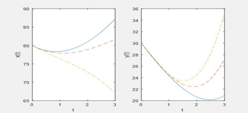
Figure 2. Plot for $L_i=\frac{d}{dt}$ when $p=0.7,q=0.9;$ solid line: $h_1=h_2=-1,$ dashed line: $h_1=-1.2,h_2=-1.2,$ dashed dotted line: $h_1=-1.4,h_2=-1.4.$

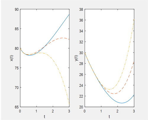
Figure 3. Plot for $L_1=D^p,L_2=D^q$ when $p=q=1;$ solid line: $h_1=h_2=-1,$ dashed line: $h_1=-1.2,h_2=-1.2,$ dashed dotted line: $h_1=-1.4,h_2=-1.4.$

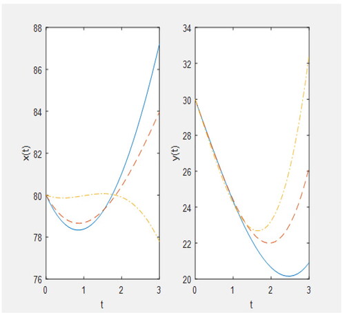
Figure 4. Plot for $L_1=D^p,L_2=D^q$ when $p=0.7,q=0.9;$ solid line: $h_1=h_2=-1,$ dashed line: $h_1=-1.2,h_2=-1.2,$ dashed dotted line: $h_1=-1.4,h_2=-1.4.$

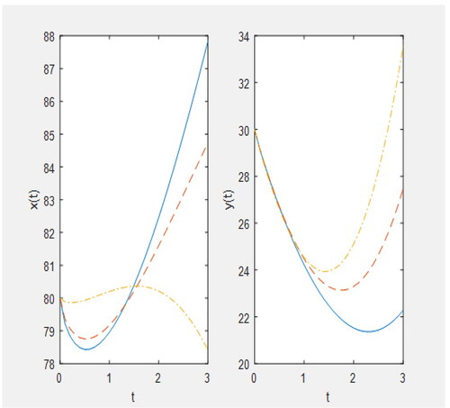
Figure 5. Plot for x(t) (i) for $L_1=\frac{d}{dt},$ (ii) for $L_1=D^p$ when $h_1=h_2=-1,q=0.9;$ solid line: p = 0.1, dashed line: p = 0.3, dashed dotted line: p = 0.5, dotted line: p = 0.7.

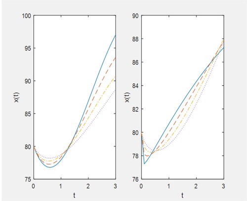
Figure 6. Plot for y(t) (i) for $L_2=\frac{d}{dt},$ (ii) for $L_2=D^q$ when $h_1=h_2=-1,p=0.7;$ solid line: q = 0.3, dashed line: q = 0.5, dashed dotted line: q = 0.7, dotted line: q = 0.9.

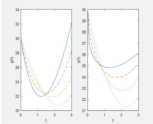
Figure 7. Plot for $L_1=D^p,L_2=D^q$ when $h_1=h_2=-1,q=0.9;$ solid line: p = 0.1, dashed line: p = 0.3, dashed dotted line: p = 0.5, dotted line: p = 0.7.

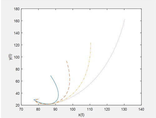
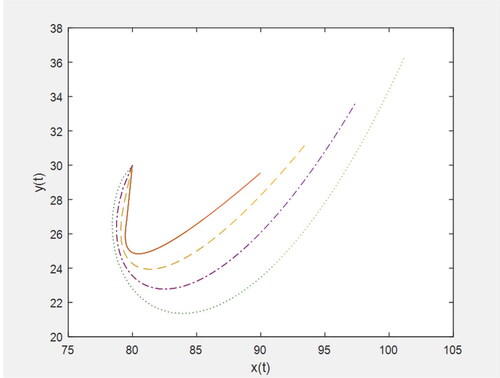
Figure 8. Plot for $L_1=D^p,L_2=D^q$ when $h_1=h_2=-1,p=0.7;$ solid line: q = 0.3, dashed line: q = 0.5, dashed dotted line: q = 0.7, dotted line: q = 0.9.

5. Concluding remark

1. Figures 1–2 and Figures 3–4 depict that for both the choices of auxiliary linear operators, decrease in the values of auxiliary parameters h₁ and h₂ shows the decay in mass concentration of prey species whereas that of predator shows a growth.

2. Figure 5 shows that for increase in the values of the fractional parameter p, prey population shows an increase for some time, although it decreases with time for different values of p but as the time goes on it shows the reverse trend i.e. greater values of p correspond to lesser values of prey population and it increases with the time t.

3. Figure 6 shows that for increase in the values of the fractional parameter q, predator population shows an increase for some time, although it decreases with time for different values of q but as the time goes on it shows the reverse trend i.e. greater values of q correspond to lesser values of predator population and it increases with the time t.

4. Figures 7 and 8 show the variation of predator population corresponding to the prey population for varying values of the fractional parameters p and q respectively.

5. These figures show that the mass concentration of prey increases and the same decreases for predator with the time t.

Authors’ contributions

The authors contributed equally and significantly in writing this paper. All authors read and approved the final manuscript.

Acknowledgements

The authors are grateful to the editor and reviewers for their thorough review and comments, which contributed to improving this article.

Disclosure statement

The authors declare that they have no competing interests.

References

- Abeye, N., Ayalew, M., Suthar, D. L., Purohit, S. D., & Jangid, K. (2022). Numerical solution of unsteady state fractional advection–dispersion equation. Arab Journal of Basic and Applied Sciences, 29(1), 77–85. doi:10.1080/25765299.2022.2064076
- Addison, L. M. (2017). Analysis of a predator-prey model: A deterministic and stochastic approach. Journal of Biometrics and Biostatistics, 8(4), 1–9.
- Agarwal, G., Yadav, L. K., Albalawi, W., Nisar, K. S., & Shefeeq, T. (2022). Two analytical approaches for space- and time-fractional coupled burger’s equations via Elzaki transform. Progress in Fractional Differentiation and Applications, 8, 177–190.
- Agarwal, R., Kritika, & Purohit, S. D. (2021). Mathematical model pertaining to the effect of buffer over cytosolic calcium concentration distribution. Chaos, Solitons & Fractals, 143, 110610. doi:10.1016/j.chaos.2020.110610
- Agarwal, R., Kritika, Purohit, S. D., & Kumar, D. (2021). Mathematical modelling of cytosolic calcium concentration distribution using non-local fractional operator. Discrete & Continuous Dynamical Systems, 14, 3387–3399.
- Alaria, A., Khan, A. M., Suthar, D. L., & Kumar, D. (2019). Application of fractional operators in modelling for charge carrier transport in amorphous semiconductor with multiple trapping. International Journal of Applied and Computational Mathematics, 5(6), 1–10. doi:10.1007/s40819-019-0750-8
- Anisiu, M. C. (2014). Lotka-Volterra and their model. Didatica Mathematica, 32, 9–17.
- Carmichael, R. D., & Lotka, A. J. (1926). Elements of physical biology. The American Mathematical Monthly, 33(8), 426–428. doi:10.2307/2298330
- Dave, S., Khan, A. M., Purohit, S. D., & Suthar, D. L. (2021). Application of green synthesized metal nano-particles in photo catalytic degradation of dyes and its mathematical modelling using Caputo Fabrizio fractional derivative without singular kernel. Journal of Mathematics, 2021, 1–8. doi:10.1155/2021/9948422
- Doungmo Goufo, E. F., Kumar, S., & Mugisha, S. B. (2020). Similarities in a fifth-order evolution equation with and with no singular kernel. Chaos, Solitons & Fractals, 130, 109467. doi:10.1016/j.chaos.2019.109467
- Ghanbari, B., Kumar, S., & Kumar, R. (2020). A study of behaviour for immune and tumor cells in immunogenetic tumour model with non-singular fractional derivative. Chaos, Solitons & Fractals, 133, 109619. doi:10.1016/j.chaos.2020.109619
- Hassani, M., Tabar, M. M., Nemati, H., Domairry, G., & Noori, F. (2011). An analytical solution for boundary layer flow of a nanofluid past a stretching sheet. International Journal of Thermal Sciences, 48, 1–8.
- Khan, A. M., Purohit, S. D., Dave, S., & Suthar, D. L. (2021). Fractional mathematical modelling of degradation of dye in textile effluents. Mathematics in Engineering, Science and Aerospace, 2021(3), 1–9.
- Kritika, R., & Agarwal, S. D. (2020). Mathematical model for anomalous subdiffusion using conformable operator. Chaos, Solitons & Fractals, 140, 110199. doi:10.1016/j.chaos.2020.110199
- Kumar, S., Kumar, R., Agarwal, R. P., & Samet, B. (2020). A study on fractional Lotka-Volterra population model using Haar wavelet and Adams-Bashforth-Moulton methods. Mathematical Methods in the Applied Sciences, 43(8), 5564–5578. doi:10.1002/mma.6297
- Kumar, S., Kumar, A., Samet, B., Gómez-Aguilar, J. F., & Osman, M. S. (2020). A chaos study of tumor and effector cells in fractional tumor-immune model for cancer treatment. Chaos, Solitons & Fractals, 141, 110321. doi:10.1016/j.chaos.2020.110321
- Liao, S. J. (1997). An approximate solution technique which does not depend upon small parameters: A special example. International Journal of Non-Linear Mechanics, 32(5), 815–822. doi:10.1016/S0020-7462(96)00101-1
- Liao, S. J. (2004). On the homotopy analysis method for nonlinear problems. Applied Mathematics and Computation, 147(2), 499–513. doi:10.1016/S0096-3003(02)00790-7
- Liu, X., & Chen, L. (2003). Complex dynamics of Holling type-II Lotka-Volterra predator-prey system with impulsive perturbations on the predator. Chaos, Solitons & Fractals, 16(2), 311–320. doi:10.1016/S0960-0779(02)00408-3
- Maiti, A., Sen, P., & Samanta, G. P. (2016). Deterministic and stochastic analysis of a prey-predator model with herd behavior in both Systems. Science & Control Engineering, 4(1), 259–269. doi:10.1080/21642583.2016.1241194
- Miller, K. S., & Ross, B. (1993). An introduction to the fractional calculus and fractional differential equations. New York: Wiley.
- Mistry, L., Khan, A. M., & Suthar, D. L. (2020). An epidemic slia mathematical model with Caputo Fabrizio Fractional derivative. Test Engineering and Management, 83, 26374–26391.
- Nassar, C. J., Revelli, J. F., & Bowman, R. J. (2011). Application of the homotopy analysis method to the Poisson-Boltzmann equation for semiconductor devices. International Journal of Nonlinear Sciences and Numerical Simulation, 16(6), 2501–2512. doi:10.1016/j.cnsns.2010.09.015
- Oldham, K. B., & Spanier, J. (1974). The fractional calculus. New York: Academic Press.
- Pareek, N., Gupta, A., Agarwal, G., & Suthar, D. L. (2021). Natural transform along with HPM technique for solving fractional ADE. Advances in Mathematical Physics, 2021, 1–11. doi:10.1155/2021/9915183
- Podlubny, I. (1999). Fractional differential equations. San Diego: Academic Press.
- Ramani, P., Khan, A. M., & Suthar, D. L. (2019). Revisiting analytical-approximate solution of time fractional Rosenau-Hyman equation via fractional reduced differential transform method. International Journal on Emerging Technologies, 10(2), 403–409.
- Ramani, P., Khan, A. M., Suthar, D. L., & Kumar, D. (2022). Approximate analytical solution for non-linear Fitzhugh–Nagumo equation of time fractional order through fractional reduced differential transform method. International Journal of Applied and Computational Mathematics, 8(2), 61. doi:10.1007/s40819-022-01254-z
- Song, L., & Zhang, H. (2007). Application of homotopy analysis method to fractional KdV Burgers-Kuramoto equation. Physics Letters A, 367(1–2), 88–94. doi:10.1016/j.physleta.2007.02.083
- Sprott, J. C., Wildenberg, J. C., & Azizi, Y. (2005). A simple spatiotemporal chaotic Lotka-Volterra Model. Chaos, Solitons & Fractals, 26(4), 1035–1043. doi:10.1016/j.chaos.2005.02.015
- Suthar, D. L., Purohit, S. D., & Araci, S. (2020). Solution of fractional kinetic equations associated with the (p, q)-Mathieu-type series. Discrete Dynamics in Nature and Society, 2020, 1–7. doi:10.1155/2020/8645161
- Tiwana, M. H., Maqbool, K., & Mann, A. B. (2017). Homotopy perturbation Laplace transform solution of fractional non-linear reaction diffusion system of Lotka-Volterra type differential Equation. Engineering Science and Technology, 20(2), 672–678. doi:10.1016/j.jestch.2016.10.014
- Veeresha, P., Prakasha, D. G., & Kumar, S. (2020). A fractional model for propagation of classical optical solitons by using nonsingular derivative. Mathematical Methods in the Applied Sciences, 1–15.
- Volterra, V. (1926). Fluctuations in the abundance of a species considered mathematically. Nature, 118(2972), 558–560. doi:10.1038/118558a0
- Wu, Y., Wang, C., & Liao, S. (2005). Solving the one loop solution of the Vakhnenko equation by means of the homotopy analysis. Chaos, Solitons & Fractals, 23(5), 1733–1740. doi:10.1016/S0960-0779(04)00437-0
- Xiao, D., & Ruan, S. (2001a). Codimension two bifurcations in a predator prey system with group defense. International Journal of Bifurcation and Chaos, 11(08), 2123–2131. doi:10.1142/S021812740100336X
- Xiao, D., & Ruan, S. (2001b). Global dynamics of a ratio-dependent predator-prey system. Journal of Mathematical Biology, 43(3), 268–290. doi:10.1007/s002850100097
- Yadav, L. K., Agarwal, G., Suthar, D. L., & Purohit, S. D. (2022). Time-fractional partial differential equations: A novel technique for analytical and numerical solutions. Arab Journal of Basic and Applied Sciences, 29(1), 86–98. doi:10.1080/25765299.2022.2064075
- Zurigat, M., Momani, S., Odibat, Z., & Alawneh, A. (2010). The homotopy analysis method for handling system of fractional differential equations. Applied Mathematical Modelling, 34(1), 24–35. doi:10.1016/j.apm.2009.03.024