On Maxwell–Lomax distribution: properties and applications

Abstract

The development of new generalizations based on certain baseline probability distribution has become one of the current trends in distribution theory literature. New generators are often required to define wider distributions for modelling real life data. In this study, we proposed and studied a new generalization of Maxwell and Lomax distributions using the T-X method. Several structural and statistical properties of the proposed distribution were obtained such as moments, quantile function, survival and hazard functions, skewness, kurtosis and order statistics. The method of maximum likelihood estimation (MLE) was used to estimate the parameters of the proposed distribution. In addition, a simulation study was conducted to evaluate the performance of the MLE method. The proposed distribution was applied to two real life datasets to illustrate its flexibility. It was found that the proposed distribution was superior to offer a better fit than the other competing extensions of Lomax distributions considered in the study.

Keywords:

• Hazard function
• Maxwell–Lomax
• moments
• order statistics
• quantile function

1. Introduction

Lomax distribution, pioneered by Lomax (1954) and described by Bryson (1974) is a heavy-tailed alternative to exponential, Weibull and gamma distributions and has been gaining popularity in distribution theory literature. Al-Zahrani and Al-Sobhi (2013) reported that the distribution had been widely applied in actuarial sciences, economics, demography, reliability engineering, biological sciences and many more. Some other important studies involving Lomax distribution and its variants include Salem (2014) who studied four methods of estimation of parameters of Lomax distribution. Cordeiro, Edwin, Ortega, and Popović (2015) investigated Gamma–Lomax distribution and studied its properties. Tahir, Cordeiro, Mansoor, and Zubair (2015) introduced Weibull–Lomax distribution with increasing and decreasing shapes for the hazard function. Mead (2016) proposed a five-parameter beta exponentiated Lomax distribution. Rady, Hassanein, and Elhaddad (2016) used a three-parameters Power Lomax distribution in modelling data on remission times of bladder cancer patients. Gompertz–Lomax distribution with increasing, decreasing and constant failure rate was applied by Oguntunde, Khaleel, Ahmed, Adejumo, and Odetunmibi (2017) to data relating to the strengths of 1.5 cm glass fibres. A study on application of Half-logistic-Lomax distribution to the data on bladder cancer patients was carried out by Anwar and Zahoor (2018). Park and Mahmoudi (2018) considered the problem of estimating parameters of Lomax distribution from fuzzy information.

A random variable X is said to have a Lomax distribution with parameters $\varpi =(\beta ,\theta )$ if the cumulative distribution function (cdf) and probability density function (pdf) are respectively given as (1) $$Q\left(x;\beta ,\theta \right)=1-{\left(1+\theta x\right)}^{-\beta },\theta ,\beta >0;x>0,$$(1) and (2) $$q\left(x;\beta ,\theta \right)=\beta \theta {\left(1+\theta x\right)}^{-\left(1+\beta \right)},\theta ,\beta >0;x>0,$$(2) where $\beta \mathrm{ }$and$\mathrm{ }\theta \mathrm{ }$are the shape and scale parameters, respectively.

1.1. Maxwell distribution

Maxwell distribution, introduced by Maxwell (1860) is a continuous distribution which is mostly used in the field of statistical mechanics to determine the speed of ideal gases (molecules). The distribution, characterized by a scale parameter λ is defined by the pdf (3) $$g(u,\lambda )=\sqrt{\frac{2}{\pi }}\frac{u^2{e}^{-\mathrm{ }\frac{u^2}{2{\lambda }^2}}}{{\lambda }^3},u,\lambda >0,$$(3) and cdf function given by (4) $$G(u,\lambda )=\frac{2}{\sqrt{\pi }}\gamma \left(\frac{3}{2},\frac{u^2}{2{\lambda }^2}\right),u,\lambda >0,$$(4) where $\gamma (a,z)={\int }_0^z{t}^{a-1}{e}^{-t}dt$denotes an incomplete gamma function.

Often times, due to limited range of behaviours, some commonly used distributions such as Lomax, Weibull, gamma and lognormal do not provide adequate fit to complex data sets in different areas of applications. Therefore, generalizing such distributions tends to offer more flexibility and provide reasonable parametric fits to the data sets.

In this study therefore, we have proposed a three-parameter continuous probability distribution, named Maxwell–Lomax (M–L) distribution that would be more flexible and improve the goodness-of-fit to real life data than the Lomax distribution.

The motivations of this study include obtaining a flexible distribution that are both right-skewed and left-skewed, deriving some statistical properties such as moments; quantile function; order statistics among others, estimating the parameters of the proposed M–L distribution using maximum likelihood method of estimation and illustrating the performance and potentiality of the proposed distribution against some competing distributions.

Several studies involving Maxwell distribution have been carried out in the recent past. Some of such studies are as follows: Shakil, Golam Kibria, and Singh (2006) derived the distributions of the ratio |X/Y| when X and Y are independently and identically distributed, Bayesian analysis of Maxwell distribution based on type I and reliability estimation of progressively type II censored data were discussed in Kazmi, Aslam, and Ali (2012) and Krishna and Malik (2012), Bayesian analysis of Maxwell distribution under different loss functions and prior distributions was studied in Dey, Dey, and Maiti (2013) and Al-Baldawi (2013), Li (2016) studied Minimax estimation of the Parameters of Maxwell distribution under different loss functions, Sharma, Dey, Singh, and Manzoor (2018) addressed the various properties and different methods of estimation of the unknown parameters of length and area-biased Maxwell distribution while Singh and Sharma (2019) introduced a location-scale family of Maxwell distribution for modelling the total annual rainfall of India from 1901 to 2014.

Despite the aforementioned studies on Maxwell distribution, only a few studies on its generalization exists in the literature. Some of such studies include Yuri, Juan, Heleno, and Hector (2016), who introduced Gamma–Maxwell distribution by applying Gamma-G family defined by Zografos and Balakrishnan (2009). Sharma, Bakouch, and Suthar (2017) proposed an extension of Maxwell distribution using the Maxwell-X family of distribution and Weibull distribution. Ishaq and Abiodun (2020a) proposed Maxwell–Weibull distribution by applying the odd ratio link approach of Alzaatreh, Lee, and Famoye (2013) and Almheidat, Lee, and Famoye (2016). Dagum distribution was generalized by Ishaq and Abiodun (2020b) in Maxwell-Dagum model framework. Abdullahi, Suleiman, Ishaq, Usman, and Suleiman (2021) proposed Maxwell-Exponential distribution, derived its properties and applied it to data on strengths of glass fibres. Bayesian estimation of the parameter of Maxwell–Mukherjee Islam distribution was obtained by Ishaq, Abiodun, and Falgore (2021). Ishaq and Abiodun (2021) proposed and studied Maxwell–Dagum distribution using maximum likelihood, maximum product of spacing, least squares and weighted least squares estimation methods.

The remaining part of this paper is organized as follows. Section 2 presents the cdf, pdf and linear representation of the M–L distribution. Some statistical properties including moment, survival function, hazard function, quantile function, skewness and kurtosis, and order statistics are provided in Sect. 3. Parameters estimates are derived and a simulation study conducted in Sect. 4, applications to real datasets are provided in Sect. 5 and the conclusion of the study is provided in Sect. 6.

2. Generalization of M–L distribution

Consider a random variable X with pdf q(x) and cdf Q(x). Let W be a continuous random variable with pdf p(w) defined on $\left[a,b\right],$ Alzaatreh et al. (2013) and Almheidat et al. (2016) defined the cdf of family of distributions as (5) $$F(x)={\int }_0^{\frac{Q(x)}{1-Q(x)}}p(w)dw, w\ge 0,$$(5) where $Q(x)$ is the cdf of any continuous random variable X. The generalization of Maxwell distribution referred to as Maxwell generalized family of distributions can be obtained by substituting the pdf in (3)(3) $$g(u,\lambda )=\sqrt{\frac{2}{\pi }}\frac{u^2{e}^{-\mathrm{ }\frac{u^2}{2{\lambda }^2}}}{{\lambda }^3},u,\lambda >0,$$(3) into (5)(5) $$F(x)={\int }_0^{\frac{Q(x)}{1-Q(x)}}p(w)dw, w\ge 0,$$(5) and replacing $Q(x)$ by $Q(x,\varpi )$ to obtain (6) $$F(x,\lambda ,\varpi )=\frac{2}{\sqrt{\pi }}\gamma \left(\frac{3}{2},\frac{1}{2{\lambda }^2}{\left(\frac{Q(x,\varpi )}{1-Q(x,x\varpi }\right)}^2\right),\lambda >0;\mathrm{ }x>0,$$(6) where $\varpi =(\beta ,\theta )$ denotes the parameters of the Lomax distribution and $\gamma (a,b)={\int }_0^a{s}^{b-1}{e}^{-s}ds$denotes the lower incomplete gamma function.

Substituting (1)(1) $$Q\left(x;\beta ,\theta \right)=1-{\left(1+\theta x\right)}^{-\beta },\theta ,\beta >0;x>0,$$(1) , with $Q(x,\varpi )=Q(x,\beta ,\theta )=1-{(1+\theta \mathrm{ }x)}^{-\beta },$ the cdf in (6)(6) $$F(x,\lambda ,\varpi )=\frac{2}{\sqrt{\pi }}\gamma \left(\frac{3}{2},\frac{1}{2{\lambda }^2}{\left(\frac{Q(x,\varpi )}{1-Q(x,x\varpi }\right)}^2\right),\lambda >0;\mathrm{ }x>0,$$(6) can be written as (7) $$F\left(x;\lambda ,\beta ,\theta \right)=F\left(x\right)=\frac{2}{\sqrt{\pi }}\gamma \left(\frac{3}{2},\frac{1}{2{\lambda }^2}{\left(\frac{1-{\left(1+\theta x\right)}^{-\beta }}{{\left(1+\theta x\right)}^{-\beta }}\right)}^2\right),\lambda ,\beta ,\theta ;x>0,$$(7) (8) $$=\frac{\gamma \left(a,w\right)}{\Gamma \left(a\right)},$$(8) where $a=\frac{3}{2}$ and $w=\frac{1}{2{\lambda }^2}{\left(\frac{1-{(1+\theta x)}^{-\beta }}{{(1+\theta x)}^{-\beta }}\right)}^2.$

The pdf can be obtained from (7)(7) $$F\left(x;\lambda ,\beta ,\theta \right)=F\left(x\right)=\frac{2}{\sqrt{\pi }}\gamma \left(\frac{3}{2},\frac{1}{2{\lambda }^2}{\left(\frac{1-{\left(1+\theta x\right)}^{-\beta }}{{\left(1+\theta x\right)}^{-\beta }}\right)}^2\right),\lambda ,\beta ,\theta ;x>0,$$(7) by applying the differentiation approach as in Gradshteyn and Ryzhik (2000) and Ishaq and Abiodun (2020a, 2020b), which gives (9) $$f(x,\lambda ,\varpi )=\frac{2q(x,\varpi )}{{\lambda }^3\sqrt{2\pi {(1-Q(x,\varpi \left)\right)}^2}}{\left(\frac{Q(x,\varpi )}{(1-Q(x,\varpi \left)\right)}\right)}^2\hspace{0.17em}\text{exp}\hspace{0.17em}\left(-\frac{1}{2{\lambda }^2}{\left(\frac{Q(x,\varpi )}{(1-Q(x,\varpi \left)\right)}\right)}^2\right),\mathrm{ }\mathrm{ }\lambda >0;x>0.$$(9)

Also, using (1)(1) $$Q\left(x;\beta ,\theta \right)=1-{\left(1+\theta x\right)}^{-\beta },\theta ,\beta >0;x>0,$$(1) and (2)(2) $$q\left(x;\beta ,\theta \right)=\beta \theta {\left(1+\theta x\right)}^{-\left(1+\beta \right)},\theta ,\beta >0;x>0,$$(2) , the pdf in (9)(9) $$f(x,\lambda ,\varpi )=\frac{2q(x,\varpi )}{{\lambda }^3\sqrt{2\pi {(1-Q(x,\varpi \left)\right)}^2}}{\left(\frac{Q(x,\varpi )}{(1-Q(x,\varpi \left)\right)}\right)}^2\hspace{0.17em}\text{exp}\hspace{0.17em}\left(-\frac{1}{2{\lambda }^2}{\left(\frac{Q(x,\varpi )}{(1-Q(x,\varpi \left)\right)}\right)}^2\right),\mathrm{ }\mathrm{ }\lambda >0;x>0.$$(9) can be written as (10) $$f\left(x;\lambda ,\beta ,\theta \right)=f\left(x\right)=\frac{2\beta \theta {\left(1+\theta x\right)}^{-\left(1+\beta \right)}}{{\lambda }^3\sqrt{2\pi }{\left({\left(1+\theta x\right)}^{-\beta }\right)}^2}{\left(\frac{1-{\left(1+\theta x\right)}^{-\beta }}{{\left(1+\theta x\right)}^{-\beta }}\right)}^2\hspace{0.17em}\text{exp}\hspace{0.17em}\left(-\frac{1}{2{\lambda }^2}{\left(\frac{1-{\left(1+\theta x\right)}^{-\beta }}{{\left(1+\theta x\right)}^{-\beta }}\right)}^2\right),\lambda ,\beta ,\theta ;x>0.$$(10)

2.1. Linear representations for the M–L distribution

Consider the exponential series expansion given by (11) $$e^{-x}=\sum _{l=0}^{\infty }\frac{{\left(-1\right)}^l}{l}{x}^l$$(11)

By applying (11)(11) $$e^{-x}=\sum _{l=0}^{\infty }\frac{{\left(-1\right)}^l}{l}{x}^l$$(11) on the pdf in (10)(10) $$f\left(x;\lambda ,\beta ,\theta \right)=f\left(x\right)=\frac{2\beta \theta {\left(1+\theta x\right)}^{-\left(1+\beta \right)}}{{\lambda }^3\sqrt{2\pi }{\left({\left(1+\theta x\right)}^{-\beta }\right)}^2}{\left(\frac{1-{\left(1+\theta x\right)}^{-\beta }}{{\left(1+\theta x\right)}^{-\beta }}\right)}^2\hspace{0.17em}\text{exp}\hspace{0.17em}\left(-\frac{1}{2{\lambda }^2}{\left(\frac{1-{\left(1+\theta x\right)}^{-\beta }}{{\left(1+\theta x\right)}^{-\beta }}\right)}^2\right),\lambda ,\beta ,\theta ;x>0.$$(10) , we obtain (12) $$\begin{array}{c}f\left(x\right)=\frac{2\beta \theta {\left(1+\theta x\right)}^{-\left(1+\beta \right)}}{{\lambda }^3\sqrt{2\pi }{\left({\left(1+\theta x\right)}^{-\beta }\right)}^2}\sum _{l=0}^{\infty }\frac{{\left(-1\right)}^l}{l!{\left(2{\lambda }^2\right)}^l}{\left(\frac{1-{\left(1+\theta x\right)}^{-\beta }}{{\left(1+\theta x\right)}^{-\beta }}\right)}^{2+2l}\\ =\frac{2\beta \theta {\left(1+\theta x\right)}^{-\left(1+\beta \right)}}{{\lambda }^3\sqrt{2\pi }}\sum _{l=0}^{\infty }\frac{{\left(-1\right)}^l}{l!{\left(2{\lambda }^2\right)}^l}\frac{{\left(1-{\left(1+\theta x\right)}^{-\beta }\right)}^{2+2l}}{{\left({\left(1+\theta x\right)}^{-\beta }\right)}^{4+2l}}\end{array}$$(12)

The denominator of the last term of (12)(12) $$\begin{array}{c}f\left(x\right)=\frac{2\beta \theta {\left(1+\theta x\right)}^{-\left(1+\beta \right)}}{{\lambda }^3\sqrt{2\pi }{\left({\left(1+\theta x\right)}^{-\beta }\right)}^2}\sum _{l=0}^{\infty }\frac{{\left(-1\right)}^l}{l!{\left(2{\lambda }^2\right)}^l}{\left(\frac{1-{\left(1+\theta x\right)}^{-\beta }}{{\left(1+\theta x\right)}^{-\beta }}\right)}^{2+2l}\\ =\frac{2\beta \theta {\left(1+\theta x\right)}^{-\left(1+\beta \right)}}{{\lambda }^3\sqrt{2\pi }}\sum _{l=0}^{\infty }\frac{{\left(-1\right)}^l}{l!{\left(2{\lambda }^2\right)}^l}\frac{{\left(1-{\left(1+\theta x\right)}^{-\beta }\right)}^{2+2l}}{{\left({\left(1+\theta x\right)}^{-\beta }\right)}^{4+2l}}\end{array}$$(12) can be written as ${(1-(1-{(1+\theta x)}^{-\beta }))}^{4+2l}.$ Therefore, for $n>0$ and $\left|z\right|<1,$ the generalized binomial expansion can be obtained as (13) $${\left(1-z\right)}^{-n}=\sum _{m=0}^{\infty }\frac{\Gamma \left(n+m\right)}{m!\Gamma \left(n\right)}{z}^m.$$(13)

By applying (13)(13) $${\left(1-z\right)}^{-n}=\sum _{m=0}^{\infty }\frac{\Gamma \left(n+m\right)}{m!\Gamma \left(n\right)}{z}^m.$$(13) to the denominator of (12)(12) $$\begin{array}{c}f\left(x\right)=\frac{2\beta \theta {\left(1+\theta x\right)}^{-\left(1+\beta \right)}}{{\lambda }^3\sqrt{2\pi }{\left({\left(1+\theta x\right)}^{-\beta }\right)}^2}\sum _{l=0}^{\infty }\frac{{\left(-1\right)}^l}{l!{\left(2{\lambda }^2\right)}^l}{\left(\frac{1-{\left(1+\theta x\right)}^{-\beta }}{{\left(1+\theta x\right)}^{-\beta }}\right)}^{2+2l}\\ =\frac{2\beta \theta {\left(1+\theta x\right)}^{-\left(1+\beta \right)}}{{\lambda }^3\sqrt{2\pi }}\sum _{l=0}^{\infty }\frac{{\left(-1\right)}^l}{l!{\left(2{\lambda }^2\right)}^l}\frac{{\left(1-{\left(1+\theta x\right)}^{-\beta }\right)}^{2+2l}}{{\left({\left(1+\theta x\right)}^{-\beta }\right)}^{4+2l}}\end{array}$$(12) we can write (14) $$f\left(x\right)=\frac{2\beta \theta {\left(1+\theta x\right)}^{-\left(1+\beta \right)}}{{\lambda }^3\sqrt{2\pi }}\sum _{l,m=0}^{\infty }\frac{{\left(-1\right)}^l\Gamma \left(4+2l+m\right)}{{\left(2{\lambda }^2\right)}^{l}l!m!\Gamma \left(4+2l\right)}{\left(1-{\left(1+\theta x\right)}^{-\beta }\right)}^{2+2l+m}.$$(14)

Also consider the expansion (15) $${\left(1-x\right)}^n=\sum _{v=0}^{\infty }{\left(-1\right)}^v\left(\underset{v}{\overset{n}{}}\right)x^v.$$(15)

Using (15)(15) $${\left(1-x\right)}^n=\sum _{v=0}^{\infty }{\left(-1\right)}^v\left(\underset{v}{\overset{n}{}}\right)x^v.$$(15) , the pdf in (14)(14) $$f\left(x\right)=\frac{2\beta \theta {\left(1+\theta x\right)}^{-\left(1+\beta \right)}}{{\lambda }^3\sqrt{2\pi }}\sum _{l,m=0}^{\infty }\frac{{\left(-1\right)}^l\Gamma \left(4+2l+m\right)}{{\left(2{\lambda }^2\right)}^{l}l!m!\Gamma \left(4+2l\right)}{\left(1-{\left(1+\theta x\right)}^{-\beta }\right)}^{2+2l+m}.$$(14) can be written as (16) $$\begin{array}{c}f\left(x\right)=\frac{2\beta \theta }{{\lambda }^3\sqrt{2\pi }}\sum _{l,m,v=0}^{\infty }\frac{{\left(-1\right)}^{l+v}\Gamma \left(4+2l+m\right)}{{\left(2{\lambda }^2\right)}^{l}l!m!\Gamma \left(4+2l\right)}\left(\underset{v}{\overset{2+2l+m}{}}\right){\left(1+\theta x\right)}^{-\left(1+\beta +\beta v\right)}\\ =\sum _{l,m,v=0}^{\infty }{\Omega }_{l,m,v}{\left(1+\theta x\right)}^{-\left(1+\beta +\beta v\right)}\end{array}$$(16)

The expression in (16)(16) $$\begin{array}{c}f\left(x\right)=\frac{2\beta \theta }{{\lambda }^3\sqrt{2\pi }}\sum _{l,m,v=0}^{\infty }\frac{{\left(-1\right)}^{l+v}\Gamma \left(4+2l+m\right)}{{\left(2{\lambda }^2\right)}^{l}l!m!\Gamma \left(4+2l\right)}\left(\underset{v}{\overset{2+2l+m}{}}\right){\left(1+\theta x\right)}^{-\left(1+\beta +\beta v\right)}\\ =\sum _{l,m,v=0}^{\infty }{\Omega }_{l,m,v}{\left(1+\theta x\right)}^{-\left(1+\beta +\beta v\right)}\end{array}$$(16) is the pdf of M–L distribution expressed as a linear representation of exponentiated-G density defined by Gupta, Gupta, and Gupta (1998), where $${\Omega }_{l,m,v}=\frac{2\beta \theta }{{\lambda }^3\sqrt{2\pi }}\frac{{\left(-1\right)}^{l+v}\Gamma \left(4+2l+m\right)}{{\left(2{\lambda }^2\right)}^{l}l!m!\Gamma \left(4+2l\right)}\left(\underset{v}{\overset{2+2l+m}{}}\right).$$

Plots of the pdf of M–L distribution for different parameter values are displayed in Figure 1(a) and (b), respectively

Figure 1. Plots of pdf of M–L distribution.

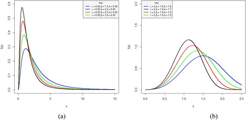
As observed, the plots of the pdf show (a) left-skewed and (b) right-skewed distributions for the various parameter values. This indicates that the proposed distribution can be used to model both left and right-skewed data sets.

3. Statistical properties of M–L distribution

Some statistical properties of the proposed M–L distribution are discussed in this section. These include moments, quantile function, survival function, hazard function, skewness and kurtosis, and order statistics.

3.1. Moments

The $r^{th}$ moment $(r=1,2,...)$ of a random variable $X$is defined as (17) $$E(X^r)=\underset{-\infty }{\overset{\infty }{\int }}{x}^{r}f\left(x\right)dx$$(17)

Let the pdf $f(x)$ be as defined (16)(16) $$\begin{array}{c}f\left(x\right)=\frac{2\beta \theta }{{\lambda }^3\sqrt{2\pi }}\sum _{l,m,v=0}^{\infty }\frac{{\left(-1\right)}^{l+v}\Gamma \left(4+2l+m\right)}{{\left(2{\lambda }^2\right)}^{l}l!m!\Gamma \left(4+2l\right)}\left(\underset{v}{\overset{2+2l+m}{}}\right){\left(1+\theta x\right)}^{-\left(1+\beta +\beta v\right)}\\ =\sum _{l,m,v=0}^{\infty }{\Omega }_{l,m,v}{\left(1+\theta x\right)}^{-\left(1+\beta +\beta v\right)}\end{array}$$(16) , then the moments of the M–L distribution is obtained as (18) $$E(X^r)=\sum _{l,m,v=0}^{\infty }{\Omega }_{l,m,v}\underset{0}{\overset{\infty }{\int }}{x}^r{\left(1+\theta x\right)}^{-\left(1+\beta +\beta v\right)}dx.$$(18)

If we let (19) $$A=\theta x,\Rightarrow x=\frac{A}{\theta },dx=\frac{dA}{\theta },$$(19) then inserting (19)(19) $$A=\theta x,\Rightarrow x=\frac{A}{\theta },dx=\frac{dA}{\theta },$$(19) into (18)(18) $$E(X^r)=\sum _{l,m,v=0}^{\infty }{\Omega }_{l,m,v}\underset{0}{\overset{\infty }{\int }}{x}^r{\left(1+\theta x\right)}^{-\left(1+\beta +\beta v\right)}dx.$$(18) gives (20) $$E(X^r)=\frac{1}{{\theta }^{1+r}}\sum _{l,m,v=0}^{\infty }{\Omega }_{l,m,v}\underset{0}{\overset{\infty }{\int }}{A}^r{\left(1+A\right)}^{-\left(1+\beta +\beta v\right)}dA.$$(20)

Also, let (21) $$1+A=\frac{1}{Z},\Rightarrow A=\frac{1-Z}{Z},dA=\frac{-dZ}{Z^2}.$$(21)

Substituting (21)(21) $$1+A=\frac{1}{Z},\Rightarrow A=\frac{1-Z}{Z},dA=\frac{-dZ}{Z^2}.$$(21) into (20)(20) $$E(X^r)=\frac{1}{{\theta }^{1+r}}\sum _{l,m,v=0}^{\infty }{\Omega }_{l,m,v}\underset{0}{\overset{\infty }{\int }}{A}^r{\left(1+A\right)}^{-\left(1+\beta +\beta v\right)}dA.$$(20) gives (22) $$\begin{array}{c}E(X^r)=\frac{1}{{\theta }^{1+r}}\sum _{l,m,v=0}^{\infty }{\Omega }_{l,m,v}\underset{0}{\overset{1}{\int }}{Z}^{\beta \left(1+v\right)-r-1}{\left(1-Z\right)}^{(r+1)-1}dZ\\ =\frac{1}{{\theta }^{1+r}}\sum _{l,m,v=0}^{\infty }{\Omega }_{l,m,v}B\left(r+1,\beta \left(1+v\right)-r\right).\end{array}$$(22)

For $r=1,2,...,k,$ (22)(22) $$\begin{array}{c}E(X^r)=\frac{1}{{\theta }^{1+r}}\sum _{l,m,v=0}^{\infty }{\Omega }_{l,m,v}\underset{0}{\overset{1}{\int }}{Z}^{\beta \left(1+v\right)-r-1}{\left(1-Z\right)}^{(r+1)-1}dZ\\ =\frac{1}{{\theta }^{1+r}}\sum _{l,m,v=0}^{\infty }{\Omega }_{l,m,v}B\left(r+1,\beta \left(1+v\right)-r\right).\end{array}$$(22) gives the mean (1st moment), 2nd moment, …., kth moment respectively of the M–L distribution.

3.2. Survival and hazard functions

Survival function, denoted $S(x),$ is the probability that an individual survives longer than a particular time x (Lee & Wang, 2003). The survival function of M–L distribution is given by: (23) $$S(x)=1-F(x)=1-\frac{2}{\sqrt{\pi }}\gamma \left(\frac{3}{2},\frac{1}{2{\lambda }^2}{\left(\frac{1-{\left(1+\theta x\right)}^{-\beta }}{{\left(1+\theta x\right)}^{-\beta }}\right)}^2\right),\lambda ,\beta ,\theta ;x>0,$$(23) where $F(x)$ is as defined in (7)(7) $$F\left(x;\lambda ,\beta ,\theta \right)=F\left(x\right)=\frac{2}{\sqrt{\pi }}\gamma \left(\frac{3}{2},\frac{1}{2{\lambda }^2}{\left(\frac{1-{\left(1+\theta x\right)}^{-\beta }}{{\left(1+\theta x\right)}^{-\beta }}\right)}^2\right),\lambda ,\beta ,\theta ;x>0,$$(7) .

The hazard function is mathematically obtained as the ratio of the density function to the survival function. Thus, from the pdf in (10)(10) $$f\left(x;\lambda ,\beta ,\theta \right)=f\left(x\right)=\frac{2\beta \theta {\left(1+\theta x\right)}^{-\left(1+\beta \right)}}{{\lambda }^3\sqrt{2\pi }{\left({\left(1+\theta x\right)}^{-\beta }\right)}^2}{\left(\frac{1-{\left(1+\theta x\right)}^{-\beta }}{{\left(1+\theta x\right)}^{-\beta }}\right)}^2\hspace{0.17em}\text{exp}\hspace{0.17em}\left(-\frac{1}{2{\lambda }^2}{\left(\frac{1-{\left(1+\theta x\right)}^{-\beta }}{{\left(1+\theta x\right)}^{-\beta }}\right)}^2\right),\lambda ,\beta ,\theta ;x>0.$$(10) and the survival function in (23)(23) $$S(x)=1-F(x)=1-\frac{2}{\sqrt{\pi }}\gamma \left(\frac{3}{2},\frac{1}{2{\lambda }^2}{\left(\frac{1-{\left(1+\theta x\right)}^{-\beta }}{{\left(1+\theta x\right)}^{-\beta }}\right)}^2\right),\lambda ,\beta ,\theta ;x>0,$$(23) , the hazard function of M–L distribution can be obtained as (24) $$h\left(x\right)=\frac{f(x)}{S(x)}=\frac{2\beta \theta {\left(1+\theta x\right)}^{3\beta -1}{\left(1-{\left(1+\theta x\right)}^{-\beta }\right)}^2\hspace{0.17em}\text{exp}\hspace{0.17em}\left(-\frac{1}{2{\lambda }^2}{\left(\frac{1-{\left(1+\theta x\right)}^{-\beta }}{{\left(1+\theta x\right)}^{-\beta }}\right)}^2\right)}{{\lambda }^3\sqrt{2\pi }\left\{1-\frac{2}{\sqrt{\pi }}\gamma \left(\frac{3}{2},\frac{1}{2{\lambda }^2}{\left(\frac{1-{\left(1+\theta x\right)}^{-\beta }}{{\left(1+\theta x\right)}^{-\beta }}\right)}^2\right)\right\}},\lambda ,\beta ,\theta ;x>0.$$(24)

The plots of hazard function of M-L distribution for different parameter values are displayed in Figure 2(a) and (b), respectively.

Figure 2. Plots of hazard function of M–L distribution.

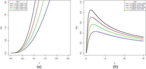
As seen from Figure 2, the hazard plots of the M-L distribution have (a) increasing and (b) upside-down bathtub.

3.3. Quantile function

Quantiles are more useful measures in descriptive statistics than the mean because they are less susceptible to long-tailed distributions (Rady et al., 2016).

Let X denote a random variable with the M–L cdf given in (7)(7) $$F\left(x;\lambda ,\beta ,\theta \right)=F\left(x\right)=\frac{2}{\sqrt{\pi }}\gamma \left(\frac{3}{2},\frac{1}{2{\lambda }^2}{\left(\frac{1-{\left(1+\theta x\right)}^{-\beta }}{{\left(1+\theta x\right)}^{-\beta }}\right)}^2\right),\lambda ,\beta ,\theta ;x>0,$$(7) . Following the method in Oluyede (2018), the quantile function can be obtained by inverting the cdf in (8)(8) $$=\frac{\gamma \left(a,w\right)}{\Gamma \left(a\right)},$$(8) as (25) $$w={\gamma }^{-1}\left(a,u\Gamma \left(a\right)\right)$$(25)

By substituting for $a$ and $w$ using (8)(8) $$=\frac{\gamma \left(a,w\right)}{\Gamma \left(a\right)},$$(8) , Eq. (25)(25) $$w={\gamma }^{-1}\left(a,u\Gamma \left(a\right)\right)$$(25) becomes (26) $${\left(\frac{1-{\left(1+\theta x\right)}^{-\beta }}{{\left(1+\theta x\right)}^{-\beta }}\right)}^2=2{\lambda }^2{\gamma }^{-1}\left(\frac{3}{2},u\Gamma \left(\frac{3}{2}\right)\right).$$(26)

Taking the square root of both sides and simplifying gives (27) $$1={\left(1+\theta x\right)}^{-\beta }\left[1+{\left\{2{\lambda }^2{\gamma }^{-1}\left(\frac{3}{2},u\Gamma \left(\frac{3}{2}\right)\right)\right\}}^{\frac{1}{2}}\right],$$(27) from which (28) $$1+\theta x={\left[1+{\left\{2{\lambda }^2{\gamma }^{-1}\left(\frac{3}{2},u\Gamma \left(\frac{3}{2}\right)\right)\right\}}^{\frac{1}{2}}\right]}^{\frac{1}{\beta }}.$$(28)

Therefore, the quantile function $x=Q(u)=F^{-1}(u)$ of the M–L distribution can be obtained from (28) as (29) $$x=Q(u)={\theta }^{-1}\left\{1+{\left[{\left\{2{\lambda }^2{\gamma }^{-1}\left(\frac{3}{2},u\Gamma \left(\frac{3}{2}\right)\right)\right\}}^{\frac{1}{2}}\right]}^{\frac{1}{\beta }}-1\right\},$$(29) where $u$is a uniform distribution on interval (0, 1).

The second quartile which is the median of M-L can be obtained from (29)(29) $$x=Q(u)={\theta }^{-1}\left\{1+{\left[{\left\{2{\lambda }^2{\gamma }^{-1}\left(\frac{3}{2},u\Gamma \left(\frac{3}{2}\right)\right)\right\}}^{\frac{1}{2}}\right]}^{\frac{1}{\beta }}-1\right\},$$(29) by letting $u=\frac{1}{2}.$

3.4. Skewness and kurtosis

The skewness can be used to measure asymmetry of probability distribution, that is how a distribution deviates from normal distribution while kurtosis can be used to measure whether or not a probability distribution is light or heavy-tailed relative to the normal distribution. Classical measures of skewness and kurtosis do not exist in some applications. This article thus presents the Bowley skewness (SK) given by (30) $$SK=\frac{Q\left(\frac{3}{4}\right)-2Q\left(\frac{1}{2}\right)+Q\left(\frac{1}{4}\right)}{Q\left(\frac{3}{4}\right)-Q\left(\frac{1}{4}\right)}$$(30) and the Moors (1988) kurtosis (KT) given by (31) $$KT=\frac{Q\left(\frac{7}{8}\right)-Q\left(\frac{5}{8}\right)-Q\left(\frac{3}{8}\right)+Q\left(\frac{1}{8}\right)}{Q\left(\frac{6}{8}\right)-Q\left(\frac{2}{8}\right)}$$(31) where $Q(.)$ denotes the quantile function obtained from (29)(29) $$x=Q(u)={\theta }^{-1}\left\{1+{\left[{\left\{2{\lambda }^2{\gamma }^{-1}\left(\frac{3}{2},u\Gamma \left(\frac{3}{2}\right)\right)\right\}}^{\frac{1}{2}}\right]}^{\frac{1}{\beta }}-1\right\},$$(29) .

The values of the quantiles as well as skewness and kurtosis of M-L distribution for some parameters values $\lambda ,\theta ,\beta$ are presented in Tables 1 and 2.

Table 1. Skewness and Kurtosis results of the M–L distribution setting $\mathrm{\lambda }$= 0.05 and θ = 0.05.

$Q(.)$	β = 1.5	β = 2.5	β = 3.5	β = 4.5	β = 5.5
¼	0.7275	0.4334	0.3086	0.2396	0.1958
½	1.0127	0.6016	0.4279	0.3320	0.2713
¾	1.3294	0.7874	0.5593	0.4337	0.3541
1/8	0.5509	0.3288	0.2343	0.1820	0.1488
2/8	0.7275	0.4334	0.3086	0.2396	0.1958
3/8	0.8735	0.5196	0.3698	0.2870	0.2345
5/8	1.1590	0.6876	0.4887	0.3791	0.3096
6/8	1.3294	0.7874	0.5593	0.4337	0.3541
7/8	1.5668	0.9259	0.6571	0.5092	0.4157
Skewness	0.0523	0.0494	0.0482	0.0475	0.0471
Kurtosis	0.1417	0.1342	0.1310	0.1292	0.1281

Table 2. Skewness and Kurtosis results of the M–L distribution setting $\mathrm{\lambda }$=5 and θ = 1.6.

$Q(.)$	β = 1.9	β = 2.9	β = 3.9	β = 4.9	β = 5.9
¼	1.0497	0.5671	0.3852	0.2909	0.2335
½	1.3254	0.6923	0.4631	0.3467	0.2767
¾	1.5971	0.8098	0.5345	0.3971	0.3153
1/8	0.8574	0.4756	0.3270	0.2486	0.2004
2/8	1.0497	0.5671	0.3852	0.2909	0.2335
3/8	1.1952	0.6340	0.4271	0.3210	0.2568
5/8	1.4546	0.7489	0.4976	0.3712	0.2955
6/8	1.5971	0.8098	0.5345	0.3971	0.3153
7/8	1.7837	0.8877	0.5809	0.4296	0.3401
Skewness	−0.0074	−0.0317	−0.0435	−0.0505	−0.0551
Kurtosis	−0.0158	−0.0808	−0.1127	−0.1317	−0.1443

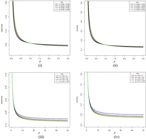
As observed from Table 1, for fixed parameters $\lambda =0.05$ and $\theta =0.05,$the value of skewness decreases with increase in the value of parameter $\beta ,$ and M–L distribution shows a slightly positive skewness (right skewness). Also, from Table 2, fixing parameters $\lambda =5$ and $\theta =1.6,$the value of skewness decreases with increase in the value of parameter$\beta ,$ and M–L distribution shows a slightly negative skewness (left skewness). The kurtosis as shown in the two tables are platykurtic since the computed values are less than 3 for all parameter values considered. Figure 3 displays the skewness and kurtosis plots of M–L distribution as a function of β, which shows their variability for different values of $\theta$ and $\lambda .$

Figure 3. Plots of skewness and kurtosis of M–L distribution for different parameter values.

3.5. Order statistics

Let X₁, X₂,…,X_n denote the random sample from M–L random variables, and X₍₁₎, X₍₂₎,…,X_(n)denote the order statistics of the sample. The density function of the ith orderstatistics X_(i), denoted $f_{i,n}(x)$) for $i=1,2,...,n$ is given by (32) $$f_{i,n}(x)=\frac{n!}{\left(i-1\right)!\left(n-i\right)!}f(x)F{(x)}^{i-1}{\left[1-F(x)\right]}^{n-i},$$(32) where $F(x)$ and $f(x)$ are the cdf and pdf defined in (7)(7) $$F\left(x;\lambda ,\beta ,\theta \right)=F\left(x\right)=\frac{2}{\sqrt{\pi }}\gamma \left(\frac{3}{2},\frac{1}{2{\lambda }^2}{\left(\frac{1-{\left(1+\theta x\right)}^{-\beta }}{{\left(1+\theta x\right)}^{-\beta }}\right)}^2\right),\lambda ,\beta ,\theta ;x>0,$$(7) and (10)(10) $$f\left(x;\lambda ,\beta ,\theta \right)=f\left(x\right)=\frac{2\beta \theta {\left(1+\theta x\right)}^{-\left(1+\beta \right)}}{{\lambda }^3\sqrt{2\pi }{\left({\left(1+\theta x\right)}^{-\beta }\right)}^2}{\left(\frac{1-{\left(1+\theta x\right)}^{-\beta }}{{\left(1+\theta x\right)}^{-\beta }}\right)}^2\hspace{0.17em}\text{exp}\hspace{0.17em}\left(-\frac{1}{2{\lambda }^2}{\left(\frac{1-{\left(1+\theta x\right)}^{-\beta }}{{\left(1+\theta x\right)}^{-\beta }}\right)}^2\right),\lambda ,\beta ,\theta ;x>0.$$(10) , respectively. Using the expansion in (15)(15) $${\left(1-x\right)}^n=\sum _{v=0}^{\infty }{\left(-1\right)}^v\left(\underset{v}{\overset{n}{}}\right)x^v.$$(15) , the ith order statistics in (32)(32) $$f_{i,n}(x)=\frac{n!}{\left(i-1\right)!\left(n-i\right)!}f(x)F{(x)}^{i-1}{\left[1-F(x)\right]}^{n-i},$$(32) can be written as (33) $$f_{i,n}(x)=\frac{n!f(x)}{\left(i-1\right)!\left(n-i\right)!}\sum _{j=0}^{\infty }{\left(-1\right)}^j\left(\underset{j}{\overset{{}^{{}^{n-i}}}{}}\right)F{(x)}^{i+j-1}.$$(33)

Inserting (7)(7) $$F\left(x;\lambda ,\beta ,\theta \right)=F\left(x\right)=\frac{2}{\sqrt{\pi }}\gamma \left(\frac{3}{2},\frac{1}{2{\lambda }^2}{\left(\frac{1-{\left(1+\theta x\right)}^{-\beta }}{{\left(1+\theta x\right)}^{-\beta }}\right)}^2\right),\lambda ,\beta ,\theta ;x>0,$$(7) into (33)(33) $$f_{i,n}(x)=\frac{n!f(x)}{\left(i-1\right)!\left(n-i\right)!}\sum _{j=0}^{\infty }{\left(-1\right)}^j\left(\underset{j}{\overset{{}^{{}^{n-i}}}{}}\right)F{(x)}^{i+j-1}.$$(33) becomes (34) $$f_{i,n}(x)=\frac{n!f(x)}{\left(i-1\right)!\left(n-i\right)!}\sum _{j=0}^{\infty }{\left(-1\right)}^j\left(\underset{j}{\overset{{}^{{}^{n-i}}}{}}\right){\left[{\gamma }_1\left(a,w\right)\right]}^{i+j-1},$$(34) where ${\gamma }_1(a,w)=\frac{\gamma (a,w)}{\Gamma (a)},$ $a=\frac{3}{2}$ and $w=\frac{1}{2{\lambda }^2}{\left(\frac{1-{(1+\theta x)}^{-\beta }}{{(1+\theta x)}^{-\beta }}\right)}^2.$

By applying (15)(15) $${\left(1-x\right)}^n=\sum _{v=0}^{\infty }{\left(-1\right)}^v\left(\underset{v}{\overset{n}{}}\right)x^v.$$(15) , the last term of (34)(34) $$f_{i,n}(x)=\frac{n!f(x)}{\left(i-1\right)!\left(n-i\right)!}\sum _{j=0}^{\infty }{\left(-1\right)}^j\left(\underset{j}{\overset{{}^{{}^{n-i}}}{}}\right){\left[{\gamma }_1\left(a,w\right)\right]}^{i+j-1},$$(34) yields (35) $$f_{i,n}(x)=\frac{n!f(x)}{\left(i-1\right)!\left(n-i\right)!}\sum _{j=0}^{\infty }{\left(-1\right)}^j\left(\underset{j}{\overset{{}^{{}^{n-i}}}{}}\right)\sum _{k=0}^{\infty }\sum _{q=0}^k{\left(-1\right)}^{k+q}\left(\underset{k}{\overset{i+j-1}{}}\right)\left(\underset{q}{\overset{{}^k}{}}\right){\left[{\gamma }_1\left(a,w\right)\right]}^q.$$(35)

Finally, (35)(35) $$f_{i,n}(x)=\frac{n!f(x)}{\left(i-1\right)!\left(n-i\right)!}\sum _{j=0}^{\infty }{\left(-1\right)}^j\left(\underset{j}{\overset{{}^{{}^{n-i}}}{}}\right)\sum _{k=0}^{\infty }\sum _{q=0}^k{\left(-1\right)}^{k+q}\left(\underset{k}{\overset{i+j-1}{}}\right)\left(\underset{q}{\overset{{}^k}{}}\right){\left[{\gamma }_1\left(a,w\right)\right]}^q.$$(35) can be expressed as (36) $$f_{i,n}(x)=\Phi f(x)\sum _{q=0}^{\infty }{\left[{\gamma }_1\left(a,w\right)\right]}^q$$(36) where $\Phi =\frac{n!}{(i-1)!(n-i)!}{\sum }_{j=0}^{\infty }{\sum }_{k=q}^{\infty }{(-1)}^{j+k+q}\left(\underset{j}{\overset{n-i}{}}\right)\left(\underset{k}{\overset{i+j-1}{}}\right)\left(\underset{q}{\overset{k}{}}\right).$

As given in Gradshteyn and Ryzhik (2000), the power series expansion for the ratio of incomplete gamma function in (36)(36) $$f_{i,n}(x)=\Phi f(x)\sum _{q=0}^{\infty }{\left[{\gamma }_1\left(a,w\right)\right]}^q$$(36) is given by (37) $${\gamma }_1{}^q\left(a,w\right)=\frac{w^{aq}}{{\left[\Gamma \left(a\right)\right]}^q}\sum _{\tau =0}^{\infty }{A}_{q,\tau }{w}^{\tau },q\ge 1,$$(37) where $A_{q,\tau }={(\tau c_0)}^{-1}{\sum }_{p=1}^{\tau }(qp-\tau +p)c_p{A}_{q,\tau -p}$ with $c_p={(-1)}^p/p!(a+p).$

By substituting (37)(37) $${\gamma }_1{}^q\left(a,w\right)=\frac{w^{aq}}{{\left[\Gamma \left(a\right)\right]}^q}\sum _{\tau =0}^{\infty }{A}_{q,\tau }{w}^{\tau },q\ge 1,$$(37) into (36)(36) $$f_{i,n}(x)=\Phi f(x)\sum _{q=0}^{\infty }{\left[{\gamma }_1\left(a,w\right)\right]}^q$$(36) we get (38) $$\begin{array}{c}{f}_{i,n}(x)=\Phi f(x)\sum _{q,\tau =0}^{\infty }\frac{A_{q,\tau }}{{\left[\Gamma \left(a\right)\right]}^q}{w}^{\tau +aq}\\ =\Phi f(x)\sum _{q,\tau =0}^{\infty }\frac{A_{q,\tau }}{{\left[\Gamma \left(\frac{3}{2}\right)\right]}^q{\left(2{\lambda }^2\right)}^{\frac{2\tau +3q}{2}}}{\left(\frac{1-{\left(1+\theta x\right)}^{-\beta }}{{\left(1+\theta x\right)}^{-\beta }}\right)}^{2\tau +3q}\end{array}.$$(38)

Replacing $f(x)$ in (38)(38) $$\begin{array}{c}{f}_{i,n}(x)=\Phi f(x)\sum _{q,\tau =0}^{\infty }\frac{A_{q,\tau }}{{\left[\Gamma \left(a\right)\right]}^q}{w}^{\tau +aq}\\ =\Phi f(x)\sum _{q,\tau =0}^{\infty }\frac{A_{q,\tau }}{{\left[\Gamma \left(\frac{3}{2}\right)\right]}^q{\left(2{\lambda }^2\right)}^{\frac{2\tau +3q}{2}}}{\left(\frac{1-{\left(1+\theta x\right)}^{-\beta }}{{\left(1+\theta x\right)}^{-\beta }}\right)}^{2\tau +3q}\end{array}.$$(38) with the pdf in (12)(12) $$\begin{array}{c}f\left(x\right)=\frac{2\beta \theta {\left(1+\theta x\right)}^{-\left(1+\beta \right)}}{{\lambda }^3\sqrt{2\pi }{\left({\left(1+\theta x\right)}^{-\beta }\right)}^2}\sum _{l=0}^{\infty }\frac{{\left(-1\right)}^l}{l!{\left(2{\lambda }^2\right)}^l}{\left(\frac{1-{\left(1+\theta x\right)}^{-\beta }}{{\left(1+\theta x\right)}^{-\beta }}\right)}^{2+2l}\\ =\frac{2\beta \theta {\left(1+\theta x\right)}^{-\left(1+\beta \right)}}{{\lambda }^3\sqrt{2\pi }}\sum _{l=0}^{\infty }\frac{{\left(-1\right)}^l}{l!{\left(2{\lambda }^2\right)}^l}\frac{{\left(1-{\left(1+\theta x\right)}^{-\beta }\right)}^{2+2l}}{{\left({\left(1+\theta x\right)}^{-\beta }\right)}^{4+2l}}\end{array}$$(12) , we get (39) $$f_{i,n}(x)=\frac{2\Phi \beta \theta {\left(1+\theta x\right)}^{-\left(1+\beta \right)}}{{\lambda }^3\sqrt{2\pi }}\sum _{q,\tau ,l=0}^{\infty }\frac{{\left(-1\right)}^l{A}_{q,\tau }}{l!{\left[\Gamma \left(\frac{3}{2}\right)\right]}^q{\left(2{\lambda }^2\right)}^{l+\frac{2\tau +3q}{2}}}\frac{{\left(1-{\left(1+\theta x\right)}^{-\beta }\right)}^{2+2l+2\tau +3q}}{{\left({\left(1+\theta x\right)}^{-\beta }\right)}^{4+2l+2\tau +3q}}.$$(39)

Using (13)(13) $${\left(1-z\right)}^{-n}=\sum _{m=0}^{\infty }\frac{\Gamma \left(n+m\right)}{m!\Gamma \left(n\right)}{z}^m.$$(13) , the pdf in (39)(39) $$f_{i,n}(x)=\frac{2\Phi \beta \theta {\left(1+\theta x\right)}^{-\left(1+\beta \right)}}{{\lambda }^3\sqrt{2\pi }}\sum _{q,\tau ,l=0}^{\infty }\frac{{\left(-1\right)}^l{A}_{q,\tau }}{l!{\left[\Gamma \left(\frac{3}{2}\right)\right]}^q{\left(2{\lambda }^2\right)}^{l+\frac{2\tau +3q}{2}}}\frac{{\left(1-{\left(1+\theta x\right)}^{-\beta }\right)}^{2+2l+2\tau +3q}}{{\left({\left(1+\theta x\right)}^{-\beta }\right)}^{4+2l+2\tau +3q}}.$$(39) becomes (40) $$f_{i,n}(x)={\left(1+\theta x\right)}^{-\left(1+\beta \right)}\sum _{q,\tau ,l,m=0}^{\infty }{\Lambda }_{q,\tau ,l,m}{\left(1-{\left(1+\theta x\right)}^{-\beta }\right)}^{2+2l+2\tau +3q+m},$$(40) where ${\Lambda }_{q,\tau ,l,m}=\frac{2\Phi \beta \theta {(-1)}^l{A}_{q,\tau }\Gamma (4+2l+2\tau +3q+m)}{{\lambda }^3\sqrt{2\pi }l!m!{\left[\Gamma (\frac{3}{2})\right]}^q{(2{\lambda }^2)}^{l+\frac{2\tau +3q}{2}}\Gamma (4+2l+2\tau +3q)}.$

By applying the expansion in (15)(15) $${\left(1-x\right)}^n=\sum _{v=0}^{\infty }{\left(-1\right)}^v\left(\underset{v}{\overset{n}{}}\right)x^v.$$(15) , we can write (40)(40) $$f_{i,n}(x)={\left(1+\theta x\right)}^{-\left(1+\beta \right)}\sum _{q,\tau ,l,m=0}^{\infty }{\Lambda }_{q,\tau ,l,m}{\left(1-{\left(1+\theta x\right)}^{-\beta }\right)}^{2+2l+2\tau +3q+m},$$(40) as the ith order statistics expressed in terms of exponentiated-G density given by $$f_{i,n}(x)=\sum _{v=0}^{\infty }{\Psi }_v{\left(1+\theta x\right)}^{-\beta }{}^{\left(1+v\right)-1},$$ where (41) $${\Psi }_v=\sum _{q,\tau ,l,m=0}^{\infty }{\Lambda }_{q,\tau ,l,m}{\left(-1\right)}^v\left(\underset{v}{\overset{2+2l+2\tau +3q+m}{}}\right).$$(41)

The mean of order statistics is defined as (42) $$E(X)=\underset{-\infty }{\overset{\infty }{\int }}x{f}_{i,n}\left(x\right)dx,$$(42) where $f_{i,n}(x)$ is as given in (41)(41) $${\Psi }_v=\sum _{q,\tau ,l,m=0}^{\infty }{\Lambda }_{q,\tau ,l,m}{\left(-1\right)}^v\left(\underset{v}{\overset{2+2l+2\tau +3q+m}{}}\right).$$(41) .

Therefore, using (41)(41) $${\Psi }_v=\sum _{q,\tau ,l,m=0}^{\infty }{\Lambda }_{q,\tau ,l,m}{\left(-1\right)}^v\left(\underset{v}{\overset{2+2l+2\tau +3q+m}{}}\right).$$(41) , the mean of order statistics of the M–L distribution can be written as (43) $$E(X)=\sum _{v=0}^{\infty }{\Psi }_v\underset{0}{\overset{\infty }{\int }}x{\left(1+\theta x\right)}^{-\beta }{}^{\left(1+v\right)-1}dx$$(43)

By applying (19)(19) $$A=\theta x,\Rightarrow x=\frac{A}{\theta },dx=\frac{dA}{\theta },$$(19) , Eq. (43)(43) $$E(X)=\sum _{v=0}^{\infty }{\Psi }_v\underset{0}{\overset{\infty }{\int }}x{\left(1+\theta x\right)}^{-\beta }{}^{\left(1+v\right)-1}dx$$(43) can be expressed as (44) $$E(X)=\frac{1}{{\theta }^2}\sum _{v=0}^{\infty }{\Psi }_v\underset{0}{\overset{\infty }{\int }}A{\left(1+A\right)}^{-\beta }{}^{\left(1+v\right)-1}dA$$(44)

We can express (39)(39) $$f_{i,n}(x)=\frac{2\Phi \beta \theta {\left(1+\theta x\right)}^{-\left(1+\beta \right)}}{{\lambda }^3\sqrt{2\pi }}\sum _{q,\tau ,l=0}^{\infty }\frac{{\left(-1\right)}^l{A}_{q,\tau }}{l!{\left[\Gamma \left(\frac{3}{2}\right)\right]}^q{\left(2{\lambda }^2\right)}^{l+\frac{2\tau +3q}{2}}}\frac{{\left(1-{\left(1+\theta x\right)}^{-\beta }\right)}^{2+2l+2\tau +3q}}{{\left({\left(1+\theta x\right)}^{-\beta }\right)}^{4+2l+2\tau +3q}}.$$(39) by applying (21)(21) $$1+A=\frac{1}{Z},\Rightarrow A=\frac{1-Z}{Z},dA=\frac{-dZ}{Z^2}.$$(21) as (45) $$\begin{array}{c}E(X)=\frac{1}{{\theta }^2}\sum _{v=0}^{\infty }{\Psi }_v\underset{0}{\overset{1}{\int }}{Z}^{\beta }{}^{\left(1+v\right)-1-1}{\left(1-Z\right)}^{2-1}dZ\\ =\frac{1}{{\theta }^2}\sum _{v=0}^{\infty }{\Psi }_{v}B\left(2,\beta \left(1+v\right)-1\right)\end{array}$$(45)

4. Maximum likelihood estimation of parameters

In this section, we obtain the maximum likelihood estimates (MLEs) of the parameters of M–L distribution. Let X₁, X₂, …, X_n be the random sample from M–L distribution with parameter vector $(\Omega =\lambda ,\beta ,\theta ).$ The likelihood function is given by (46) $$\begin{array}{c}\ell \left(x_i/\Omega \right)=\prod _{i=1}^{n}f\left(x_i,\Omega \right)\\ ={\left(\frac{2\beta \theta }{{\lambda }^3\sqrt{2\pi }}\right)}^n\prod _{i=1}^n{\left(1+\theta x_i\right)}^{\beta -1}{\left(\frac{1-{\left(1+\theta x_i\right)}^{-\beta }}{{\left(1+\theta x_i\right)}^{-\beta }}\right)}^2\hspace{0.17em}\text{exp}\hspace{0.17em}\left(-\frac{1}{2{\lambda }^2}{\left(\frac{1-{\left(1+\theta x_i\right)}^{-\beta }}{{\left(1+\theta x_i\right)}^{-\beta }}\right)}^2\right),\end{array}$$(46) and the log-likelihood function $\ell (\Omega )$ is (47) $$\begin{array}{c}\ell =\ell (\Omega )=n\hspace{0.17em}\text{log}\hspace{0.17em}(2)+n\hspace{0.17em}\text{log}\hspace{0.17em}(\beta )+n\hspace{0.17em}\text{log}\hspace{0.17em}(\theta )-3n\hspace{0.17em}\text{log}\hspace{0.17em}(\lambda )-\frac{n}{2}\text{log}\hspace{0.17em}(2\pi )+(\beta -1)\sum _{i=1}^n\hspace{0.17em}\text{log}\hspace{0.17em}(1+\theta \mathrm{ }{x}_i)\\ +2\sum _{i=1}^n\hspace{0.17em}\text{log}\hspace{0.17em}\left(\frac{1-{(1+\theta \mathrm{ }{x}_i)}^{-\beta }}{{(1+\theta \mathrm{ }{x}_i)}^{-\beta }}\right)-\frac{1}{2{\lambda }^2}{\sum _{i=1}^n\left(\frac{1-{(1+\theta \mathrm{ }{x}_i)}^{-\beta }}{{(1+\theta \mathrm{ }{x}_i)}^{-\beta }}\right)}^2\end{array}.$$(47)

Calculating the first-order partial derivatives of (47)(47) $$\begin{array}{c}\ell =\ell (\Omega )=n\hspace{0.17em}\text{log}\hspace{0.17em}(2)+n\hspace{0.17em}\text{log}\hspace{0.17em}(\beta )+n\hspace{0.17em}\text{log}\hspace{0.17em}(\theta )-3n\hspace{0.17em}\text{log}\hspace{0.17em}(\lambda )-\frac{n}{2}\text{log}\hspace{0.17em}(2\pi )+(\beta -1)\sum _{i=1}^n\hspace{0.17em}\text{log}\hspace{0.17em}(1+\theta \mathrm{ }{x}_i)\\ +2\sum _{i=1}^n\hspace{0.17em}\text{log}\hspace{0.17em}\left(\frac{1-{(1+\theta \mathrm{ }{x}_i)}^{-\beta }}{{(1+\theta \mathrm{ }{x}_i)}^{-\beta }}\right)-\frac{1}{2{\lambda }^2}{\sum _{i=1}^n\left(\frac{1-{(1+\theta \mathrm{ }{x}_i)}^{-\beta }}{{(1+\theta \mathrm{ }{x}_i)}^{-\beta }}\right)}^2\end{array}.$$(47) with respect to $\lambda ,$β, $\theta$ and equating to zero, we get the following nonlinear equations: (48) $$\frac{\partial \ell }{\partial \lambda }=\frac{-3n}{\lambda }+\frac{1}{{\lambda }^3}{\sum _{i=1}^n\left(\frac{1-m_i{}^{-\beta }}{m_i{}^{-\beta }}\right)}^2=0,$$(48) (49) $$\frac{\partial \ell }{\partial \beta }=\frac{n}{\beta }+\sum _{i=1}^n\hspace{0.17em}\text{log}\hspace{0.17em}(m_i)+\frac{1}{{\lambda }^2}\sum _{i=1}^n\left(\frac{\hspace{0.17em}\text{log}\hspace{0.17em}(m_i)}{m_i^{-\beta }}\right)\left[\left(\frac{1-m_i^{-\beta }}{m_i^{-\beta }}\right)-2{\lambda }^2\left(\frac{m_i^{-\beta }}{1-m_i^{-\beta }}\right)\right]=0,$$(49) (50) $$\frac{\partial \ell }{\partial \theta }=\frac{n}{\theta }+(\beta -1)\sum _{i=1}^n{x}_i(m_i^{-1})+\frac{2\beta }{{\lambda }^2}\sum _{i=1}^n(x_i{m}_i^{\beta -1})\left[{\lambda }^2\left(\frac{m_i^{-\beta }}{1-m_i^{-\beta }}\right)-\frac{1}{2}\left(\frac{1-m_i^{-\beta }}{m_i^{-\beta }}\right)\right]=0,$$(50) where $m_i=1+\theta \mathrm{ }{x}_i.$

Solving the nonlinear equations (48) (49)(49) $$\frac{\partial \ell }{\partial \beta }=\frac{n}{\beta }+\sum _{i=1}^n\hspace{0.17em}\text{log}\hspace{0.17em}(m_i)+\frac{1}{{\lambda }^2}\sum _{i=1}^n\left(\frac{\hspace{0.17em}\text{log}\hspace{0.17em}(m_i)}{m_i^{-\beta }}\right)\left[\left(\frac{1-m_i^{-\beta }}{m_i^{-\beta }}\right)-2{\lambda }^2\left(\frac{m_i^{-\beta }}{1-m_i^{-\beta }}\right)\right]=0,$$(49) and (50)(50) $$\frac{\partial \ell }{\partial \theta }=\frac{n}{\theta }+(\beta -1)\sum _{i=1}^n{x}_i(m_i^{-1})+\frac{2\beta }{{\lambda }^2}\sum _{i=1}^n(x_i{m}_i^{\beta -1})\left[{\lambda }^2\left(\frac{m_i^{-\beta }}{1-m_i^{-\beta }}\right)-\frac{1}{2}\left(\frac{1-m_i^{-\beta }}{m_i^{-\beta }}\right)\right]=0,$$(50) simultaneously gives the MLEs $\widehat{\lambda },\widehat{\beta }\mathrm{ }\text{and}\mathrm{ }\widehat{\theta },$ respectively. However, there is no closed form solution for these equations and the estimates cannot be obtained analytically. We have to use a numerical technique with the aid of suitable statistical software R to obtain the estimates.

4.1. Simulation study

A simulation study was carried out in this section in order to assess the performance of the MLEs of M–L distribution. This was carried out based on the quantile function defined in (29)(29) $$x=Q(u)={\theta }^{-1}\left\{1+{\left[{\left\{2{\lambda }^2{\gamma }^{-1}\left(\frac{3}{2},u\Gamma \left(\frac{3}{2}\right)\right)\right\}}^{\frac{1}{2}}\right]}^{\frac{1}{\beta }}-1\right\},$$(29) for two sets of parameter vector $\Omega =(\lambda ,\beta ,\theta ).$ Data were generated for sample sizes n = 10, 20, 30, 50, 100 and 200. The maximum likelihood estimates $\widehat{\lambda },\widehat{\beta }\mathrm{ }\text{and}\mathrm{ }\widehat{\theta }$ were determined based on each generated sample by maximizing the log-likelihood function in (47)(47) $$\begin{array}{c}\ell =\ell (\Omega )=n\hspace{0.17em}\text{log}\hspace{0.17em}(2)+n\hspace{0.17em}\text{log}\hspace{0.17em}(\beta )+n\hspace{0.17em}\text{log}\hspace{0.17em}(\theta )-3n\hspace{0.17em}\text{log}\hspace{0.17em}(\lambda )-\frac{n}{2}\text{log}\hspace{0.17em}(2\pi )+(\beta -1)\sum _{i=1}^n\hspace{0.17em}\text{log}\hspace{0.17em}(1+\theta \mathrm{ }{x}_i)\\ +2\sum _{i=1}^n\hspace{0.17em}\text{log}\hspace{0.17em}\left(\frac{1-{(1+\theta \mathrm{ }{x}_i)}^{-\beta }}{{(1+\theta \mathrm{ }{x}_i)}^{-\beta }}\right)-\frac{1}{2{\lambda }^2}{\sum _{i=1}^n\left(\frac{1-{(1+\theta \mathrm{ }{x}_i)}^{-\beta }}{{(1+\theta \mathrm{ }{x}_i)}^{-\beta }}\right)}^2\end{array}.$$(47) . The average estimates, average bias, denoted Bias and average mean square error denoted MSE were then determined from N = 1000 repetitions. Tables 3 and 4 show the results for parameter settings $\Omega =(\lambda ,\beta ,\theta )$ = (0.05, 1.5, 0.05) and (5, 1.9, 1.6), respectively.

Table 3. Simulation results of the M–L distribution setting $\lambda =0.05,$$\beta =1.5$ and $\theta =0.05.$

Parameter	n	Estimate ($\widehat{\Omega }$)	Bias	MSE
	10	0.3689	0.3189	0.7535
	20	0.2359	0.1858	0.5403
$\lambda$= 0.05	30	0.1580	0.1080	0.4329
	50	0.1265	0.0765	0.3925
	100	0.0649	0.0149	0.3182
	200	0.0514	0.0014	0.3020
	10	6.0617	4.5617	25.6208
	20	5.5131	4.0131	20.3680
$\beta$= 1.5	30	4.0720	2.5720	9.4371
	50	3.4164	1.9164	5.8389
	100	2.0230	0.5230	1.0465
	200	1.6140	0.1140	0.3769
	10	0.1429	0.0929	0.3515
	20	0.1187	0.0687	0.3234
$\theta$= 0.05	30	0.1033	0.0533	0.3061
	50	0.0936	0.0436	0.2955
	100	0.0637	0.0137	0.2638
	200	0.0526	0.0026	0.2526

Table 4. Simulation results of the M–L distribution setting $\lambda =5,$$\beta =1.9$ and $\theta =0.05.$

Parameter	n	Estimate ($\widehat{\Omega }$)	Bias	MSE
	10	10.2406	5.2406	32.9544
	20	9.5269	4.5269	25.2697
$\lambda$= 5	30	7.7501	2.7501	10.5631
	50	6.8224	1.8224	5.3935
	100	6.2875	1.2875	3.1951
	200	5.0802	0.0802	0.3366
	10	6.1413	4.2413	22.4799
	20	4.9038	3.0038	12.2766
$\beta$= 1.9	30	4.2645	2.3645	8.2053
	50	3.4131	1.5131	4.0525
	100	2.6180	0.7180	1.4835
	200	1.9083	0.0083	0.2583
	10	3.0858	1.4858	3.9434
	20	2.5877	0.9877	2.2132
$\theta$= 1.6	30	2.2882	0.6882	1.4118
	50	2.1716	0.5716	1.1483
	100	1.8564	0.2564	0.5721
	200	1.7072	0.1072	0.3686

It is observed from Tables 3 and 4 that as the sample size increases, the mean estimates of all the parameters approach true fixed values $\lambda =0.05,$ $\beta =1.5,$ $\theta =0.05,$ and $\lambda =5,$ $\beta =1.9,$ $\theta =1.6$ for Tables 3 and 4, respectively. Also, the estimates of the Bias and MSE decrease as the sample size increases,

5. Data application

Application of the M–L distribution to two real life datasets are provided to illustrate its potentiality empirically. Comparison of the proposed distribution is done with three other competing distributions, namely: Exponentiated-Lomax (E-L), Marshall Olkin-Lomax (MO-L) and Rayleigh-Lomax (R-L) distributions. The choice of the most appropriate distribution is based on the values of the likelihood-based statistics including Akaike's Information Criterion (AIC), Consistent Akaike's Information Criterion (CAIC), Bayesian Information Criterion (BIC), Hannan-Quinn Information Criterion (HQIC). These statistics are computed as follows $$\mathit{AIC}=-2\ell +2p,$$ $$\mathit{CAIC}=-2\ell +\frac{2np}{n-p-1},$$ $$\mathit{BIC}=-2\ell +p\hspace{0.17em}\text{log}(n),$$ $$\mathit{HQIC}=-2\ell +2p\hspace{0.17em}\text{log}(\text{log}\hspace{0.17em}(n),$$ where $\ell$ is the maximized log-likelihood of the parameter vector $\Omega =(\lambda ,\beta ,\theta ),$ n is the number of observations and$p$ is the number of estimated parameters.

We also compute Anderson-Darling $(A^{*})$ and Cramér-von Mises $(W^{*})$ statistics $$A^{*}=\left(\frac{9}{4n^2}+\frac{3}{4n}+1\right)\left\{n+\frac{1}{n}\sum _{j=1}^n(2j-1)\hspace{0.17em}\text{log}[z_i(1-z_{n-j+1})]\right\},$$ $$W^{*}=\left(\frac{1}{2n}+1\right)\left\{\sum _{j=1}^n{\left(z_i-\frac{2j-1}{2n}\right)}^2+\frac{1}{2n}\right\},$$ where $z_i=F(x_i)$ and are the ordered observations. The model with the smallest values of these statistics is preferred.

5.1. Dataset 1

This dataset relates to the total milk production in the first birth of 107 cows from SINDI race. The data- set can be found in Nasiru, Abubakari, and Angbing (2021), and is presented in the Appendix.

Descriptive statistics for dataset 1

Table

Sample size (n)	107
Mean	0.4689
Standard Deviation	0.1920
Minimum	0.0168
Maximum	0.8781
Skewness	−0.3353
Kurtosis	2.6861

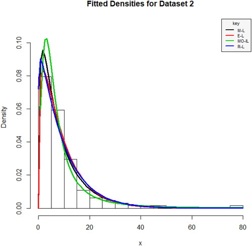
5.2. Dataset 2

The dataset consists of 128 random samples of the remission times (in months) of bladder cancer patients presented in Lee and Wang (2003). See the Appendix.

Descriptive statistics for dataset 2

Table

Sample size (n)	128
Mean	9.366
Standard Deviation	10.5083
Minimum	0.080
Maximum	79.050
Skewness	3.2866
Kurtosis	18.4831

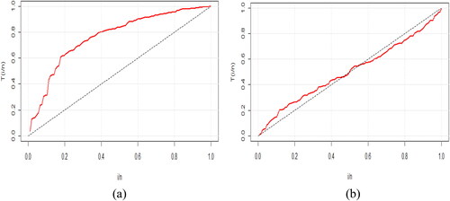
As observed from the descriptive statistics, dataset 1 is negatively skewed and platykurtic since the computed skewness is negative and kurtosis value is less than 3. For the dataset 2, the data is positively skewed and leptokurtic in terms of kurtosis. The total time on test (TTT) curves are plotted in Figure 4 to show the empirical behaviours of the hazard rate of the datasets. The concave nature of TTT plot for dataset 1 in (a) is an indication of increasing hazard rate while (b) shows that the shape of the hazard rate of dataset 2 is bathtub.

Figure 4. TTT plots of dataset 1 (a) dataset 2 (b).

Figures 5 and 6 display the densities plots of the M–L distribution against its competing distributions using dataset 1 and 2. It is observed from the figures that the datasets appear to follow the M–L distribution more reasonably well when compared to the other competing distributions.

Figure 5. Fitted densities of dataset 1.

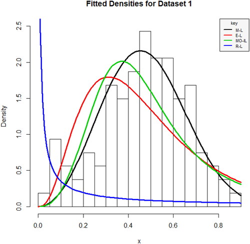
Figure 6. Fitted densities of dataset 2.

The numerical results for datasets 1 and 2 are presented in Tables 5 and 6, respectively, showing the maximum likelihood estimates (MLEs), standard error (sd), $\ell ,$ $\mathit{AIC},$ $\mathit{CAIC},$ $\mathit{BIC},$ $\mathit{HQIC},$ $A^{*}$ and $W^{*}$statistics. As observed from the tables, the M-L distribution provides the highest value of $\ell$ and lowest values of $\mathit{AIC},$ $\mathit{CAIC},$ $\mathit{BIC},$ $\mathit{HQIC},$ $A^{*}$ and $W^{*}$statistics than the competing distributions, indicating that M-L provides the best fit for the datasets.

Table 5. MLEs and Goodness-of-fit-statistics for dataset 1.

	M-L		E-L		MO-L		R-L
	Estimate	SE	Estimate	SE	Estimate	SE	Estimate	SE
$\widehat{\lambda }$	0.1986	0.1493	3.7420	0.5713	0.3200	0.0400	1.7512	0.3871
$\widehat{\theta }$	0.0270	0.0194	0.0061	0.0006	9.7630	0.2963	0.0021	0.0003
$\widehat{\beta }$	21.2522	9.5270	63.9000	29.9100	3.4350	0.1377	0.0804	0.0105
$\ell$	19.1700		4.9673		2.7547		−244.4227
$\mathit{AIC}$	−32.3400		−3.9347		0.4906		494.8454
$\mathit{CAIC}$	−32.1070		−3.7016		0.7236		495.0784
$\mathit{BIC}$	−24.3216		4.0838		8.5091		502.8639
$\mathit{HQIC}$	−29.0895		−0.6841		3.7412		498.0960
$A^{*}$	1.5819		6.0008		6.8619		2.0899
$W^{*}$	0.2412		1.0318		1.1895		0.3148

Table 6. MLEs and goodness-of-fit-statistics for dataset 2.

	M-L			E-L				MO-L		R-L
	Estimate		SE	Estimate		SE		Estimate	SE	Estimate		SE
$\widehat{\lambda }$	3.2684		1.0278	1.2200		0.1497		0.0024	0.0012	70.6600		3.8390
$\widehat{\theta }$	24.4847		8.8895	0.4321		0.0195		172.6000	14.4320	0.0015		0.0009
$\widehat{\beta }$	0.3550		0.0370	10.0000		4.2040		1.7860	0.1378	0.5238		0.0349
$\ell$		−411.5780			−413.0452		−412.3371				−414.1033
AIC		829.1560			832.0904		830.6742				834.2066
CAIC		829.3495			832.2839		830.8677				834.4001
BIC		837.7121			840.6465		839.2303				842.7627
HQIC		832.6324			835.5668		834.1506				837.6830
$A^{*}$		0.4028			0.5418		1.1898				1.4101
$W^{*}$		0.0586			0.0775		0.1788				0.2279

6. Conclusion

A three-parameter distribution was proposed in this study which compounded Maxwell generalized family and Lomax distributions. Some statistical properties of the distribution including moments, quantile function, survival function, hazard function, skewness, kurtosis and order statistics were studied. Maximum likelihood estimation method was used to estimate the parameters. A simulation study was carried out to illustrate the performances of the MLEs for different parameter values and sample sizes. Applications to two real life datasets were given to illustrate the flexibility and potentiality of the M–L distribution in comparison to some other existing distributions using $\mathit{AIC},$ $\mathit{CAIC},$ $\mathit{BIC},$ $\mathit{HQIC},$ $A^{*}$ and $W^{*}$criteria. The proposed distribution was found to provide a better fit to the two real life datasets with small number of observations that are positively and negatively skewed when compared with some other extensions of Lomax distribution including Exponentiated-Lomax, Marshall-Olkin-Lomax and Rayleigh-Lomax distributions, and therefore, could be an alternative for data modelling.

Authors’ contributions

The authors have equally contributed to this work. All authors read and approved the final manuscript.

Acknowledgments

The authors are grateful to the anonymous reviewers for their valuable comments and suggestions which greatly improved the quality of the article.

Disclosure Statement

The authors declare that they have no conflicts of interest.

Appendix

Dataset 1

0.4365, 0.4260, 0.5140, 0.6907, 0.7471, 0.2605, 0.6196, 0.8781, 0.4990, 0.6058, 0.6891, 0.5770, 0.5394, 0.1479, 0.2356, 0.6012, 0.1525, 0.5483, 0.6927, 0.7261, 0.3323, 0.0671, 0.2361, 0.4800, 0.5707, 0.7131, 0.5853, 0.6768, 0.5350, 0.4151, 0.6789, 0.4576, 0.3259, 0.2303, 0.7687, 0.4371, 0.3383, 0.6114, 0.3480, 0.4564, 0.7804, 0.3406, 0.4823, 0.5912, 0.5744, 0.5481, 0.1131, 0.7290, 0.0168, 0.5529, 0.4530, 0.3891, 0.4752, 0.3134, 0.3175, 0.1167, 0.6750, 0.5113, 0.5447, 0.4143, 0.5627, 0.5150, 0.0776, 0.3945, 0.4553, 0.4470, 0.5285, 0.5232, 0.6465, 0.0650, 0.8492, 0.8147, 0.3627, 0.3906, 0.4438, 0.4612, 0.3188, 0.2160, 0.6707, 0.6220, 0.5629, 0.4675, 0.6844, 0.3413, 0.4332, 0.0854, 0.3821, 0.4694, 0.3635, 0.4111, 0.5349, 0.3751, 0.1546, 0.4517, 0.2681, 0.4049, 0.5553, 0.5878, 0.4741, 0.3598, 0.7629, 0.5941, 0.6174, 0.6860, 0.0609, 0.6488, 0.2747.

Dataset 2

0.08, 2.09, 3.48,4.87, 6.94, 8.66, 13.11, 23.63, 0.20, 2.23, 3.52, 4.98, 6.97, 9.02, 13.29, 0.40, 2.26, 3.57,5.06, 7.09, 9.22, 13.80, 25.74, 0.50, 2.46, 3.64, 5.09, 7.26, 9.47, 14.24, 25.82, 0.51, 2.54,3.70, 5.17, 7.28, 9.74, 14.76, 26.31, 0.81, 2.62, 3.82, 5.32, 7.32, 10.06, 14.77, 32.15, 2.64,3.88, 5.32, 7.39, 10.34, 14.83, 34.26, 0.90, 2.69, 4.18, 5.34, 7.59, 10.66, 15.96, 36.66, 1.05,2.69, 4.23, 5.41, 7.62, 10.75, 16.62, 43.01, 1.19, 2.75, 4.26, 5.41, 7.63, 17.12, 46.12, 1.26,2.83, 4.33, 5.49, 7.66, 11.25, 17.14, 79.05, 1.35, 2.87, 5.62, 7.87, 11.64, 17.36, 1.40, 3.02,4.34, 5.71, 7.93, 11.79, 18.10, 1.46, 4.40, 5.85, 8.26, 11.98, 19.13, 1.76, 3.25, 4.50, 6.25,8.37, 12.02, 2.02, 3.31, 4.51, 6.54, 8.53, 12.03, 20.28, 2.02, 3.36, 6.76, 12.07-, 21.73, 2.07,3.36, 6.93, 8.65, 12.63, 22.69.

References

- Abdullahi, U. A., Suleiman, A. A., Ishaq, A. I., Usman, A., & Suleiman, A. (2021). The Maxwell-Exponential Distribution: Theory and application to lifetime data. Journal of Statistical Modelling and Analytics, 3(2), 65–80. doi:10.22452/josma.vol3no2.4
- Al-Baldawi, T. H. K. (2013). Comparison of maximum likelihood and some Bayes Estimators for Maxwell Distribution based on Non-informative Priors. Baghdad Science Journal, 10(2), 480–488. doi:10.21123/bsj.10.2.480-488
- Al-Zahrani, B., & Al-Sobhi, M. (2013). On parameters estimation of Lomax distribution under general progressive censoring. Journal of Quality Reliability Engineering, 2013, 1–7. doi:10.1155/2013/431541
- Almheidat, M., Lee, C., & Famoye, F. (2016). A generalization of Weibull Distribution with Application. Journal of Modern Applied Statistical Methods, 15(2), 788–820. doi:10.22237/jmasm/1478004300
- Alzaatreh, A., Lee, C., & Famoye, F. (2013). A new method for generating families of continuous distributions. Metron, 71(1), 63–79. doi:10.1007/s40300-013-0007-y
- Anwar, M., & Zahoor, J. (2018). The Half-Logistic Lomax distribution for lifetime modeling. Journal of Probability and Statistics, 2018, 1–12. Article ID:3152807.
- Bryson, M. C. (1974). Heavy-tailed distribution: Properties and tests. Technometrics, 16(1), 61–168. doi:10.1080/00401706.1974.10489150
- Cordeiro, G. M., Edwin, M. M., Ortega, E. M. M., & Popović, B. V. (2015). The gamma-Lomax distribution. Journal of Statistical Computation and Simulation, 85(2), 305–319. doi:10.1080/00949655.2013.822869
- Dey, S., Dey, T., & Maiti, S. S. (2013). Bayesian inference for maxwell distribution under conjugate prior. Model Assisted Statistics and Applications, 8(3), 193–203. doi:10.3233/MAS-130249
- Gradshteyn, I. S., & Ryzhik, I. M. (2000). Table of integrals, series, and products, 6th edn. San Diego: Academic (translated from the Russian, translation edited and with a preface by Alan Jeffrey and Daniel Zwillinger).
- Gupta, R. C., Gupta, P. L., & Gupta, R. D. (1998). Modeling failure time data by Lehmann alternatives. Communications in Statistics - Theory and Methods, 27(4), 887–904. doi:10.1080/03610929808832134
- Ishaq, A. I., & Abiodun, A. A. (2020a). The Maxwell Weibull distribution in modeling lifetime datasets. Annals of Data Science, 7(4), 639–662. doi:10.1007/s40745-020-00288-8
- Ishaq, A. I., & Abiodun, A. A. (2020b). A New Generalization of Dagum Distribution with Application to Financial Data Sets. In: International Conference on Data Analytics for Business and Industry: Way Towards a Sustainable Economy (ICDABI) (pp. 1–6).
- Ishaq, A. I., Abiodun, A. A., & Falgore, J. Y. (2021). Bayesian estimation of the parameter of Maxwell-Mukherjee Islam distribution using assumptions of the Extended Jeffrey’s, Inverse-Rayleigh and Inverse-Nakagami priors under the three loss functions. Heliyon, 7(10), e08200. doi:10.1016/j.heliyon.2021.e08200
- Ishaq, A. I., & Abiodun, A. A. (2021). On the developments of Maxwell-Dagum distribution. Journal of Statistical Modeling: Theory and Applications, 2(2), 1–23.
- Kazmi, A. M. S., Aslam, M., & Ali, S. (2012). On the Bayesian Estimation for two Component Mixture of Maxwell Distribution, Assuming Type I Censored Data. International Journal of Applied Science and Technology, 2(1), 197–218.
- Krishna, H., & Malik, M. (2012). Reliability estimation in Maxwell distribution with progresssively type-II censored data. Journal of Statistical Computation and Simulation, 82(4), 623–641. doi:10.1080/00949655.2010.550291
- Lee, E. T., & Wang, J. W. (2003). Statistical methods for survival data analysis. New York: Wiley.
- Li, L. (2016). Minimax estimation of the parameter of Maxwell Distribution under different loss functions. American Journal of Theoretical and Applied Statistics, 5(4), 202–207. doi:10.11648/j.ajtas.20160504.16
- Lomax, K. S. (1954). Business failures: Another example of the analysis of failure data. Journal of the American Statistical Association, 49(268), 847–852. doi:10.1080/01621459.1954.10501239
- Maxwell, J. C. (1860). Illustrations of the dynamical theory of gases. Part I. On the motions and collisions of perfectly elastic spheres. The London Edinburgh Philosophical and Dublin Philosophical Magazine and Journal of Science, 19(124), 19–32.
- Mead, M. E. (2016). On Five-Parameter Lomax distribution: Properties and applications. Pakistan Journal of Statistics and Operation Research, 7(1), 185–199.
- Moors, J. J. A. (1988). A quantile alternative for Kurtosis. The Statistician, 37(1), 25–32. doi:10.2307/2348376
- Nasiru, S., Abubakari, A. G., & Angbing, I. D. (2021). Bounded odd inverse pareto exponential distribution: Properties, estimation, and regression. International Journal of Mathematics and Mathematical Sciences, 2021, 1–18. doi:10.1155/2021/9955657
- Oguntunde, P. E., Khaleel, M. A., Ahmed, M. T., Adejumo, O. A., & Odetunmibi, O. A. (2017). A new generalization of the Lomax Distribution with increasing, decreasing, and constant failure rate. Modelling and Simulation in Engineering, 2017, 1–6. doi:10.1155/2017/6043169
- Oluyede, B. (2018). The gamma-weibull-g family of distributions with applications. Austrian Journal of Statistics, 47(1), 45–76. doi:10.17713/ajs.v47i1.155
- Park, A., & Mahmoudi, R. M. (2018). Estimating the parameters of Lomax distribution from fuzzy information. Journal of Statistical Theory and Application, 17(1), 122–135.
- Rady, E. A., Hassanein, W. A., & Elhaddad, T. A. (2016). The power Lomax distribution with an application to bladder cancer data. SpringerPlus, 5(1), 1838. doi:10.1186/s40064-016-3464-y
- Salem, H. M. (2014). Exponentiated Lomax distribution: Different estimation methods. American Journal of Applied Mathematics and Statistics, 2(6), 364–368.
- Shakil, M., Golam Kibria, B. M., & Singh, J. N. (2006). Distribution of the ratio of Maxwell and rice random variables. International Contemporary Mathematical Sciences, 1(13), 623–637.
- Sharma, V. K., Bakouch, H. S., & Suthar, K. (2017). An extended Maxwell distribution: Properties and applications. Communications in Statistics - Simulation and Computation, 46(9), 6982–7007. doi:10.1080/03610918.2016.1222422
- Sharma, V. K., Dey, S., Singh, S. K., & Manzoor, U. (2018). On length and area-biased maxwell distributions. Communications in Statistics - Simulation and Computation, 47(5), 1506–1528. doi:10.1080/03610918.2017.1317804
- Singh, S. V., & Sharma, V. K. (2019). The location-scale family of Generalized Maxwell distributions: Theory and applications to annual rainfall records. International Journal of System Assurance Engineering and Management, 10(6), 1505–1515.
- Tahir, M. H., Cordeiro, G. M., Mansoor, V., & Zubair, M. (2015). The Weibull-Lomax distribution: Properties and applications. Hacettepe Journal of Mathematics and Statistics, 44(2), 455–474.
- Yuri, A. I., Juan, M. A., Heleno, B., & Hector, W. G. (2016). Gamma-Maxwell distribution. Communication in Stat-Theory M, 16(9), 4264–4274.
- Zografos, K., & Balakrishnan, N. (2009). On families of beta-and generalized gamma-generated distributions and associated inference. Statistical Methodology, 6(4), 344–362. doi:10.1016/j.stamet.2008.12.003