Dynamical and sensitivity analysis for fractional Kundu–Eckhaus system to produce solitary wave solutions via new mapping approach

Abstract

The fractional Kundu–Eckhaus (FKE) equation, a nonlinear mathematical model, holds significance in assessing optical fibre communication systems. It takes into account various factors, including dispersion, noise and nonlinearity, which can impact the quality of signal and rates of data transmission in the systems of optical fibre. Utilizing the FKE model can contribute to optimizing the features of optical fibre network. In this academic investigation, an innovative mapping approach is applied to the FKE model to unveil novel soliton solutions. This is achieved through the utilization of beta derivative by employing the new mapping method and computer algebraic system such as Maple. The derived results are expressed in terms of hyperbolic and trigonometric functions. Our study elucidates a variety of soliton patterns such as periodic, dark, kink, bright, singular, dark–bright soliton solutions. To facilitate comprehension, certain solutions are visually depicted through two-dimensional, three-dimensional, and phase plots depicting bifurcation characteristics utilizing Maple software. Furthermore, the sensitivity of the model is explored across diverse initial conditions. Our study establishes a connection between computer science and soliton physics, emphasizing the pivotal role of soliton phenomena in advancing simulations and computational modelling.

Keywords:

• Bifurcation
• conformable derivative
• extinction wave
• fractional Kundu–Eckhaus model
• new mapping method
• sensitivity
• soliton patterns

1. Introduction

Understanding the internal characteristics and attributes of signals is crucial, and soliton solutions in optical fibre models play a key role in this regard. The derived solutions are essential for comprehending the intricate physical phenomena, drawing recent attention from researchers for their practical applications in real-life scenarios. Soliton phenomena, crucial for augmenting computational capabilities in computer systems, hold particular relevance in applications such as image processing, data analysis and simulations within diverse domains of computer science together with numerous applications in nonlinear optics, engineering, deep water waves, fibre optics, fluid mechanics, mathematical as well as plasma physics, and particularly in scenarios involving the propagation of nonlinear waves. Soliton models play a crucial role in various applications, including solitary wave-based communication links, fibre-optic, amplifiers, optical pulse compressors, and numerous other mechanisms. Optical solitons play an important role in the realm of telecommunications, serving as a fundamental cornerstone of the industry. Their importance in nonlinear optics is underscored by this distinctive characteristic. Solitons are essentially the outcome of the interplay between nonlinearity, which inclines towards increasing the wave slope, and dispersion, which tends to stabilize the wave. Nonlinear physical phenomena are significantly enriched by the presence of precise moving wave solutions in nonlinear partial differential equations (PDEs). Numerous researchers have unveiled a diverse range of solutions across various nonlinear models, including rogue wave solutions, dromion wave solutions, soliton solutions, multisoliton solutions, lumps, and breather solutions. Many efficient methods have been developed for acquiring precise wave solutions in case of study the nonlinear models, such as, the coupled nonlinear Schrödinger equations (NSEs) and derived the optical soliton solutions by using the Kudryashov R function method (Das & Saha Ray, 2023), for time-fractional perturbed NSEs obtained some new soliton solutions with application of the generalised Kudryashove scheme (Das & Saha Ray, 2022), variational formulation for the Schrödinger-KdV system with M-fractional derivatives (Jiao, He, He, & Alsolami, 2024) and some new optical wave solutions gained by employing the improved $\mathrm{\text{tan}}(\varphi (\zeta /2))$-expansion method to perturbed (NSEs) (Saha Ray & Das, 2022), the existence and Ulam–Hyers stability (U-Hs) of solutions of a nonlinear neutral stochastic fractional differential system (Ahmad, Zada, Ghaderi, George, & Rezapour, 2022), the F-expantion method (Filiz, Ekici, & Sonmezoglu, 2014; Rabie, Ahmed, & Hamdy, 2023), the ansatz method (Vega-Guzman, Ullah, Asma, Zhou, & Biswas, 2017), the Jacobi eliptic function expansion method (Chen & Wang, 2005; Haque, Zakariya, Singh, Paul, & Ishraque, 2023; Liu, Fu, Liu, & Zhao, 2001; Lü, 2005; Zheng & Feng, 2014), and many others have been used in the past.

We employ the new mapping method in our research, a robust approach for addressing nonlinear evolution equations. This method, when applied with specific parameter values, enables the derivation of soliton solutions. New exact soliton solutions derived through this approach align with those obtained through the trial equation method, the first integral and functional variable method. Numerous new results are identified, encompassing in the form of transcendental functions. The versatility of this method is evident through its widespread applications in the published literature. For instance, some soliton solutions for two (NSEs) by the application of new mapping method are investigated by Zayed and Alurrfi (2017). A new mapping method was developed by Zeng and Yong (2008) which discussed its various applications to nonlinear PDEs. Riaz et al. (n.d.) investigated complex three coupled Maccari’s system possessing M-fractional derivative by using new mapping approach.

Fractional-order models have demonstrated greater efficacy in elucidating long-range interactions along with non-local effects within the system, surpassing classical calculus models in this regard. These fractional models provide an extensive realistic representation of memory effects in the system, crucial for a comprehensive prediction of wave propagation features. It has several applications in physical science as well as in other areas such as biology, astrophysics, ecology, geology and chemistry. Certainly, real-world processes, by and large, exhibit characteristics of fractional-order systems. Fractional models for the human liver involving Caputo–Fabrizio derivative with the exponential kernel are developed by Baleanu, Aydogn, Mohammadi, and Rezapour (2020). The effectiveness of fractional calculus applications can be attributed to the high accuracy of these innovative fractional-order models as compared to traditional models. The fractional-order model introduces greater degrees of freedom than the corresponding classical model, contributing to its superior performance. A differential equation containing fractional integrals, derivatives or both is described as a fractional equation. Recognition of the importance of such equations has steadily increased over the past decade. Novel mathematical framework developed under the fractional-order derivative, which describes the complex within-host behaviour of SARS-CoV-2 by taking into account the effects of memory and carrier (Dehingia, Mohsen, Alharbi, Alsemiry, & Rezapour, 2022). Diverse applications have surfaced, including wave propagation in porous media or complex (Zaslavsky, 2002), fractional-order modified Duffing systems (Ge & Ou, 2008), Ginzburg–Landau model (Zhu, Ling, Xia, & Gao, 2023), regularized symmetric long wave equation flow models in deep water (Senol, 2020), in physical and engineering sciences fractional Boussinesq type equations (Rahmatullah, Ellahi, Mohyud-Din, & Khan, 2018), and Korteweg–de Vries equations taking coefficients variable (Wang, Su, Liu, & Li, 2018). Fractional-order epidemic model for childhood diseases with the new fractional derivative approach proposed by Caputo and Fabrizio (Baleanu, Jajarmi, Mohammadi, & Rezapour, 2020). Fractal- and fractional-order tuberculosis mathematical model is presented for the existence results, numerical simulations and stability analysis (Khan, Alam, Gulzar, Etemad, & Rezapour, 2022). The spectrum of fractional derivative operators encompasses various types, such as beta-fractional derivative (Rafiq, Majeed, Inc, & Kamran, 2022), Atangana–Baleanu–Riemann fractional derivative (Khater, Ghanbari, Nisar, & Kumar, 2020), Caputo–Fabrizio derivative (Naeem, Rezazadeh, Khammash, Shah, & Zaland, 2022), and truncated M-fractional derivatives (Alabedalhadi, Al-Omari, Al-Smadi, & Alhazmi, 2023; Mohammed et al., 2023; Tuan, Mohammadi, & Rezapour, 2020; Vanterler, Sousa, Capelas, & Oliveira, 2018). Constructions of the soliton solutions to the good Boussinesq equation, solitary wave structures to the (2+1)-dimensional KD and KP equations, extension of lower and upper solutions for fractional boundary value problems, constructions of the optical solitons for conformable fractional Zakharov-Kuznetsov equation, bifurcation analysis and solitary wave analysis of the nonlinear fractional soliton neuron model and bifurcation, phase plane analysis and exact soliton solutions for the nonlinear Schrodinger equation are discussed in the papers, respectively (Almatrafi, Ragaa Alharbi & Tunç, 2020; Alam & Tunç, 2020a; Batool et al., 2022; Alam &, Tunç, 2020b; Alam et al., 2023; Alam et al., 2024).

This study focuses on generating accurate optical soliton wave solutions for the fractional-order frictional Kundu–Eckhaus model. The fractional Kundu–Eckhaus (FKE) model is frequently employed for comprehending soliton dynamics in communication systems of fibre optics and for shaping and controlling soliton pulses within fibres. Additionally, optical wave solutions derived from this equation form the fundamental groundwork for contemporary telecommunication systems. In prior literature, the FKE fractional model has undergone scrutiny through various methodologies, it has not, to the best of our knowledge, been scrutinized using the new mapping method. The important fact of this study is to clarify how the soliton solutions of the FKE model are influenced by the conformable fractional derivative, by using the new mapping method. Our findings reveal that employing straightforward schemes and solvable ordinary differential equations (ODEs) facilitates the easy derivation of various exact-wave solutions for FKE system. Notably, the solution of this ODE has been achieved using the new mapping method technique, and the obtained results are novel compared to existing literature to examine soliton patterns. Following this, we have explored the dynamics of the analysed equation by employing the bifurcation theory. As a result, phase portraits illustrate the bifurcation features of the model under various initial conditions has been conducted. A bifurcation theory refers to a qualitative transformation to unveil the dynamical system characteristics and provides the modification of involving parameters. The key objective of this article is to unveil novel soliton solutions for the considered system by employing the new mapping method technique and analysed the behaviour of the presented model through the bifurcation analysis. These solutions offer valuable insights into the behaviour of wave phenomena described by the given equations. In the concluding section of the article, we provide a summary of our findings and emphasize the key insights gained from our investigation of these fractional-order nonlinear PDEs. These insights contribute to a deeper understanding of the dynamics and characteristics of these intricate mathematical models.

This article is structured as follows: the definition and conformable fractional derivative properties are described in Section 2. Section 3 presented the fractional model being studied. In Section 4, wave solutions were discovered by employing this method along with several figures displayed. Section 5 involves the illustration of bifurcation analysis and discusses the behaviour of fixed points through phase portraits. Finally, Section 6 presents a comprehensive summary of the obtained results from the study.

2. Fundamental concepts of fractional calculus

In this part, some basic concepts of the fractional operator used in this article are given.

2.1. Conformable fractional derivative

Definition 1.

Let $R:[0,\infty )\to \mathbb{R}$ and $\delta \in (0,1)$. The conformable fractional derivative of function R of order ϑ is defined by: $${\mathcal{T}}_{\vartheta }(R)(t)=\underset{\epsilon \to 0}{\mathrm{\text{lim}}}\frac{R(t+\epsilon t^{1-\vartheta })-R(t)}{\epsilon }.$$

For t > 0 and $\vartheta \in (0,1).$

Theorem 1.

Suppose that R is a differentiable function of order ϑ at $t_0>0$, where $\vartheta \in (0,1]$ and $\varpi >0$. Then, R is continuous at t₀.

Theorem 2.

Assuming $\vartheta \in (0,1],\alpha ,\beta \in \mathbb{R}$, and R, S are ϑ-differentiable at t > 0, then:

1. ${\mathcal{T}}_{\vartheta }(\alpha R(t)+\beta S(t))=\alpha {\mathcal{T}}_{\vartheta }(R(t))+\beta {\mathcal{T}}_{\vartheta }(S(t)).$

2. ${\mathcal{T}}_{\vartheta }(R(t).S(t))=R(t){\mathcal{T}}_{\vartheta }(S(t))+S(t){\mathcal{T}}_{\vartheta }(R(t)).$

3. ${\mathcal{T}}_{\vartheta }(\frac{R(t)}{S(t)})=\frac{R(t){\mathcal{T}}_{\vartheta }(S(t))-S(t){\mathcal{T}}_{\vartheta }(R(t))}{{[S(t)]}^2}.$

4. ${\mathcal{T}}_{\vartheta }(\delta )=0,$ where δ is a constant.

5. If R(t) is differentiable, then ${\mathcal{T}}_{\vartheta }(R)(t)=t^{1-\vartheta }\frac{\mathit{\text{dR}}(t)}{\mathit{\text{dt}}}.$

3. Fractional governing model with mathematical analysis

The fractional frictional Kundu–Eckhuas equation are considered in this article: (1) $$i{D}_t^{\gamma }\psi +l{D}_x^{\beta }(D_x^{\beta }\psi )+z|\psi {|}^4\psi +h{D}_x^{\beta }(|\psi {|}^2)\psi =0,0<\gamma ,\beta \le 1.$$(1)

The equation provided encompasses two distinct independent variables: x, representing the spatial variable, and t, signifying the temporal variable. The soliton pulse profile is intricately linked with the dependent variable $\psi (x,t).$ Within Equation (1)(1) $$i{D}_t^{\gamma }\psi +l{D}_x^{\beta }(D_x^{\beta }\psi )+z|\psi {|}^4\psi +h{D}_x^{\beta }(|\psi {|}^2)\psi =0,0<\gamma ,\beta \le 1.$$(1) , the initial term governs the nonlinear wave’s progression. Various physical attributes are associated with the real-valued constants l, z and h, denoting group velocity dispersion, quintic nonlinearity, and nonlinear dispersion, respectively. The fractional derivatives employed in Equation (1)(1) $$i{D}_t^{\gamma }\psi +l{D}_x^{\beta }(D_x^{\beta }\psi )+z|\psi {|}^4\psi +h{D}_x^{\beta }(|\psi {|}^2)\psi =0,0<\gamma ,\beta \le 1.$$(1) adhere to the principles of conformable fractional derivatives (Khalil, Al Horani, Yousef, & Sababheh, 2014).

Let us consider the following transformations: (2) $$\Psi (x,t)=\Psi (\varsigma )\times \hspace{0.17em}\mathrm{\text{exp}}\hspace{0.17em}\left(i\left(-\frac{k}{\beta }{x}^{\beta }+\frac{w}{\gamma }{t}^{\gamma }+\theta (\varsigma )\right)\right).$$(2)

Where the wave variable is defined as: (3) $$\varsigma =m\left(\frac{x^{\beta }}{\beta }-\kappa \frac{t^{\gamma }}{\gamma }\right).$$(3)

In this context, the variable κ represents the wave velocity, k associated with soliton denotes the wave number, θ represents the phase function, and w serves as the frequency. Upon substituting Equation (2)(2) $$\Psi (x,t)=\Psi (\varsigma )\times \hspace{0.17em}\mathrm{\text{exp}}\hspace{0.17em}\left(i\left(-\frac{k}{\beta }{x}^{\beta }+\frac{w}{\gamma }{t}^{\gamma }+\theta (\varsigma )\right)\right).$$(2) into Equation (1)(1) $$i{D}_t^{\gamma }\psi +l{D}_x^{\beta }(D_x^{\beta }\psi )+z|\psi {|}^4\psi +h{D}_x^{\beta }(|\psi {|}^2)\psi =0,0<\gamma ,\beta \le 1.$$(1) , then real and imaginary components are derived such as Real parts: (4) $$l{m}^2{\Psi }^{″}-\omega \Psi +2\mathit{\text{hm}}{\Psi }^2{\Psi }^{\prime }+z{\Psi }^5=0.$$(4)

And its imaginary parts: $$\kappa =-\mathit{\text{lk}}.$$

By taking, $A=-\frac{\omega }{l{m}^2},B=\frac{2h}{\mathit{\text{lm}}}$ and $C=\frac{z}{l{m}^2}$ Equation (4)(4) $$l{m}^2{\Psi }^{″}-\omega \Psi +2\mathit{\text{hm}}{\Psi }^2{\Psi }^{\prime }+z{\Psi }^5=0.$$(4) , then it becomes (5) $${\Psi }^{″}+A\Psi +B{\Psi }^2{\Psi }^{\prime }+C{\Psi }^5=0.$$(5)

4. Soliton solutions of the FKE equation

The primary objective of this section is to obtain the precise solutions for the FKE model under examination by employing a widely recognized new mapping method (Zeng & Yong, 2008). Calculating the value of $N$ involves the application of the homogeneous balancing principle to Equation (5)(5) $${\Psi }^{″}+A\Psi +B{\Psi }^2{\Psi }^{\prime }+C{\Psi }^5=0.$$(5) . By setting ${\Psi }^{″}$ and ${\Psi }^5$ in Equation (5)(5) $${\Psi }^{″}+A\Psi +B{\Psi }^2{\Psi }^{\prime }+C{\Psi }^5=0.$$(5) equal to each other, yielding $5N=N+2,$ we deduce that $N=1/2.$ In general, new transformation is defined in case of non-integer $N,$ but here the method applies its limit range from 0 to 2 N, and after substituting the value of N, the summation range becomes from “0” to “1”. Consequently, the solution of the system can be expressed as follows: (6) $$\Psi (\varsigma )={\Lambda }_0+{\Lambda }_{1}F(\varsigma ).$$(6)

Here, $F(\varsigma )$ fulfils a first-order nonlinear ODE: (7) $${\left(F^{\prime }\right)}^2(\varsigma )=p{F}^2(\varsigma )+\frac{1}{2}q{F}^4(\varsigma )+\frac{1}{3}s{F}^6(\varsigma )+r.$$(7)

By substituting Equation (6)(6) $$\Psi (\varsigma )={\Lambda }_0+{\Lambda }_{1}F(\varsigma ).$$(6) into Equation (5)(5) $${\Psi }^{″}+A\Psi +B{\Psi }^2{\Psi }^{\prime }+C{\Psi }^5=0.$$(5) along with Equation (7)(7) $${\left(F^{\prime }\right)}^2(\varsigma )=p{F}^2(\varsigma )+\frac{1}{2}q{F}^4(\varsigma )+\frac{1}{3}s{F}^6(\varsigma )+r.$$(7) , a system of algebraic equations is formed by equating the coefficients of various powers of $F(\varsigma )$ to zero. The utilization of Maple software in solving this system yields the following efficacious solution: $$p=-A,\hspace{1em}s=-\frac{C{q}^2}{B^2},\hspace{1em}{\Lambda }_0=0,{\Lambda }_1=\pm \frac{\sqrt{-\mathit{\text{Bq}}}}{B}.$$ where $$A=-\frac{\omega }{l{m}^2}\hspace{1em}B=\frac{2h}{\mathit{\text{lm}}}\hspace{1em}C=\frac{z}{l{m}^2}.$$

By plugging the above values in Equation (6)(6) $$\Psi (\varsigma )={\Lambda }_0+{\Lambda }_{1}F(\varsigma ).$$(6) which becomes $\Psi (\varsigma )=\pm \frac{\sqrt{-\mathit{\text{Bq}}}}{B}F(\varsigma )$ and employing the transformation mentioned in Equation (7)(7) $${\left(F^{\prime }\right)}^2(\varsigma )=p{F}^2(\varsigma )+\frac{1}{2}q{F}^4(\varsigma )+\frac{1}{3}s{F}^6(\varsigma )+r.$$(7) , the solutions derived for system (1)(1) $$i{D}_t^{\gamma }\psi +l{D}_x^{\beta }(D_x^{\beta }\psi )+z|\psi {|}^4\psi +h{D}_x^{\beta }(|\psi {|}^2)\psi =0,0<\gamma ,\beta \le 1.$$(1) are expressed as:

• Type 1: For $p<0,q>0,s=\frac{3q^2}{16p}$ and $r=\frac{16p^2}{27q},$ we have

(8) $$\{\begin{array}{c}{\Psi }_1(x,t)=\left[\pm \frac{4\sqrt{-\mathit{\text{Bq}}}}{B}{\left(-\frac{p{\mathrm{\text{tanh}}}^2\left(ϵ\sqrt{-\frac{p}{3}}\varsigma \right)}{3q\left(3+{\mathrm{\text{tanh}}}^2\left(ϵ\sqrt{-\frac{p}{3}}\varsigma \right)\right)}\right)}^{\frac{1}{2}}\right]\hfill \\ \times \hspace{0.17em}\mathrm{\text{exp}}\hspace{0.17em}\left(i\left(-\frac{k}{\beta }{x}^{\beta }+\frac{w}{\gamma }{t}^{\gamma }+\theta (\varsigma )\right)\right).\hfill \end{array}$$(8)

• Type 2: For $p<0,q>0,s=\frac{3q^2}{16p}$ and $r=\frac{16p^2}{27q},$ we have (9) $$\{\begin{array}{c}{\Psi }_2(x,t)=\left[\pm \frac{4\sqrt{-\mathit{\text{Bq}}}}{B}{\left(-\frac{p{\mathrm{\text{coth}}}^2\left(ϵ\sqrt{-\frac{p}{3}}\varsigma \right)}{3q\left(3+{\mathrm{\text{coth}}}^2\left(ϵ\sqrt{-\frac{p}{3}}\varsigma \right)\right)}\right)}^{\frac{1}{2}}\right]\hfill \\ \times \hspace{0.17em}\mathrm{\text{exp}}\hspace{0.17em}\left(i\left(-\frac{k}{\beta }{x}^{\beta }+\frac{w}{\gamma }{t}^{\gamma }+\theta (\varsigma )\right)\right).\hfill \end{array}$$(9)

• Type 3: For $p>0,q<0,s=\frac{3q^2}{16p}$ and $r=\frac{16p^2}{27q},$ we have $$\{\begin{array}{c}{\Psi }_3(x,t)=\left[\pm \frac{4\sqrt{-\mathit{\text{Bq}}}}{B}{(\frac{p{\hspace{0.17em}\mathrm{\text{tan}}\hspace{0.17em}}^2\left(ϵ\sqrt{\frac{p}{3}}\varsigma \right)}{3q(3-{\hspace{0.17em}\mathrm{\text{tan}}\hspace{0.17em}}^2\left(ϵ\sqrt{\frac{p}{3}}\varsigma \right))})}^{\frac{1}{2}}\right]\hfill \\ \times \hspace{0.17em}\mathrm{\text{exp}}\hspace{0.17em}(i(-\frac{k}{\beta }{x}^{\beta }+\frac{w}{\gamma }{t}^{\gamma }+\theta (\varsigma ))).\hfill \end{array}$$

• Type 4: For $p>0,q<0,s=\frac{3q^2}{16p}$ and $r=\frac{16p^2}{27q},$ we have (11) $$\{\begin{array}{c}{\Psi }_4(x,t)=\left[\pm \frac{4\sqrt{-\mathit{\text{Bq}}}}{B}{\left(\frac{p{\mathrm{\text{cot}}}^2\left(ϵ\sqrt{\frac{p}{3}}\varsigma \right)}{3q\left(3-{\mathrm{\text{cot}}}^2\left(ϵ\sqrt{\frac{p}{3}}\varsigma \right)\right)}\right)}^{\frac{1}{2}}\right]\hfill \\ \times \hspace{0.17em}\mathrm{\text{exp}}\hspace{0.17em}\left(i\left(-\frac{k}{\beta }{x}^{\beta }+\frac{w}{\gamma }{t}^{\gamma }+\theta (\varsigma )\right)\right).\hfill \end{array}$$(11)

• Type 5: For $p>0,s=\frac{3q^2}{16p}$ and r = 0, we have (12) $$\{\begin{array}{c}{\Psi }_5(x,t)=\left[\pm \frac{\sqrt{-\mathit{\text{Bq}}}}{B}{(-\frac{2p}{q}(1+\mathrm{\text{tanh}}(ϵ\sqrt{p}\varsigma )))}^{\frac{1}{2}}\right]\hfill \\ \times \hspace{0.17em}\mathrm{\text{exp}}\hspace{0.17em}(i(-\frac{k}{\beta }{x}^{\beta }+\frac{w}{\gamma }{t}^{\gamma }+\theta (\varsigma ))).\hfill \end{array}$$(12)

• Type 6: For $p>0,s=\frac{3q^2}{16p}$ and r = 0, we have (13) $$\{\begin{array}{c}{\Psi }_6(x,t)=\left[\pm \frac{\sqrt{-\mathit{\text{Bq}}}}{B}{(-\frac{2p}{q}(1+\mathrm{\text{coth}}(ϵ\sqrt{p}\varsigma )))}^{\frac{1}{2}}\right]\hfill \\ \times \hspace{0.17em}\mathrm{\text{exp}}\hspace{0.17em}(i(-\frac{k}{\beta }{x}^{\beta }+\frac{w}{\gamma }{t}^{\gamma }+\theta (\varsigma ))).\hfill \end{array}$$(13)

• Type 7: For p > 0 and r = 0, we have (14) $$\{\begin{array}{c}{\Psi }_7(x,t)=\left[\pm \frac{\sqrt{-\mathit{\text{Bq}}}}{B}{(-\frac{6\mathit{\text{pq}}{\text{sech}}^2\left(\sqrt{p}\varsigma \right)}{3q^2-4\mathit{\text{ps}}{(1+ϵ\mathrm{\text{tanh}}(\sqrt{p}\varsigma ))}^2})}^{\frac{1}{2}}\right]\hfill \\ \times \hspace{0.17em}\mathrm{\text{exp}}\hspace{0.17em}(i(-\frac{k}{\beta }{x}^{\beta }+\frac{w}{\gamma }{t}^{\gamma }+\theta (\varsigma ))).\hfill \end{array}$$(14)

• Type 8: For p > 0 and r = 0, we have (15) $$\{\begin{array}{c}{\Psi }_8(x,t)=\left[\pm \frac{\sqrt{-\mathit{\text{Bq}}}}{B}{(\frac{6\mathit{\text{pq}}{\text{csch}}^2\left(\sqrt{p}\varsigma \right)}{3q^2-4\mathit{\text{ps}}{(1+ϵ\mathrm{\text{coth}}(\sqrt{p}\varsigma ))}^2})}^{\frac{1}{2}}\right]\hfill \\ \times \hspace{0.17em}\mathrm{\text{exp}}\hspace{0.17em}(i(-\frac{k}{\beta }{x}^{\beta }+\frac{w}{\gamma }{t}^{\gamma }+\theta (\varsigma ))).\hfill \end{array}$$(15)

• Type 9: For $p>0,s>0$ and r = 0, we have (16) $$\{\begin{array}{c}{\Psi }_9(x,t)=\left[\pm \frac{\sqrt{-\mathit{\text{Bq}}}}{B}{(-\frac{6p{\text{sech}}^2\left(\sqrt{p}\varsigma \right)}{3q+4ϵ\sqrt{3\mathit{\text{ps}}}\mathrm{\text{tanh}}\left(\sqrt{p}\varsigma \right)})}^{\frac{1}{2}}\right]\hfill \\ \times \hspace{0.17em}\mathrm{\text{exp}}\hspace{0.17em}(i(-\frac{k}{\beta }{x}^{\beta }+\frac{w}{\gamma }{t}^{\gamma }+\theta (\varsigma ))).\hfill \end{array}$$(16)

• Type 10: For $p>0,s>0$ and r = 0, we have (17) $$\{\begin{array}{c}{\Psi }_{10}(x,t)=\left[\pm \frac{\sqrt{-\mathit{\text{Bq}}}}{B}{(\frac{6p{\text{csch}}^2\left(\sqrt{p}\varsigma \right)}{3q+4ϵ\sqrt{3\mathit{\text{ps}}}\mathrm{\text{coth}}\left(\sqrt{p}\varsigma \right)})}^{\frac{1}{2}}\right]\hfill \\ \times \hspace{0.17em}\mathrm{\text{exp}}\hspace{0.17em}(i(-\frac{k}{\beta }{x}^{\beta }+\frac{w}{\gamma }{t}^{\gamma }+\theta (\varsigma ))).\hfill \end{array}$$(17)

• Type 11: For $p<0,s>0$ and r = 0, we have (18) $$\{\begin{array}{c}{\Psi }_{11}(x,t)=\left[\pm \frac{\sqrt{-\mathit{\text{Bq}}}}{B}{(-\frac{6p{\hspace{0.17em}\text{sec}\hspace{0.17em}}^2\left(\sqrt{-p}\varsigma \right)}{3q+4ϵ\sqrt{-3\mathit{\text{ps}}}\hspace{0.17em}\mathrm{\text{tan}}\hspace{0.17em}\left(\sqrt{-p}\varsigma \right)})}^{\frac{1}{2}}\right]\hfill \\ \times \hspace{0.17em}\mathrm{\text{exp}}\hspace{0.17em}(i(-\frac{k}{\beta }{x}^{\beta }+\frac{w}{\gamma }{t}^{\gamma }+\theta (\varsigma ))).\hfill \end{array}$$(18)

• Type 12: For $p<0,s>0$ and r = 0, we have (19) $$\{\begin{array}{c}{\Psi }_{12}(x,t)=\left[\pm \frac{\sqrt{-\mathit{\text{Bq}}}}{B}{(-\frac{6p{\mathrm{\text{csc}}}^2\left(\sqrt{-p}\varsigma \right)}{3q+4ϵ\sqrt{-3\mathit{\text{ps}}}\mathrm{\text{cot}}\left(\sqrt{-p}\varsigma \right)})}^{\frac{1}{2}}\right]\hfill \\ \times \hspace{0.17em}\mathrm{\text{exp}}\hspace{0.17em}(i(-\frac{k}{\beta }{x}^{\beta }+\frac{w}{\gamma }{t}^{\gamma }+\theta (\varsigma ))).\hfill \end{array}$$(19)

• Type 13: For $p>0,q<0,s<0,M>0$ and r = 0, we have (20) $$\{\begin{array}{c}{\Psi }_{13}(x,t)=\left[\pm \frac{2\sqrt{-\mathit{\text{Bq}}}}{B}{(\frac{3p{\text{sech}}^2\left(ϵ\sqrt{p}\varsigma \right)}{2\sqrt{M}-\left(\sqrt{M}+3q\right){\text{sech}}^2\left(ϵ\sqrt{p}\varsigma \right)})}^{\frac{1}{2}}\right]\hfill \\ \times \hspace{0.17em}\mathrm{\text{exp}}\hspace{0.17em}(i(-\frac{k}{\beta }{x}^{\beta }+\frac{w}{\gamma }{t}^{\gamma }+\theta (\varsigma ))).\hfill \end{array}$$(20)

• Type 14: For $p>0,q<0,s<0,M>0$ and r = 0, we have (21) $$\{\begin{array}{c}{\Psi }_{14}(x,t)=\left[\pm \frac{2\sqrt{-\mathit{\text{Bq}}}}{B}{(\frac{3p{\text{csch}}^2\left(ϵ\sqrt{p}\varsigma \right)}{2\sqrt{M}-\left(\sqrt{M}+3q\right){\text{csch}}^2\left(ϵ\sqrt{p}\varsigma \right)})}^{\frac{1}{2}}\right]\hfill \\ \times \hspace{0.17em}\mathrm{\text{exp}}\hspace{0.17em}(i(-\frac{k}{\beta }{x}^{\beta }+\frac{w}{\gamma }{t}^{\gamma }+\theta (\varsigma ))).\hfill \end{array}$$(21)

• Type 15: For $p<0,q>0,s<0,M>0$ and r = 0, we have (22) $$\{\begin{array}{c}{\Psi }_{15}(x,t)=\left[\pm \frac{2\sqrt{-\mathit{\text{Bq}}}}{B}{(\frac{-3p{\hspace{0.17em}\text{sec}\hspace{0.17em}}^2\left(ϵ\sqrt{-p}\varsigma \right)}{2\sqrt{M}-\left(\sqrt{M}-3q\right){\hspace{0.17em}\text{sec}\hspace{0.17em}}^2\left(ϵ\sqrt{-p}\varsigma \right)})}^{\frac{1}{2}}\right]\hfill \\ \times \hspace{0.17em}\mathrm{\text{exp}}\hspace{0.17em}(i(-\frac{k}{\beta }{x}^{\beta }+\frac{w}{\gamma }{t}^{\gamma }+\theta (\varsigma ))).\hfill \end{array}$$(22)

• Type 16: For $p<0,q>0,s<0,M>0$ and r = 0, we have (23) $$\{\begin{array}{c}{\Psi }_{16}(x,t)=\left[\pm \frac{2\sqrt{-\mathit{\text{Bq}}}}{B}{(\frac{3p{\mathrm{\text{csc}}}^2\left(ϵ\sqrt{-p}\varsigma \right)}{2\sqrt{M}-\left(\sqrt{M}+3q\right){\mathrm{\text{csc}}}^2\left(ϵ\sqrt{-p}\varsigma \right)})}^{\frac{1}{2}}\right]\hfill \\ \times \hspace{0.17em}\mathrm{\text{exp}}\hspace{0.17em}(i(-\frac{k}{\beta }{x}^{\beta }+\frac{w}{\gamma }{t}^{\gamma }+\theta (\varsigma ))).\hfill \end{array}$$(23)

• Type 17: For $p>0,M>0$ and r = 0, we have (24) $$\{\begin{array}{c}{\Psi }_{17}(x,t)=\left[\pm \frac{2\sqrt{-\mathit{\text{Bq}}}}{B}{(\frac{3p}{ϵ\sqrt{M}\mathrm{\text{cosh}}(2\sqrt{p}\varsigma )-3q})}^{\frac{1}{2}}\right]\hfill \\ \times \hspace{0.17em}\mathrm{\text{exp}}\hspace{0.17em}(i(-\frac{k}{\beta }{x}^{\beta }+\frac{w}{\gamma }{t}^{\gamma }+\theta (\varsigma ))).\hfill \end{array}$$(24)

• Type 18: For $p<0,M>0$ and r = 0, we have (25) $$\{\begin{array}{c}{\Psi }_{18}(x,t)=\left[\pm \frac{2\sqrt{-\mathit{\text{Bq}}}}{B}{(\frac{3p}{ϵ\sqrt{M}\hspace{0.17em}\mathrm{\text{cos}}\hspace{0.17em}(2\sqrt{-p}\varsigma )-3q})}^{\frac{1}{2}}\right]\hfill \\ \times \hspace{0.17em}\mathrm{\text{exp}}\hspace{0.17em}(i(-\frac{k}{\beta }{x}^{\beta }+\frac{w}{\gamma }{t}^{\gamma }+\theta (\varsigma ))).\hfill \end{array}$$(25)

• Type 19: For $p<0,M>0$ and r = 0, we have (26) $$\{\begin{array}{c}{\Psi }_{19}(x,t)=\left[\pm \frac{2\sqrt{-\mathit{\text{Bq}}}}{B}{(\frac{3p}{ϵ\sqrt{M}\hspace{0.17em}\mathrm{\text{sin}}\hspace{0.17em}(2\sqrt{-p}\varsigma )-3q})}^{\frac{1}{2}}\right]\hfill \\ \times \hspace{0.17em}\mathrm{\text{exp}}\hspace{0.17em}(i(-\frac{k}{\beta }{x}^{\beta }+\frac{w}{\gamma }{t}^{\gamma }+\theta (\varsigma ))).\hfill \end{array}$$(26)

• Type 20: For $p>0,M<0$ and r = 0, we have (27) $$\{\begin{array}{c}{\Psi }_{20}(x,t)=\left[\pm \frac{2\sqrt{-\mathit{\text{Bq}}}}{B}{(\frac{3p}{ϵ\sqrt{-M}\mathrm{\text{sinh}}(2\sqrt{p}\varsigma )-3q})}^{\frac{1}{2}}\right]\hfill \\ \times \hspace{0.17em}\mathrm{\text{exp}}\hspace{0.17em}(i(-\frac{k}{\beta }{x}^{\beta }+\frac{w}{\gamma }{t}^{\gamma }+\theta (\varsigma ))).\hfill \end{array}$$(27)

Dark, periodic, bright, kink, and singular solitons have been observed for solutions of various types and graphical representations of such solutions are portrayed in Figures 1–6.

Figure 1. (a, b) 3D and (c) 2D plots, respectively, for ${\Psi }_1(x,t)$ corresponding to the values $\omega =0.5,$ m = 0.3, l = 0.4, z = 2.5, h = 0.3.

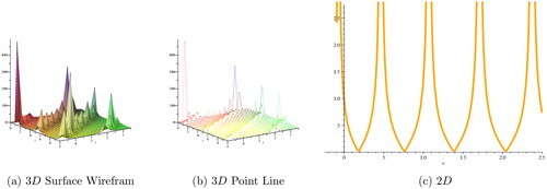
Figure 2. (a, b) 3D and (c) 2D plots, respectively, for ${\Psi }_1(x,t)$ corresponding to the values $\omega =0.5,$ m = 0.3, l = 0.4, z = 2.5, h = 0.3.

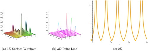
Figure 3. (a, b) 3D and (c) 2D plots, respectively, for ${\Psi }_1(x,t)$ corresponding to the values $\omega =0.5,$ m = 0.3, l = 0.4, z = 2.5, h = 0.3.

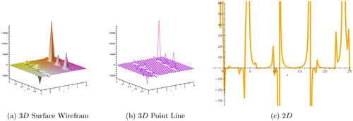
Figure 4. (a, b) 3D and (c) 2D plots, respectively, for ${\Psi }_1(x,t)$ corresponding to the values $\omega =0.5,$ m = 0.3, l = 0.4, z = 2.5, h = 0.3.

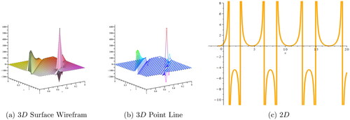
Figure 5. (a, b) 3D and (c) 2D plots, respectively, for ${\Psi }_1(x,t)$ corresponding to the values $\omega =0.5,$ m = 0.3, l = 0.4, z = 2.5, h = 0.3.

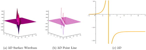
Figure 6. (a, b) 3D and (c) 2D plots, respectively, for ${\Psi }_1(x,t)$ corresponding to the values $\omega =0.5,$ m = 0.3, l = 0.4, z = 2.5, h = 0.3.

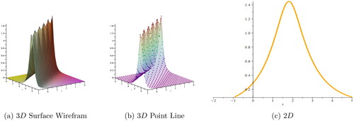
Figure 7. Phase portrait visualization at critical points of the system (28)(28) $$\{\begin{array}{c}\frac{d\Psi }{d\zeta }=\chi ,\hfill \\ \frac{d\chi }{d\zeta }={\eta }_1\Psi -{\eta }_2{\Psi }^2\chi -{\eta }_3{\Psi }^5,\hfill \end{array}$$(28) .

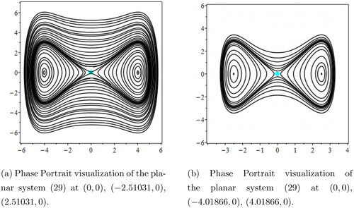
Figure 8. Phase portrait visualization at critical points of the dynamical system (28)(28) $$\{\begin{array}{c}\frac{d\Psi }{d\zeta }=\chi ,\hfill \\ \frac{d\chi }{d\zeta }={\eta }_1\Psi -{\eta }_2{\Psi }^2\chi -{\eta }_3{\Psi }^5,\hfill \end{array}$$(28) .

5. Bifurcation analysis of the model

For the sake of bifurcation analysis through phase portrait of Equation (5)(5) $${\Psi }^{″}+A\Psi +B{\Psi }^2{\Psi }^{\prime }+C{\Psi }^5=0.$$(5) , suppose that ${\Psi }^{\prime }=\chi$ then Equation (5)(5) $${\Psi }^{″}+A\Psi +B{\Psi }^2{\Psi }^{\prime }+C{\Psi }^5=0.$$(5) transforms into the first-order dynamical system of the following form: (28) $$\{\begin{array}{c}\frac{d\Psi }{d\zeta }=\chi ,\hfill \\ \frac{d\chi }{d\zeta }={\eta }_1\Psi -{\eta }_2{\Psi }^2\chi -{\eta }_3{\Psi }^5,\hfill \end{array}$$(28) where ${\eta }_1=\frac{\omega }{l{m}^2},{\eta }_2=\frac{2h}{\mathit{\text{lm}}}$ and ${\eta }_3=\frac{z}{l{m}^2}.$ The dynamical system (28)(28) $$\{\begin{array}{c}\frac{d\Psi }{d\zeta }=\chi ,\hfill \\ \frac{d\chi }{d\zeta }={\eta }_1\Psi -{\eta }_2{\Psi }^2\chi -{\eta }_3{\Psi }^5,\hfill \end{array}$$(28) has the following equilibrium points: $${{\rm Y}}_1=(0,0),\hspace{1em}{{\rm Y}}_2=(-{\left(\frac{{\eta }_1}{{\eta }_3}\right)}^{\frac{1}{4}},0),\hspace{1em}{{\rm Y}}_3=({\left(\frac{{\eta }_1}{{\eta }_3}\right)}^{\frac{1}{4}},0)$$

Furthermore, the Jacobian of (28)(28) $$\{\begin{array}{c}\frac{d\Psi }{d\zeta }=\chi ,\hfill \\ \frac{d\chi }{d\zeta }={\eta }_1\Psi -{\eta }_2{\Psi }^2\chi -{\eta }_3{\Psi }^5,\hfill \end{array}$$(28) is: $$\begin{array}{c}J(\Psi ,\chi )=\left|\begin{array}{cc}0& 1\\ {\eta }_1-2{\eta }_2\Psi \chi -5{\eta }_3{\Psi }^4& 0\end{array}\right|\\ =-{\eta }_1+2{\eta }_2\Psi \chi +5{\eta }_3{\Psi }^4,\end{array}$$ thus $(\Psi ,\chi )$ is a saddle node for $J(\Psi ,\chi )<0,$ a centre when $J(\Psi ,\chi )>0$ and a cusp in case of $J(\Psi ,\chi )=0.$ To investigate the characteristics of the system (28)(28) $$\{\begin{array}{c}\frac{d\Psi }{d\zeta }=\chi ,\hfill \\ \frac{d\chi }{d\zeta }={\eta }_1\Psi -{\eta }_2{\Psi }^2\chi -{\eta }_3{\Psi }^5,\hfill \end{array}$$(28) , we consider the different possible cases by taking various values of parameters and observing the corresponding critical points, the following possible cases are considered and analysed as:

• Case 1: Let ${\eta }_1>0$ ans ${\eta }_2>0.$

For $\omega =0.5,$ m = 0.3, l = 0.4, z = 2.5 and h = 0.3, system (28)(28) $$\{\begin{array}{c}\frac{d\Psi }{d\zeta }=\chi ,\hfill \\ \frac{d\chi }{d\zeta }={\eta }_1\Psi -{\eta }_2{\Psi }^2\chi -{\eta }_3{\Psi }^5,\hfill \end{array}$$(28) , then critical points ${{\rm Y}}_1=(0,0),{{\rm Y}}_2=(-2.510314710,0),$ and ${{\rm Y}}_3=(2.510314710,0).$ In this case, ${{\rm Y}}_1$ is saddle point and ${{\rm Y}}_2,{{\rm Y}}_3$ are central points. The phase plots are displayed for different values of ω in Figure 7.

Figure 9. Sensitivity analysis of the model for initial values $(\Psi ,\chi )=(0.1,0)$ in black (dashed) and $(\Psi ,\chi )=(0.4,0)$ in rainbow (solid).

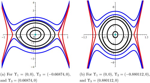
• Case 2: Let ${\eta }_1<0$ ans ${\eta }_2<0.$

For $\omega =-0.5,$ m = 0.3,l = 0.4, $z=-2.5$ and $h=-0.3,$ system (28)(28) $$\{\begin{array}{c}\frac{d\Psi }{d\zeta }=\chi ,\hfill \\ \frac{d\chi }{d\zeta }={\eta }_1\Psi -{\eta }_2{\Psi }^2\chi -{\eta }_3{\Psi }^5,\hfill \end{array}$$(28) exhibits three fixed points ${{\rm Y}}_1=(0,0),{{\rm Y}}_2=(-0.6687403051,0),$ and ${{\rm Y}}_3=(0.6687403051,0).$ In this case, ${{\rm Y}}_1$ is centre and ${{\rm Y}}_2,{{\rm Y}}_3$ are saddle points. Also, the phase plots are displayed for different values of ω in Figure 8.

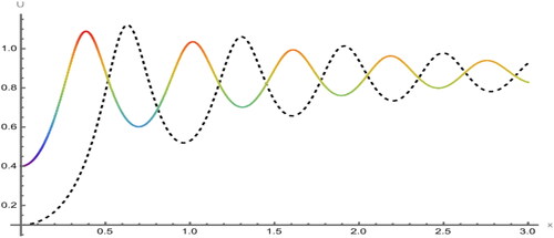
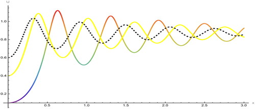
6. Sensitivity analysis

To examine the sensitivity of the proposed model, we have explored three distinct sets of initial conditions. The first set, depicted by the dashed red curve, comprises $(\Psi ,\chi )=(0.1,0);$ the second set, illustrated by the solid blue curve, corresponds to $(\Psi ,\chi )=(0.4,0);$ and the third set, represented by the solid green curve, involves $(\Psi ,\chi )=(0.6,0).$ In Figure 9, two solutions are evident: one for the initial condition $(\Psi ,\chi )=(0.1,0)$ in red and the other for $(\Psi ,\chi )=(0.4,0)$ in blue. Similarly, Figure 10 presents two solutions: $(\Psi ,\chi )=(0.1,0)$ and $(\Psi ,\chi )=(0.6,0).$ Furthermore, Figure 11 displays two solutions: $(\Psi ,\chi )=(0.4,0)$ and $(\Psi ,\chi )=(0.6,0).$ In Figure 12, three solutions are depicted as $(\Psi ,\chi )=(0.1,0),(\Psi ,\chi )=(0.4,0),$ and $(\Psi ,\chi )=(0.6,0).$ It is apparent that slight modifications in the initial conditions can lead to subtle shifts in the outcome of a dynamic system. Consequently, we infer that the proposed system exhibits sensitivity, albeit not to an extreme degree.

Figure 10. Sensitivity analysis of the model for initial values $(\Psi ,\chi )=(0.1,0)$ in red (dashed) and $(\Psi ,\chi )=(0.6,0)$ in blue (solid).

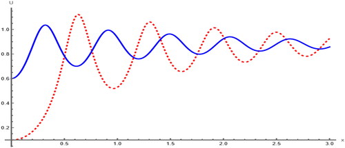
Figure 11. Sensitivity analysis of the model for initial values $(\Psi ,\chi )=(0.1,0)$ in blue (dashed) and $(\Psi ,\chi )=(0.6,0)$ in red (solid).

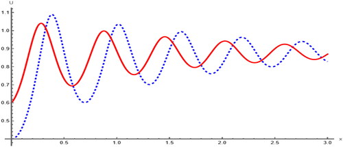
Figure 12. Sensitivity analysis of the model for initial values $(\Psi ,\chi )=(0.1,0)$ in rainbow (solid), $(\Psi ,\chi )=(0.4,0)$ in yellow (solid) and $(\Psi ,\chi )=(0.6,0)$ in black (dashed).

7. Conclusion

In this study, we effectively explored a novel mapping method to the FKE model to unveil novel soliton solutions. This is achieved through the utilization of conformable derivatives by employing the new mapping method and Maple software. Our study elucidates a variety of soliton solutions. These versatile soliton classifications provide flexible tools for both modelling and simulation purposes. To the best of our understanding, new mapping method technique has been employed for the first time on this model, resulting in entirely novel solutions not previously documented in the existing literature. To facilitate comprehension, certain solutions are visually depicted through two-dimensional, three-dimensional plots and phase portraits depicting bifurcation characteristics that explored comprehensively its dynamical nature at equilibrium points utilizing Maple software. Fundamentally, grasping the dynamic characteristics of systems holds significant value in predicting results and propelling advancements in emerging technologies. It is apparent that slight modifications in the initial conditions can lead to subtle shifts in the outcome of a dynamic system. Remarkably, even minor adjustments in initial values lead to considerable variations in the system’s behaviour. In summary, the results of this investigation are not only intriguing but also highlight the effectiveness of the suggested methodologies in evaluating the dynamics of solitons and phase patterns across various nonlinear models.

Author contributions

AUR: investigation and methodology, and writing – original draft, validation. MBR: conceptualization, software, and project administration. OT: formal analysis, visualization, and supervision. All authors have read and agreed to the published version of the manuscript.

Disclosure statement

The authors declare that there is no conflict of interest regarding the publication of this article.

Data availability statement

The data that support the findings of this research are available within this article.

Additional information

Funding

This work was supported by the Ministry of Education, Youth and Sports of the Czech Republic through the e-INFRA CZ (ID: 90254).

References

- Ahmad, M., Zada, A., Ghaderi, M., George, R., & Rezapour, S. (2022). On the existence and stability of a neutral stochastic fractional differential system. Fractal and Fractional, 6(4), 203. doi:10.3390/fractalfract6040203
- Alabedalhadi, M., Al-Omari, S., Al-Smadi, M., & Alhazmi, S. (2023). Traveling wave solutions for time-fractional mKdV-ZK Equation of weakly nonlinear ion-acoustic waves in magnetized electron-positron plasma. Symmetry, 15(2), 361. doi:10.3390/sym15020361
- Alam, M. N., & Tunç, C. (2020a). New solitary wave structures to the (2 + 1)-dimensional KD and KP equations with spatio-temporal dispersion. Journal of King Saud University - Science, 32(8), 3400–3409. doi:10.1016/j.jksus.2020.09.027
- Alam, M. N., & Tunç, C. (2020b). Constructions of the optical solitons and others soliton to the conformable fractional Zakharov-Kuznetsov equation with power law nonlinearity. Journal of Taibah University for Science, 14(1), 94–100. doi:10.1080/16583655.2019.1708542
- Almatrafi, M. B., Ragaa Alharbi, A., & Tunç, C. (2020). Constructions of the soliton solutions to the good Boussinesq equation. Advances in Difference Equations, 2020(1), 14. doi:10.1186/s13662-020-03089-8
- Alam, M. N., Akash, H. S., Saha, U., Hasan, M. S., Parvin, W., & Tunç, C. (2023). Bifurcation analysis and solitary wave analysis of the nonlinear fractional soliton neuron model. Iranian Journal of Science, 47(5–6), 1797–1808. doi:10.1007/s40995-023-01555-y
- Alam, M. N., Iqbal, M., Hassan, M., Al-Asad, M. F., Hossain, M. S., & Tunç, C. (2024). Bifurcation, phase plane analysis and exact soliton solutions in the nonlinear Schrodinger equation with Atangana’s conformable derivative. Chaos, Solitons and Fractals, 182, 114724. doi:10.1016/j.chaos.2024.114724
- Baleanu, D., Aydogn, S. M., Mohammadi, H., & Rezapour, S. (2020). On modelling of epidemic childhood diseases with the Caputo-Fabrizio derivative by using the Laplace Adomian decomposition method. Alexandria Engineering Journal, 59(5), 3029–3039. doi:10.1016/j.aej.2020.05.007
- Baleanu, D., Jajarmi, A., Mohammadi, H., & Rezapour, S. (2020). A new study on the mathematical modelling of human liver with Caputo-Fabrizio fractional derivative. Chaos, Solitons & Fractals, 134, 109705. doi:10.1016/j.chaos.2020.109705
- Batool, A., Talib, I., Riaz, M. B., & Tunç, C. (2022). Extension of lower and upper solutions approach for generalized nonlinear fractional boundary value problems. Arab Journal of Basic and Applied Sciences, 29(1), 249–256. doi:10.1080/25765299.2022.2112646
- Chen, Y., & Wang, Q. (2005). Extended Jacobi elliptic function rational expansion method and abundant families of Jacobi elliptic function solutions to (1 + 1)-dimensional dispersive long wave equation. Chaos, Solitons and Fractals, 24(3), 745–757. doi:10.1016/j.chaos.2004.09.014
- Das, N., & Saha Ray, S. (2022). Dispersive optical soliton wave solutions for the time-fractional perturbed nonlinear Schrödinger equation with truncated M-fractional conformable derivative in the nonlinear optical fibers. Optical and Quantum Electronics, 54, 544.
- Das, N., & Saha Ray, S. (2023). Dispersive optical soliton solutions of the (2 + 1)-dimensional cascaded system governing by coupled nonlinear Schrödinger equation with Kerr law nonlinearity in plasma. Optical and Quantum Electronics, 55, 328.
- Dehingia, K., Mohsen, A. A., Alharbi, S. A., Alsemiry, R. D., & Rezapour, S. (2022). Dynamical behavior of a fractional order model for within-host SARS-CoV-2. Mathematics, 10(13), 2344. doi:10.3390/math10132344
- Filiz, A., Ekici, M., & Sonmezoglu, A. (2014). F-expansion method and new exact solution of the Schrödinger-KdV equation. The Scientific World Journal, 14, 534063.
- Ge, Z.-M., & Ou, C.-Y. (2008). Chaos synchronization of fractional order modified Duffing systems with parameters excited by a chaotic signal. Chaos, Solitons & Fractals, 35(4), 705–717. doi:10.1016/j.chaos.2006.05.101
- Haque, M. A., Zakariya, M. A., Singh, N. S. S., Paul, L. C., & Ishraque, M. F. (2023). Investigation of coupling loss caused by misalignment in optical fiber. Bulletin of Electrical Engineering and Informatics, 12(3), 1560–1569. doi:10.11591/eei.v12i3.4552
- Jiao, M., He, J., He, C., & Alsolami, A. A. (2024). Variational principle for Schrödinger-KdV system with the M-fractional derivatives. Journal of Computational Applied Mechanics, 55(2), 235–241. doi:10.22059/jcamech.2024.374235.1012
- Khalil, R., Al Horani, M., Yousef, A., & Sababheh, M. (2014). A new definition of fractional derivative. Journal of Computational and Applied Mathematics, 264, 65–70. doi:10.1016/j.cam.2014.01.002
- Khan, H., Alam, K., Gulzar, H., Etemad, S., & Rezapour, S. (2022). A case study of fractal-fractional tuberculosis model in China: Existence and stability theories along with numerical simulations. Mathematics and Computers in Simulation, 198, 455–473. doi:10.1016/j.matcom.2022.03.009
- Khater, M. M. A., Ghanbari, B., Nisar, K. S., & Kumar, D. (2020). Novel exact solutions of the fractional Bogoyavlensky-Konopelchenko equation involving the Atangana-Baleanu-Riemann derivative. Alexandria Engineering Journal, 59(5), 2957–2967. doi:10.1016/j.aej.2020.03.032
- Liu, S., Fu, Z., Liu, S., & Zhao, Q. (2001). Jacobi elliptic function expansion method and periodic wave solutions of nonlinear wave equations. Physics Letters A, 289(1–2), 69–74. doi:10.1016/S0375-9601(01)00580-1
- Lü, D. (2005). Jacobi elliptic function solutions for two variant Boussinesq equations. Chaos, Solitons and Fractals, 24(5), 1373–1385. doi:10.1016/j.chaos.2004.09.085
- Mohammed, W. W., El-Morshedy, M., Moumen, A., Ali, E. E., Benaissa, M., & Abouelregal, A. E. (2023). Effects of M-truncated derivative and multiplicative noise on the exact solutions of the breaking soliton equation. Symmetry, 15(2), 288. doi:10.3390/sym15020288
- Naeem, M., Rezazadeh, H., Khammash, A. A., Shah, R., & Zaland, S. (2022). Analysis of the fuzzy fractional-order solitary wave solutions for the KdV equation in the sense of Caputo-Fabrizio derivative. Journal of Mathematics, 2022, 3688916.
- Rabie, W. B., Ahmed, H. M., & Hamdy, W. (2023). Exploration of new optical solitons in magnetooptical waveguide with coupled system of nonlinear Biswas–Milovic equation via Kudryashovís law using extended F-expansion method. Mathematics, 11(2), 300. doi:10.3390/math11020300
- Rafiq, M. N., Majeed, A., Inc, M., & Kamran, M. (2022). New traveling wave solutions for space-time fractional modified equal width equation with beta derivative. Physics Letters A, 446, 128281. doi:10.1016/j.physleta.2022.128281
- Rahmatullah Ellahi, R., Mohyud-Din, S. T., & Khan, U. Exact traveling wave solutions of fractional order Boussinesq-like equations by applying Exp-function method. Results in Physics, 2018, 8, 114–120. doi:10.1016/j.rinp.2017.11.023
- Riaz, M. B., Rehman, A. U., & Martinovic, J. (n.d.). Application of the new mapping method to complex three coupled Maccari’s system possessing M-fractional derivative. Chaos Theory and Applications, 6(3). doi:10.51537/chaos.1414782
- Saha Ray, S., & Das, N. (2022). New optical soliton solutions of fractional perturbed nonlinear Schrödinger equation in nanofibers. Modern Physics Letters B, 36(2), 2150544. doi:10.1142/S0217984921505448
- Senol, M. (2020). New analytical solutions of fractional symmetric regularized-long-wave equation. Revista Mexicana de Física, 66(3 May–Jun), 297–307. doi:10.31349/RevMexFis.66.297
- Tuan, N. H., Mohammadi, H., & Rezapour, S. (2020). A mathematical model for COVID-19 transmission by using the Caputo fractional derivative. Chaos, Solitons, and Fractals, 140, 110107. doi:10.1016/j.chaos.2020.110107
- Vanterler, J., Sousa, D. A. C., Capelas, E., & Oliveira, D. E. (2018). A new truncated M-fractional derivative type unifying some fractional derivative types with classical properties. International Journal of Analysis and Applications, 16, 83–96.
- Vega-Guzman, J., Ullah, M. Z., Asma, M., Zhou, Q., & Biswas, A. (2017). Dispersive solitons in magneto-optic waveguides. Superlattices and Microstructures, 103, 161–170. doi:10.1016/j.spmi.2017.01.020
- Wang, Y.-Y., Su, C.-Q., Liu, X.-Q., & Li, J.-G. (2018). Nonautonomous solitons for an extended forced Korteweg-de Vries equation with variable coefficients in the fluid or plasma. Waves in Random and Complex Media, 28(3), 411–425. doi:10.1080/17455030.2017.1356944
- Zaslavsky, G. M. (2002). Chaos, fractional kinetics, and anomalous transport. Physics Reports, 371(6), 461–580. doi:10.1016/S0370-1573(02)00331-9
- Zayed, E. M.E., & Alurrfi, K. A.E. (2017). Solitons and other solutions for two nonlinear Schrödinger equations using the new mapping method. Optik, 144, 132–148. doi:10.1016/j.ijleo.2017.06.101
- Zeng, X., & Yong, X. (2008). A new mapping method and its applications to nonlinear partial differential equations. Physics Letters A, 372(44), 6602–6607. doi:10.1016/j.physleta.2008.09.025
- Zheng, B., & Feng, Q. (2014). The Jacobi elliptic equation method for solving fractional partial differential equations. Abstract and Applied Analysis, 2014, 9. http://dx.doi.org/10.1155/2014/249071
- Zhu, W., Ling, Z., Xia, Y., & Gao, M. (2023). Bifurcations and the exact solutions of the time-space fractional complex Ginzburg-Landau equation with parabolic law nonlinearity. Fractal and Fractional, 7(2), 201. doi:10.3390/fractalfract7020201