Modelling landscape management scenarios for equitable and sustainable futures in rural areas based on ecosystem services

ABSTRACT

Scenario analysis is a useful technique to inform landscape planning of social-ecological systems by modelling future trends in ecosystem service supply and distribution. This is especially critical in floodplain agroecosystems of rural areas, which are at risk of losing riparian forest corridors due to increasing land use conversion for agricultural production and other ecosystem services due to rural abandonment. However, few studies investigating the effects of land management combine social and ecological modelling in scenario analyses. We estimated the supply of 16 ecosystem services under five alternative scenarios along two gradients: agricultural intensification of the floodplain and active ecological restoration of the riparian forest. We used redundancy analyses to detect ecosystem service bundles and interviews to identify societal gains and losses associated with each management scenario. Our results show how land management influences both the supply and distribution of ecosystem services. Scenarios promoting active ecological restoration supplied more services and benefited a larger range of societal sectors than scenarios focused on provisioning services. We also found two consistent bundles across scenarios, one related to less intensive food supply and another one related to outdoor activities. Interestingly, additional services were included in these bundles in the different scenarios, reflecting land management effects. Landscape scale management promoting both the conservation of ecosystem functioning and the sustainable use of provisioning services could supply a more balanced set of ecosystem services and benefit a larger number of societal sectors, contributing to more equitable and sustainable futures in rural areas.

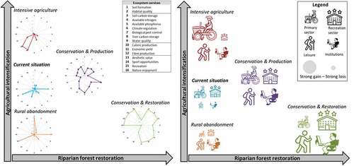
Graphical abstract

EDITED BY:

• Reinette Biggs

KEYWORDS:

• Agricultural system
• multifunctional landscape
• ecosystem management
• land use planning
• floodplain trajectories
• plural valuation

Introduction

Worldwide trends show accelerating rates of urbanization while rural areas undergo depopulation (United Nations 2018). These trends are consistent with shrinking rural regions across Europe, which is particularly strong in Northern and Mediterranean countries (ESPON 2017). For instance, more than 80% of rural municipalities in Spain have shrunk between 1961 and 2011 (ESPON 2017). As a result, a third of provinces in peninsular Spain have currently a population density lower than 30 inhabitants/km², lowering to less than 8 inhabitants/km² in seven provinces (INE 2019). This has resulted in two contrasting landscapes: inhabited rural areas characterized by agricultural intensification and depopulated rural areas characterized by the abandonment of agricultural practices (García-Llorente et al. 2012). It is well known that agricultural intensification can increase the supply of a few provisioning services, such as crop yield, at the expenses of regulating and cultural services (Foley et al. 2005; Felipe-Lucia et al. 2014; Qiu et al. 2021), and it is also associated with biodiversity loss (Allan et al. 2015; Felipe-Lucia and Comín 2015; Newbold et al. 2015). This trade-off is especially critical in floodplain areas, which are threatened by agricultural intensification because of their nutrient-rich soils (Tockner et al. 2008). In turn, natural revegetation following the abandonment of agricultural practices can help improve some ecological functions and services, such as erosion control and water quality (Navarro and Pereira 2015; Darwiche-Criado et al. 2017). However, rural abandonment also has important consequences for the social-ecological system, including the loss of local traditional knowledge associated with low-intensity and semi-subsistence agriculture (Gómez‐Baggethun et al. 2010; Iniesta-Arandia et al. 2014a). In this context, active ecological restoration can enhance multiple ecosystem services and foster the development of rural economies via ecotourism and other nature-based activities (Aradottir and Hagen 2013). Given the varied effects of landscape management on the ecosystem, understanding the social-ecological consequences of the different options is fundamental to inform decision-making on landscape management policies.

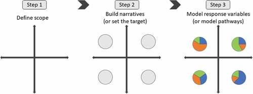
Scenario analysis is a common tool to identify the pros and cons of landscape management according to one or more criteria (Nelson et al. 2009; Kubiszewski et al. 2017; Lerouge et al. 2017). Scenario analysis is generally composed of three steps: definition of scope, design of alternative scenarios (i.e. narratives or storylines) and modelling or assessment of such scenarios (Figure 1). The first step defines the timeframe and extent of the scenario analysis (Kirchgeorg et al. 2010). In the second step, since one of the aims of scenario analyses is to visualize potential end-points and long-term consequences of particular management decisions, the alternatives are designed to show contrasting situations together with intermediate alternatives (Arkema et al. 2015). In the third step, the selection of response variables to be measured against each scenario is critical. In landscape management scenarios, the variables assessed range from biodiversity loss (Liekens et al. 2013) to economic gains (Van Berkel and Verburg 2012). Due to their ability to account for ecological, economic and social values, ecosystem services are gaining importance as key response variables in scenario analyses (Plieninger et al. 2013; Arkema et al. 2015; Rosa et al. 2017).

Figure 1. Main steps for scenario analysis to inform decision-making. Note that steps 2 and 3 are interchangeable depending on the scenario type. Response variables should be inclusive to reflect plural valuation of scenarios (e.g. ecological, social and economic variables), represented by different colours in the pie chart.

Most scenario analyses model a very small set of ecosystem services and neglect the interactive effects of multiple ecosystem services in the landscape in terms of trade-offs and synergies (Bennett et al. 2009; Felipe-Lucia et al. 2014; Qiu et al. 2018). This can lead to important biases in the management decisions informed by those assessments, especially if economic indicators of provisioning services outnumber other indicators and service categories (Martín-López et al. 2014). Therefore, it is important to assess the effect of future scenarios on a variety of ecosystem services, including the often-underrepresented regulating and cultural services, to ensure a better overview of the effects of land management on the ecosystem and to inform policy and decision-making. In this context, the analyses of ecosystem service bundles (i.e. ecosystem services that repeatedly appear together; (Raudsepp-Hearne et al. 2010; Qiu and Turner 2013; Hanspach et al. 2014; Queiroz et al. 2015) can help aggregate the information on multiple ecosystem service indicators and facilitate landscape management by identifying patterns in ecosystem services (Meacham et al. this issue).

Whereas ecosystem services are one type of response variable that can be modelled in scenario analyses, the social component of these scenarios, such as identifying winners and losers, is often neglected or overlooked (Rosa et al. 2017). Indeed, research is increasingly showing that different sectors of society or stakeholders may benefit or lose from alternative land management policies, which can result in strong inequalities between stakeholders (Zafra-Calvo et al. 2017; Benra et al. under review). Despite its critical importance, studies integrating both components of the social-ecological system in scenario analyses by modelling ecological as well as social response variables are few in the literature.

Here, we analyse social and ecological effects of five alternative future scenarios for a Mediterranean agricultural floodplain (Table 1), building on previous knowledge that assessed ecosystem services in different land-use types of the floodplain and social preferences for ecosystem services across a range of stakeholders. The scenarios are based on the combination of two gradients showing typical land management trade-offs: agricultural intensification (i.e. from rural abandonment to intensive agriculture) and ecological restoration (i.e. from the current situation to the active restoration of riparian habitats). Specifically, we i) assess the ecosystem service supply of the five alternative scenarios using proxies of 16 ecosystem services, including supporting, regulating, cultural and provisioning services, ii) identify bundles of ecosystem services that are maintained across scenarios, and iii) investigate the effects of these scenarios on four stakeholder groups in terms of how they are impacted by changes in ecosystem services (i.e. winners and losers). A diagram summarizing the procedures for scenario analysis used in this study can be found in the supplementary Figure S1.

Table 1. Selected ecosystem services, indicators, units, data source and scale of data collection. See supplementary Figure S3 for upscaling and downscaling procedures

Category	Ecosystem service	Indicator	Units	Data source	Scale of data collection
Supporting	Soil formation	Organic matter layer	m^3	Field data	Plot per land use type
	Habitat quality	Riparian Quality Index	-	Field data	Plot per land use type
Regulating	Water quality	Dissolved nitrate	ppm	Field data	Municipality
	Available nitrogen Available phosphorus	Total nitrogen	kg	Field data	Plot per land use type
		Soluble reactive phosphorus	kg	Field data	Plot per land use type
	Soil carbon storage	Total carbon	kg	Field data	Plot per land use type
	Tree carbon storage	Carbon storage in trees	CO2eq	Secondary	Land use type
	Climate regulation	Air temperature variation	°C	Field data	Plot per land use type
	Biological pest control	Vertical vegetation structure	Richness	Field data	Plot per land use type
Provisioning	Food caloric content Food economic yield	Caloric value	kcal	Secondary	Land use type
		Yield	€	Secondary	Land use type
	Fibre production	Biomass increase	T	Secondary	Land use type
Cultural	Aesthetic value	Picture density	Count	Field data	Land use type and municipality
	Recreation	Picnic area density	Count	Field data	Land use type and municipality
	Sport opportunities	Paths density	m	GIS data	Land use type and municipality
	Environmental education	Educational panels	Count	Field data	Land use type and municipality

Materials and methods

Study area

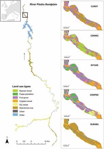
The study area is the floodplain of the River Piedra (River Ebro basin) located in north-east Spain (Figure 2). Annual average temperature is 12.7°C, annual average rainfall is 450 mm, and the water flow is characterized by marked seasonal variability. The River Piedra is approx. 76 km long and the watershed covers an area of 923 km², ranging in altitude from 1100 m.a.s.l. to 600 m.a.s.l. The River Piedra floodplain ranges from 50 to 300 m wide and occupies 19.3 km², covering 12 municipalities with a total area of 532.64 km² and a population of 1539 inhabitants (Felipe-Lucia et al. 2014). The main land use types of the floodplain are dry cereal crops, abandoned croplands, irrigated cereal crops, poplar groves, urban areas, fruit orchards, and riparian forests. The upper part of the River Piedra (ca. 46 km long) is dry for most of the year due to the semiarid climate and karstic substrate, and the main land use type is dry cereal crops. The middle and lower parts of the river have a continuous flow (ca. 30 km long), and the main land use types are irrigated cereal crops, poplar groves, fruit orchards and abandoned croplands. La Tranquera reservoir, built in 1959 with 5.60 km² surface area and 78.8 million m³, is located between the middle and lower lands of the River Piedra, occupying the formerly most productive lands (Felipe-Lucia et al. 2014). Remnants of riparian forests are scattered along the floodplain.

Figure 2. Main land use types of the River Piedra floodplain (left) and example of the effects of alternative management scenarios on the distribution of land use types (right). CURSIT: Current situation; CONRES: Conservation & Restoration; INTAGR: Intensive agriculture; CONPRO: Conservation & Production; RURABA: Rural abandonment (see main text for a full description of the scenarios and Table 2 for a summary).

Table 2. Summary of each scenario. CURSIT: Current situation; CONRES: Conservation & Restoration; INTAGR: Intensive agriculture; CONPRO: Conservation & Production; RURABA: Rural abandonment. NA: Not applicable. PHD: Public Hydraulic Domain (BOE 2008). SCI: Sites of Community Importance designed in the Habitats Directive 92/43/EEC (European Commission 1992). (*) variables considered for the equity assessment but not modelled in the calculations of ecosystem service supply in each scenario

Scenario	Riparian forest	Agriculture	Abandoned cropland	Upper lands	Middle lands	Low lands	Restoration	Tourism*	Water quality	Small dams*
CURSIT	1.6%	43.6%	15.9%	Dry cereal crops	Irrigated cereal crops and poplar groves	Fruit groves, orchards	NA	Centralized and underdeveloped	Same	Kept
CONRES	18.2%	41.1%	2.8%	Dry cereal crops	Irrigated cereal crops and poplar groves	Fruit groves, orchards	5 m PHD + SCI + abandoned croplands> 5000 m^2	Decentralized and developed	+90%	Removed
INTAGR	1.6%	59.4%	0.0%	Dry cereal crops	Irrigated cereal crops, fruit groves and poplar groves	Irrigated cereal crops, fruit groves and poplar groves	NA	Centralized and decrease	−20%	Kept
CONPRO	9.5%	52.6%	0.0%	Dry cereal crops	Dry cereal crops, fruit groves and poplar groves	Dry cereal crops, fruit groves and poplar groves	5 m PHD + SCI	Decentralized and developed	+90%	Removed
RURABA	1.6%	39.2%	20.2%	Dry cereal crops	Irrigated cereal crops and poplar groves	Irrigated cereal crops and poplar groves	NA	Centralized and underdeveloped	+40%	Kept

Identification of social actors

We conducted 71 face-to-face, semi-structured interviews with the main stakeholders of the study area between August 2011 and March 2012 (see locations in supplementary Figure S2). These included the primary sector (i.e. farmers, shepherds, and workers at a fish farm; n = 16), the recreation providers (i.e. owners or workers at restaurants, hotels, lodges, nature tour operators, adventure enterprises, and regional-level tourist site Monasterio de Piedra; n = 13), the recreation users (i.e. retired residents, visitors, hikers, bikers, fishermen; n = 26) and institutions (i.e. local councils, regional governmental bodies for the management of water catchments and natural areas, scientific and educational institutions; n = 16). Interviewees were asked about the uses and benefits they derived from the River Piedra valley. They were also asked to rank a pre-defined list of 21 ecosystem services according to the importance of these services for their livelihoods. Interviews lasted between 30 and 90 minutes and digital records were kept with the interviewees’ consent (see further details in Felipe-Lucia et al. 2015a).

Scenario design

We created five scenarios framed around two typical land management trade-offs (agricultural intensification and active ecological restoration) that could exist in 20 years (Figure 2). These scenarios reflect changes in the ecosystem services ranked highest across all stakeholders and that we were able to measure (e.g. water quality, recreational activities, food production): i) Current situation (CURSIT); ii) Riparian forest conservation and active ecological restoration (CONRES), which strongly influences water quality and recreation; iii) Intensive agriculture (INTAGR), which is related to food production; iv) Riparian forest conservation and agricultural production (CONPRO), which affects most ecosystem services studied; and v) Rural abandonment (RURABA), which represents an existing trend in the study area. The narrative for each scenario is detailed below and summarized in Table 2, indicating the variables included in both the ecological and social assessments or solely in the social assessment.

Current situation (CURSIT)

In the current situation, the River Piedra floodplain is mostly covered by agricultural crops (43.6% of the floodplain), including dry cereal crops in the upper lands, irrigated cereal crops and poplar groves in the middle lands, and fruit groves and orchards in the lower lands. A substantial portion of the study area is abandoned cropland (15.9%). Riparian forest (1.6%) is limited to upland river gorges and to a private natural park located in the middle lands. Tourist activities generated around this park are the main economic driver of the area. There is also a hydropower facility and a fish farm. Pastoralism in the area is rare, with some municipalities having only one or two small-scale shepherds. Companies offering recreational activities in nature start to be developed.

Riparian forest conservation and active ecological restoration (CONRES)

Riparian forest is protected and actively restored across: i) the 5 m of ‘Public Hydraulic Domain’ established by the Spanish law (BOE 2008) along both sides of rivers; ii) Sites of Community Importance (SCI) defined by the European Commission Habitats Directive (92/43/EEC) within the River Piedra floodplain; and iii) abandoned croplands larger than 5000 m² (Osborne and Kovacic 1993; Arizpe et al. 2008). In these areas, typical riparian forest plant species are planted (e.g. Salix sp., Populus sp., Fraxinus sp., etc.) and maintained. Small dams no longer used for irrigation are removed from the stream, facilitating the dispersal of fish and seeds. Restored riparian forests are open to public access, which develops nature tourism based on environmental education, trekking, birdwatching and fishing. Cultivated lands keep the same practices in order to maintain the existing activities of the local population (Barbastro Gil 2005; González et al. 2017).

Intensive agriculture (INTAGR)

Agricultural production is increased by: i) cultivating formerly abandoned croplands; and ii) irrigating all cropland in middle and lower lands. In the upper lands, only water-fed cropland is farmed. In the middle and lower lands, one-third part of the agricultural lands of each municipality are planted with cereals, one-third part with fruit groves and one-third part with poplar groves. Chemical fertilizers and pesticides associated with irrigated cereal crops cause an increase of the pollutant concentrations in the river. As a consequence, negative impacts on the river rise and fishing opportunities are limited to La Tranquera reservoir, decreasing the emerging nature tourism.

Riparian forest conservation and agricultural production (CONPRO)

Riparian forest is protected and actively restored across: i) the 5 m of ‘Public Hydraulic Domain’ established by the Spanish law (BOE 2008) in both riversides; and ii) Sites of Community Importance (SCI) defined by the European Commission Habitats Directive (92/43/EEC) within the River Piedra floodplain. In these areas typical riparian forest species are planted (e.g. Salix sp., Populus sp., Fraxinus sp., etc) and maintained. Agricultural production is increased by farming abandoned cropland. In the upper lands, dry cereal crops are grown. In each municipality of the middle and lower lands, a one-third of abandoned croplands are transformed to dry cereal crops, a one-third to fruit groves and a one-third to poplar groves. Formerly cultivated lands keep same practices in order to maintain the existing activities of the local population (Barbastro Gil 2005; González et al. 2017). Small dams no longer used for irrigation are removed from the stream, facilitating the dispersal of fish and seeds. Restored riparian forests are open to public access, which develops nature tourism based on environmental education, trekking, birdwatching and fishing. Companies offering adventure activities in nature (e.g. climbing, rafting, kayaking) are encouraged. Traditional hydraulic infrastructures (e.g. waterwheels, fulling mill) are restored and ethno-tourism activities increase, fostering the renovation and rental of cottages.

Rural abandonment (RURABA)

Existing investments in agriculture are retained but there are no new investments in irrigation facilities and machinery. This means that the least productive croplands are abandoned. Thus, production is limited to dry cereal crops in the upper lands and irrigated cereal crops and poplar groves in the middle and lower lands. Riparian forests are maintained at their current extent as natural recovery from abandoned cropland in this area takes much longer than 20 years (Moreno-Mateos et al. 2012).

Ecosystem services supply

We estimated 16 indicators of ecosystem services separately for each of the main seven land use types of the study area. The ecosystem services comprised two supporting services, seven regulating services, three provisioning services, and four cultural services (Table 1).

Supporting services

We collected soil data in three plots per land use type except in urban areas, where most of the soils were covered by impervious surfaces. Three transects 25 m apart of each other and perpendicular to the river channel were established in each plot. We collected three samples along each transect at 1 m, 5 m, and 15 m away from the river in July 2011 and July 2012. The organic matter layer depth (cm), excluding leaf litter, was recorded in the field with a measuring tape, and average values at each point across both years were used as an indicator of soil formation. The volume of the soil organic matter layer was calculated in cubic metres. Soils rich in organic matter are more productive (Bauer and Black 1994), and therefore, underly provisioning services.

We estimated habitat quality in three plot replicates per land use type between July 2011 and July 2012 using the Riparian Quality Index (RQI) (González del Tánago and García de Jalón 2011). RQI evaluates seven riverbank attributes: (i) dimensions of land with riparian vegetation (average width of riparian corridor); ii) longitudinal continuity, coverage, and distribution pattern of riparian corridor (woody vegetation); iii) composition and structure of riparian vegetation; iv) age diversity and natural regeneration of woody species; v) bank conditions; vi) floods and lateral connectivity; and vii) substratum and vertical connectivity). RQI results in a relative score between 10 and 120, which was reclassified between 0 and 100. Larger RQI scores indicate better performance of riparian ecological functions (González del Tánago and García de Jalón 2011).

Regulating services

For water quality, we sampled dissolved nitrate as a measure of pollutant concentration in the river (ppm). 21 samples along the river were collected monthly in 2009. The sampling was designed to cover a wide range of situations representing the water quality of the study area and was repeated in specific months of 2010 and 2011 to account for possible variation in the water flow rates. Samples were kept refrigerated and analysed in the laboratory within a week using ionic chromatography (APHA 1998). Values per sample point were averaged across years and then by municipality. As this indicator reflects pollutant concentration, we used the inverse value to account for water quality (Felipe-Lucia et al. 2015b). To model this service in the different scenarios, we considered that the buffer area between the river and the agricultural crops created in the CONRES and CONPRO scenarios can reduce 90% of the water pollution caused by nitrate (Osborne and Kovacic 1993; Parkyn 2004). In turn, it was accounted that the chemical fertilizers and pesticides associated with increasing irrigated cereal crops in the INTAGR scenario cause an increase of 20% in nitrate concentrations in the river (Darwiche-Criado et al. 2017). In the RURABA scenario, the limitation in agricultural production reduces the concentration of nitrate in the water flow by 40% (Darwiche-Criado et al. 2017).

For available nitrogen, we followed the same soil sampling protocol as for soil formation. Nitrogen can be a limiting nutrient for plant growth and condition the functioning of the ecosystem (Vitousek and Howarth 1991; LeBauer and Treseder 2008). Half a kilogram of topsoil (0–10 cm) was collected at each point, dried (48 hours at 60°C), sieved and milled. Total nitrogen (available nitrogen) was measured using a macro elemental analyser (Vario Macro Max CN). Average values across the two sampling campaigns were used as an indicator.

For available phosphorus, we followed the same soil sampling protocol. Phosphorus can be a limiting nutrient for plant growth and condition the functioning of the ecosystem (Vitousek et al. 2010; Lang et al. 2017). Soluble reactive phosphorus (available phosphorus) was extracted following the Olsen protocol (Olsen et al. 1954) and filtered. The extract was analysed in an ionic chromatograph. Average values across the two sampling campaigns were used as an indicator.

For soil carbon storage, we followed the same soil sampling protocol. Soils are an important reservoir of carbon (Lal 2002; Olsson and Ardö 2002). Total carbon was measured using a macro elemental analyser (Vario Macro Max CN). Average values across the two sampling campaigns were used as an indicator.

For tree carbon storage, we used annual CO₂ sequestration rates by land use type from a nationwide study, which estimated the amounts of carbon stored by above- and below-ground biomass of the main Spanish plant species and woody formations (Montero et al. 2005; CITA 2008). Calculations are based on the species annual growth and transformed into CO₂ equivalent tons per hectare using stoichiometric equations (Montero et al. 2005). We used the plant species or woody formations closest to the land cover composition of our study area (e.g. for fruit groves we used average values of apple, pear, peach, and plum groves). Herbaceous species – and therefore, irrigated cereal crops and dry cereal crops – were not included because their annual CO₂ storage balance is null (CITA 2008). For abandoned croplands, only its woody formations (e.g. hawthorn) were considered (Felipe-Lucia et al. 2015b). Urban areas were not included since they usually act as a source of carbon rather than as a sink (but see Davies et al. 2011).

For climate regulation, we recorded air temperature every 60 minutes over a period of 8 months (February to September 2012) using data loggers (iButton). Three devices per plot were hung from trees located at regular distances along a river transect perpendicular to the river channel. Three replicate plots were sampled in representative sites of each selected land use type. Dry cereal crops and fruit groves were not surveyed but surrogate values from abandoned croplands and poplar plantations were used, respectively, due to their similar cover and structure. To estimate local temperature regulation, we used the mean value of the daily temperature range (DTR = maximum temperature of day x – minimum temperature of day x) (Scheitlin and Dixon 2010) per land use type. We took the inverse values (1/DTR) so larger indicator values reflect a larger role in buffering extreme temperatures (Hubbart et al. 2005; Hubbart 2011).

For biological pest control, we estimated the richness of plant strata, as higher plant diversity is expected to host a larger number of insects, thus increasing the probability of biological pest control (Soliveres et al. 2016). We surveyed three plot replicates per land use type in July 2012, except in urban areas. Within each plot, three floodplain-wide transects (average transect length 57 m) perpendicular to the river channel were established 25 m apart. In each transect, we used the point-intercept method (Goodall 1952) every 10 cm to estimate species occurrence and percent cover of each plant species (i.e. number of contacts relative to the total number of points sampled). Identification of plants at the genus or species level was corroborated using a regional herbarium (i.e. herbarium of Jaca: http://proyectos.ipe.csic.es/herbario‎) and a botanist expert. Then, we classified vegetation records into four types of plant strata (i.e. herb, creeper, shrub, and tree) and estimated the richness of plants strata using the vegan package (Oksanen et al. 2013) of the R software (R Core Team 2019).

Provisioning services

For food production, we calculated two indicators, namely, caloric content and economic yield. We estimated the average yield (kilograms per hectare) of each of the main land use types of our study area from the latest update of a national public database (INE 2012), updated on 30.10.2012. For irrigated crops, we averaged the yield values of irrigated wheat, barley, and corn yields. For dry cereal crops, we used averaged yield values of dry wheat, barley, and corn. For fruit groves, we used average yield values of apple, pear, peach, and plum. The rest of land use types were assigned a yield value of 0. To obtain the caloric content per hectare, we multiplied the yield (kilograms per hectare) by the crop caloric content (kilocalories per 100 grams) (Felipe-Lucia et al. 2014). We calculated crop productivity (economic yield) based on crops yield and the index of agricultural prices provided by the regional government (Gobierno de Aragón, http://www.aragon.es) (Felipe-Lucia et al. 2015b).

For fibre production, we used the yearly aboveground dry biomass accumulation by land use type. Data were obtained from a nationwide study that estimated the annual growth rates of woody species as tons of dry biomass per hectare, according to the average timber diameter (Montero et al. 2005; CITA 2008). We adapted data from the closest woody species to the land cover composition of our study area (e.g. for fruit groves we used average data of apple, pear, peach, and plum groves). Herbaceous species – and therefore, irrigated cereal crops and dry cereal crops – were not included because their annual accumulated biomass balance is null (CITA 2008), whereas for abandoned croplands, only its woody formations (e.g. hawthorn) were considered (Felipe-Lucia et al. 2015b). Note that supply of fibre production considers existing management practices, i.e. only supplied by poplar plantations.

Cultural services

For aesthetic value, we used pictures uploaded to Panoramio, a web platform for pictures with a special focus on landscape and environment. This platform has been utilized in previous research about social preferences on ecosystem services (Casalegno et al. 2013; Martínez Pastur et al. 2016; Nahuelhual et al. 2017; Oteros-Rozas et al. 2017). We accessed the platform on 27.03.2014 and counted each single picture taken by a different person in each of the main land use types of the River Piedra floodplain for each municipality. This measure has been considered to be more appropriated than the total number of pictures, which would rather reflect the individual activity of photographers (Casalegno et al. 2013). Pictures focusing on buildings from all sorts (e.g. houses, towers, crosses, churches, hermitages, monasteries, etc.) with no environmental background were excluded because they were not directly related to the use of the ecosystem (Felipe-Lucia et al. 2015b).

For recreation, we counted the number of areas used for social activities (e.g. picnic areas; Posthumus et al. 2010) by land use type and municipality in August 2012. To compare these data across municipalities and land use types, we used a density measure (i.e. Total number of picnic areas by land use type and municipality/Extent of each land use type at each municipality) (Felipe-Lucia and Comín 2015).

For sport opportunities, we downloaded all tracks of sign-posted and user-designed paths from the regional tourist office website (http://senderos.turismodearagon.com) and wikilocs (http://www.wikiloc.com), respectively, available as of 12.10.2012, following Trabucchi et al. (2014). Tracks around the study area were unified using GIS tools (Quantum GIS Development Team 2012), and intersected with the land use cover. Then, we calculated the length of paths per land use and municipality.

For environmental education, we counted the number of educational panels with information about the ecosystem by land use type and municipality in August 2012. To compare these data across municipalities and land use types, we used a density measure (i.e. Total number of educational panels by land use type and municipality/Extent of each land use type at each municipality) (Felipe-Lucia and Comín 2015).

Data analyses

Data on the extension of each land use type per municipality for the CURSIT scenario was extracted from the Spanish crop and land-use digital map (MMAMRM 2009) using ArcGIS 10 (ESRI 2012). The extension for the alternative cenarios was calculated according to the changes in land use described in the narratives above. Note that we did not assume a magnitude of ecosystem services directly from the land use cover maps. Instead, we used our own field sampling or secondary data to map ecosystem services.

Given that we used different scales in the sampling of ecosystem services (e.g. plot per land use type or municipality; Table 1), we upscaled or downscaled ecosystem service measurements to obtain a single value per land use type and/or municipality for each scenario (see supplementary Figure S3). For ecosystem services estimated per unit area of land use type (e.g. food and fibre), we calculated the average supply per hectare for each land use type and multiplied it by the cover of each land use type in each scenario. For ecosystem services estimated at the municipality scale (e.g. cultural services), we divided the supply value by the size of the municipality and multiplied it by the cover of each land use type in that municipality. In the case of water quality, it was not possible to assign a supply value per land use type; therefore, changes in water quality derived from land use changes in each scenario were only estimated at the municipality level, taking as a reference the CURSIT scenario (see Methods for Ecosystem service supply).

In order to facilitate the comparison across scenarios, we normalized ecosystem services to a common scale ranging between 0 and 1 using the formula StV = (x− x_min)/(x_max− x_min); where StV is the normalized variable, x is the target variable and x_min,x_max are the minimum and maximum value across all plots, respectively. We used radial plots to represent the relative supply of ecosystem services under each scenario.

For each scenario, we calculated the relative change in ecosystem service supply from the current situation (i.e. CURSIT scenario) using the formula C = ((t-b)/b)×100; where C is the proportional change in percentage, t is the target value (i.e. the estimated value for the alternative scenarios) and b is the baseline value (i.e. CURSIT scenario).

To identify ecosystem services bundles, we performed a redundancy analysis (RDA), i.e. a multivariate multiple linear regression using the vegan package (Oksanen et al. 2013) in R version 3.6.2 (R Core Team 2019). The supply of each ecosystem service per municipality was the response variable, while the extent in square metres of each of the seven main land use types plus water per municipality was the explanatory variables. Bundles of ecosystem services, i.e. services that repeatedly appear together, sensu Raudsepp-Hearne et al. (2010), in each scenario were identified using both RDA scales 1 and 2, and RDA factor loads (Zoderer et al. 2019). The statistical significance of RDA models and the variance explained by RDA axes were tested by 1000 permutations (Borcard et al. 2011) (supplementary Table S1).

Interviews were transcribed and coded in order to identify the role of each stakeholder group in relation to the studied ecosystem services. We identified stakeholders’ use versus ability to manage each ecosystem service by adapting the existing dependence-influence matrix approach (Reed et al. 2009; Iniesta-Arandia et al. 2014b) and relating this to equity dimensions, as in Felipe-Lucia et al. (2015b) and Martin-Lopez et al. (2019). This information allowed us to identify the stakeholder groups benefiting or losing from each alternative management scenario. We distinguished between strong gain, weak gain, weak loss, and strong loss based on: i) the level of use of ecosystem services of each stakeholder group, which is related to distributive equity; ii) their ability to manage the services they use, which is related to procedural equity; and iii) the increase or decrease in the ecosystem services they use in each scenario. Strong gain was considered when the stakeholder group used and/or managed at least two ecosystem services that improved in that scenario. Strong loss was considered when all or most of the services used by the stakeholder group decreased in that scenario. Weak gains or losses were situations with both improvement and declines in the services used by the stakeholder group, with a slight overall increase (weak gain) or decline (weak loss).

Results

Ecosystem service supply under alternative land management scenarios

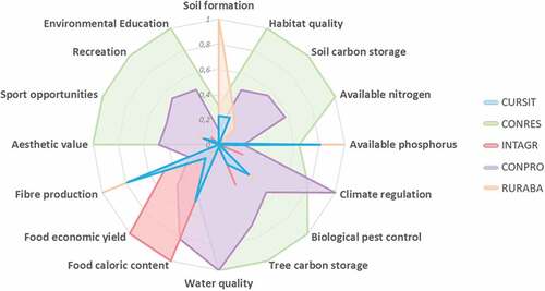
We found large variation in the effects of land management scenarios on ecosystem service supply (Figure 3). Under the Current situation (CURSIT), we observed a low supply of supporting services and most cultural and regulating services but intermediate supply levels for provisioning services in comparison to the other scenarios. Conservation & Restoration (CONRES) achieved the largest supply of cultural services and most supporting and regulating services (excluding soil formation, available phosphorus and climate regulation) but a low supply of provisioning services in relation to other scenarios. This was the scenario with largest ecological gains (Table 3). Intensive agriculture (INTAGR) contributed relatively the least to the supply of supporting services, and most cultural and regulating services (excluding tree carbon storage) and the largest to the supply of food production. This was the scenario with the fewest ecological benefits (Table 3). Conservation & Production (CONPRO) contributed an intermediate supply of most ecosystem services in comparison to the alternative scenarios, maximizing climate regulation and minimizing fibre production. Finally, Rural abandonment (RURABA) contributed relatively the most to soil formation, available phosphorus and fibre production but very little to the remaining ecosystem services.

Table 3. Percentage of change in ecosystem service supply for each scenario in relation to the baseline (i.e. current situation). Positive values (italicized) indicate an increase and negative values (bolded) indicate a loss of ecosystem service supply. No change is denoted in grey font. CONRES: Conservation & Restoration; INTAGR: Intensive agriculture; CONPRO: Conservation & Production; RURABA: Rural abandonment (see text for a full description of the scenarios and Table 2 for a summary)

Ecosystem service	CONRES	INTAGR	CONPRO	RURABA
Soil formation	13.43	−38.46	−18.32	131.10
Habitat quality	39.12	−11.84	12.00	3.61
Water quality	900.00	−16.67	900.00	66.67
Soil carbon storage	6.21	0.01	3.43	1.11
Available nitrogen	13.23	−0.09	7.39	−0.38
Available phosphorus	−6.39	−31.06	−23.59	7.53
Climate regulation	1.21	0.32	1.60	−0.01
Biological pest control	12.86	−6.47	3.85	0.85
Tree carbon storage	255.23	54.16	160.63	−52.25
Food caloric content	−5.27	29.90	11.06	−4.62
Food economic yield	−5.94	66.96	42.26	−63.77
Fibre production	−46.01	−19.78	−31.22	12.48
Aesthetic value	946.43	1.97	448.57	−1.45
Recreation	390.96	18.55	195.90	−15.60
Sport opportunities	198.70	−30.01	72.20	8.49
Environmental education	932.24	0.00	439.99	0.00

Figure 3. Normalized supply of ecosystem services for each scenario (coloured shades). Blue: Current situation (CURSIT); Green: Conservation & Restoration (CONRES); Red: Intensive agriculture (INTAGR); Purple: Conservation & Production (CONPRO); Orange: Rural abandonment (RURABA). Note that the area covered by each scenario is arbitrary (i.e. depends on the sorting of ecosystem services displayed) and should not be used for comparison (see main text for a full description of the scenarios and Table 2 for a summary).

Bundles of ecosystem services across scenarios

The redundancy analysis showed significant relationships between ecosystem services across land management scenarios (supplementary Table S1). In all scenarios, more than 85% of the total variance was explained by the first three axes, with the first axis contributing more than 40% of the total variance, and the second axis adding at least 28% more (supplementary Table S1). In terms of ecosystem services, the first axis separated water quality from the rest of ecosystem services and the second axis separated a group of regulating services from cultural and other services (Figure 4). Regarding land management, the first axis was related to increasing poplar groves and irrigated cereal crops from right to left while the second axis clearly separated dry cereal crops from riparian forests, accompanied by fruit orchards and abandoned croplands in some scenarios.

Figure 4. Redundancy analyses for each scenario. Colours indicate ecosystem service categories (blue: supporting, green: regulating, Orange: provisioning, purple: cultural). Ellipses indicate the bundles (dashed: less intensive food supply bundle, dotted: outdoors activities bundle). CURSIT: Current situation; CONRES: Conservation & Restoration; INTAGR: Intensive agriculture; CONPRO: Conservation & Production; RURABA: Rural abandonment (see main text for a full description of the scenarios and Table 2 for a summary; see supplementary Figure S4 for RDA scaling 2). Note that CURSIT and INTAGR show axis 2 reversed from CONRES, CONPRO and RURABA.

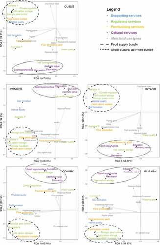
We found two ecosystem services bundles consistent across the five scenarios (Figure 4 and supplementary Figure S4). The first bundle was composed of food caloric content, nitrogen availability, soil carbon storage and biological pest control. In addition, this bundle included additional services in different scenarios, such as climate regulation and habitat quality in CURSIT; climate regulation and fibre production in CONRES; climate regulation, habitat quality and soil formation in INTAGR; and climate regulation in RURABA. In axis 1, the land use types most associated with this first bundle were poplar groves and to a lesser extent irrigated cereal crops; whereas in axis 2, it was positively associated with dry cereal crops and negatively associated with riparian forests (note that in CONRES, this bundle was mostly explained by axis 1 uniquely). The second bundle included all four cultural services and tree carbon storage in all five scenarios; however, it was slightly more scattered in INTAGR, where it also included food economic yield, and in RURABA. In axis 2, this bundle was mostly associated with riparian forest, and to a lesser extent to abandoned crops and fruit orchards, while negatively associated with dry cereal crops. It was only partially explained by axis 1 in CONRES. Surprisingly, food economic yield was not associated with food caloric content in any of the scenarios. In addition, water quality was always unrelated to other services, and partially associated with abandoned croplands and fruit orchards. Other ecosystem services were associated with different bundles in each scenario but did not show a consistent pattern across the five scenarios and, thus, are not further discussed.

Winners and losers of land management scenarios

The land management scenarios had different effects on the total supply of ecosystem services in the study area, with important consequences for the main stakeholders identified (Figure 5). In relation to an optimal situation where all ecosystem services would be supplied in high levels, we observed that under the current situation (CURSIT), both the primary sector and recreation providers have weak losses, because the services that they depend upon are in an average situation. However, the recreation users and institutions have strong loses in CURSIT scenario because the possibilities for individual activities are low and there is little supply of regulating services. Comparing CURSIT with the alternative scenarios, we observe that in CONRES scenario, the primary sector has a weak loss, as some of their cultivated land is turned back to riparian forest. All the other groups have strong gains, as the services they use and manage increase. In INTAGR scenario, the primary sector has strong gains because provisioning services are promoted and the recreation users have weak gains due to the slight increase in cultural ecosystem services. However, the recreation providers have strong losses because water quality deteriorates, and institutions have weak loses because of the decrease in the regulating services that they manage. In CONPRO scenario, all stakeholder groups have weak gains because most services increase in relation to current conditions and there are not major decreases in service supply. In RURABA scenario, both the primary sector and recreation providers have strong losses because of the decrease in both provisioning and cultural services. The recreation users and the institutions have weak losses because some of the regulating services that they use and manage, respectively, slightly increase while others decrease (Table 4).

Table 4. Rationale of the gain and losses of alternative management scenarios on each stakeholder group. CURSIT: Current situation; CONRES: Conservation & Restoration; INTAGR: Intensive agriculture; CONPRO: Conservation & Production; RURABA: Rural abandonment (see text for a full description of the scenarios and Table 2 for a summary)

Stakeholder group	Rationale	CURSIT	CONRES	INTAGR	CONPRO	RURABA
1 Primary sector (e.g. farmers)	Use and have some ability to manage several supporting and regulating services that decrease in INTAGR and improve in CONRES, CONPRO and RURABA, such as biological control, water quality, nutrient regulation (but decreases in RURABA), and soil formation (but decreases in CONPRO). They use and manage food which decreases in CONRES and RURABA and increases in scenarios INTAGR and CONPRO; and fibre, which increases in RURABA and decreases in CONRES, INTAGR and CONPRO. They also use aesthetic and recreation services which increase in all scenarios except RURABA.	Weak loss	Weak loss	Strong gain	Weak gain	Strong loss
2 Recreation providers	Use and manage cultural services which greatly improve in CONRES and CONPRO, have a slight increase in INRAGR and decrease in RURABA. They also use and manage some regulating services such as water quality (which greatly improves in CONRES and CONPRO and decreases in INTAGR) and tree carbon storage (increases in all scenarios but RURABA). They don’t use provisioning services.	Weak loss	Strong gain	Strong loss	Weak gain	Strong loss
3 Recreation users	Use some regulating services (water quality and biological control indirectly) which mostly increase in CONRES and CONPRO but also slightly in RURABA and decrease in INTAGR. They also use cultural services which increase in CONRES (especially high) and CONPRO, slightly in INTAGR and decrease in RURABA. They don’t use provisioning services.	Strong loss	Strong gain	Weak gain	Weak gain	Weak loss
4 Institutions	Manage some of the regulating services that improve in CONRES, CONPRO and RURABA, but decrease in INTAGR, such as water quality and habitat quality. They contribute to tree carbon storage and recreation that increase in CONRES (especially high), INTAGR and CONPRO but decrease in RURABA. They don’t use or manage provisioning services.	Strong loss	Strong gain	Weak loss	Weak gain	Weak loss

Figure 5. Gains and losses of ecosystem services under alternative land management scenarios for the four main stakeholder groups. Coloured icons represent the stakeholder groups in each scenario. Blue: Current situation (CURSIT); Green: Conservation & Restoration (CONRES); Red: Intensive agriculture (INTAGR); Purple: Conservation & Production (CONPRO); Orange: Rural abandonment (RURABA) (see Table 4 for a detailed rationale).

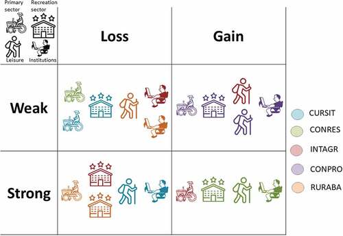
In particular, our results show that while the primary sector (e.g. farmers) would benefit from the most productive scenarios (i.e. INTAGR and CONPRO scenarios), the rest of the stakeholder groups (i.e. recreation providers, recreation users and institutions) would benefit from the scenarios promoting some level of active ecological restoration (i.e. CONRES and CONPRO scenarios). Interestingly, we observed that all stakeholders would lose in RURABA. These results indicate that CONPRO can satisfy the demands of the main stakeholder groups of our study area more equally, while CONRES and INTAGR entail clear winners and losers (i.e. farmers versus the other stakeholder groups) (Figure 5).

Discussion

We analysed the effects of alternative management strategies on ecosystem service supply and stakeholder benefits using scenario analysis. In particular, we identified bundles of ecosystem services that are maintained or changed across scenarios, and explored the social consequences of those scenarios for different stakeholder groups in terms of winners and losers. Our results highlight the importance of combining both ecological and social aspects to inform land planning scenarios that promote multifunctional and inclusive landscapes for different sectors of society (Fischer et al. 2017; Martinez-Sastre et al. 2017).

Understanding patterns in ecosystem services bundles

We found two bundles of ecosystem services consistent across the five scenarios, which highlights the stability of such bundles. The first bundle was related to less intensive food supply, as it combines provisioning (i.e. caloric content) and regulating services. The second bundle was related to outdoors activities around riparian forests. Similar bundles have been identified in other studies (i.e. agroservice and experiential service bundles, respectively; Zoderer et al. 2019). The existence of stable bundles supports the importance of management policies that acknowledge the role of multiple ecosystem services working synergistically rather than focusing on isolated services regardless of their dependencies (Raudsepp-Hearne et al. 2010). In practice, this means that management actions directed to a particular service could also affect other services of the shared bundle, and hence potentially having indirect repercussions on the stakeholders using those related services. In turn, our results also show that additional services can be gained or lost to the bundle depending on the management practices. For example, habitat quality and climate regulation would be lost from the current food supply bundle in Conservation & Production (CONPRO) due to the farming of abandoned croplands. However, in that scenario we could identify a potential third bundle composed of habitat quality, soil formation, phosphorus availability and fibre production.

Our results also show consistent trade-offs in the supply of ecosystem services between management practices preserving the riparian forest versus intensive agriculture. These trade-offs could be reduced by applying soil conservation agriculture measures such as, restoring riparian forest alongside the river, preserving hedgerows, reducing the use of fertilizers and pesticides, and avoiding tilling in fallows (Pretty 2008; Tscharntke et al. 2021). These measures are especially critical in land use types covering larger extents, as these contribute more to the service supply at the landscape scale (Felipe-Lucia et al. 2014). Besides, to promote a more balanced set of ecosystem services, genetic diversity, local knowledge and other cultural services could be enhanced by restoring public paths between farms and along the river, local fruit and fish varieties and fostering active agro-tourism across the valley, as suggested in Conservation & Production (CONPRO). For example, less intensive farming of dry cereal crops could contribute to the conservation and bird-watching of threatened steppe birds such as the Great bustard (Otis tarda) (De Frutos et al. 2015).

Our analyses were based on the most comprehensive dataset available to show the variety of responses of land-use change on a large number of ecosystem services, identifying the potential for synergies and trade-offs among ecosystem service bundles. However, future studies could focus on those services that have been shown to be most important for the different stakeholders and the functioning of the study area, or that are more prone to variation to particular management options. In turn, methods for bundle analysis should be further developed to objectively identify the ecosystem services belonging to the same bundle, regardless of the spread of those services within and across the bundles. For example, the outdoors activities bundle in INTAGR and RURABA was scattered but still a bundle based on RDA scaling 2. Further, a deeper analysis of the stakeholders associated with a bundle could help detecting potential indirect effects, in terms of gains or losses, derived from the management of one or more services within the bundle (Baró et al. 2017; Quintas-Soriano et al. 2019; Zoderer et al. 2019). As in any study, the selection of indicators might compromise the interpretation and extrapolation of our results to other areas where these indicators are not available. Although other studies have reported similar bundles in distinct study sites (Raudsepp-Hearne et al. 2010; Queiroz et al. 2015), the identified bundles could vary if a different set of ecosystem services had been explored. Another potential limitation of our study is due to the fact that the slow recovery times of natural vegetation in Mediterranean areas, especially of riparian vegetation due to increasing droughts, might not reflect the natural recovery following rural abandonment in more humid areas. Therefore, we advise land managers and decision makers to interpret our results with care and to consider the uncertainties associated with the chosen indicators and timescales.

Scenarios for multifunctionality and equity

We found that, despite existing trade-offs, all alternative scenarios analysed increased the supply of ecosystem services, meaning that the Current situation (CURSIT) is under-supplying ecosystem services relative to its potential in the study area. Interestingly, we found that Rural abandonment (RURABA) only enhanced a few services but decreased the majority; emphasizing the importance of a proactive landscape management instead of simply ‘abandoning rural areas to their fate’ if we are to avoid losses of ecosystem services at the landscape scale (Posthumus et al. 2010; Rouquette et al. 2011). This result highlights how current trends in rural abandonment in many European (e.g. Portugal, Germany, Greece, Romania; ESPON 2017), and North American (Li and Li 2017) countries is an immediate threat for ecosystem service supply (Bruno et al. 2021). Scenario modelling can contribute to avoiding further losses by forecasting the consequences of those changes. In order to advise landscape management, it is thus important that scenario analyses incorporate intermediate solutions together with situations of complete change (Arkema et al. 2015), such as landscape intensification, rural abandonment and active ecological restoration. Additional considerations should include the availability of funding and land to implement those actions (Comín et al. 2018).

Our study also illustrates how identifying the most suitable alternative management scenario depends not only on the preferred ecosystem services to be enhanced, but also on the interest of decision-makers in distributing service benefits equally across stakeholder groups. For instance, in our case study, the Intensive agriculture (INTAGR) scenario would be most adequate to increase provisioning services, but it would only strongly benefit the primary sector. On the other hand, the Conservation & Restoration (CONRES) scenario would maximize most ecosystem services and benefit most stakeholder groups, but at the expense of losses to the primary sector due to a reduction in provisioning services. The latter scenario would make it difficult to maintain the local population, given that most inhabitants of the study area are farmers (Felipe-Lucia et al. 2015a). Therefore, in order to supply and distribute a more balanced set of ecosystem services, an intermediate land use management strategy would be more appropriate, as was also found in other areas in Spain (García-Llorente et al. 2012; Martinez-Sastre et al. 2017). In our case study, this could be achieved in the Conservation & Production (CONPRO) scenario, which promotes provisioning services while preserving and enhancing cultural, regulating and supporting services. Such combination is key to nurturing a more equal distribution of ecosystem services across the main stakeholder groups. Therefore, decision-making should not only be informed by which scenarios contribute more to overall ecosystem services (multifunctionality), but also by who are the beneficiaries of these services (Martinez-Sastre et al. 2017). Incorporating the analyses of power asymmetries among stakeholders is, thus, critical to balance the dominance of particular interests over common goals (Berbés-Blázquez et al. 2016).

Multifunctionality research and metrics are rapidly evolving in sustainability sciences, from considering multiple ecosystem functions, to services and stakeholders at the landscape scale (Manning et al. 2018; Hölting et al. 2019), but it still needs to go one step further to incorporate issues of equity in the distribution of ecosystem services. Previous research has shown that different aspects of equity (i.e. procedural, distributive and recognition) are important to ensure access to ecosystem services (Vallet et al. 2019; Zafra-Calvo et al. 2019), and that the relations between stakeholders at multiple spatial scales shape access to ecosystem services (Martin-Lopez et al. 2019). Our results support decision-making that takes into account the needs of different stakeholders by clearly indicating the winners and losers of alternative management scenarios. In this way, decision-makers are informed of both the ecological and social consequences of policies and are provided with alternatives to balance inequalities derived from land management strategies. In particular, our scenario Conservation & Production (CONPRO) contributes weak gains to all four main stakeholder groups without placing any of them in a vulnerable situation as losers of the decision-making process. Therefore, this scenario could be used as a strategy to promote equity in the access to ecosystem services among the main stakeholder groups of the studied area. On the contrary, our results show that other scenarios would favour some stakeholder groups while disfavouring other groups, hence, causing inequalities in the access to ecosystem services. Scenario analysis is an excellent tool to identify long-term effects of landscape planning, but needs to incorporate stakeholder analyses to understand the different facets of landscape management if we are to design scenarios promoting truly sustainable landscapes, i.e. inclusive to different sectors of society and that offer equal opportunities of access and benefits to all of them. Our approach can, thus, guide further research aiming at plural valuation (Jacobs et al. 2020) for sustainability by combining the assessment of multifunctionality and equity associated with alternative management scenarios.

Management policies for rural areas

High-level agricultural policies, such as the Common Agricultural Policy (CAP) in Europe, should be able to support multifunctional landscapes. However, despite the promotion of new greening measures, the CAP is not having the expected positive benefits (Pe’er et al. 2019) and seems to still be driving both agricultural intensification and rural depopulation in many European countries (Martinez-Sastre et al. 2017). In our case study, multifunctional landscapes would be achieved through the scenario Conservation and Production (CONPRO), but its implementation would only be feasible if the suggested reforms of the current CAP are followed, such as, supporting public goods, biodiversity conservation and active restoration, together with participatory and integrative landscape scale planning (Pe’er et al. 2020). In addition, future research should continue to investigate the limits of ecosystems’ ability to supply services within a socially just space (Raworth 2017), if we are to advice environmental management policies and design realistic scenarios for rural areas.

Because of the multiplicity of policies applicable in rural areas, it can be complicated to simultaneously comply with all of them at the local scale (Baur 2020). Adaptive management systems to particular ecological and societal conditions, integrated within multi-layered governance systems, should be promoted to ensure coherence in the implementation of policies at different spatial scales (Nagendra and Ostrom 2012; Hölting et al. 2019; Winkler et al. 2021). The development of flexible institutions open to public participation are essential to develop learning and adaptation needed in the face of new situations. For example, in our scenario Conservation & Production (CONPRO), poly-centric governance could cope with conflicts derived from new management practices in rural areas, such as the combination of traditional agricultural practices with increasing agro-tourism (Castro et al. 2011; Nagendra and Ostrom 2012).

Conclusion

Scenario planning based on ecosystem services is a useful tool to forecast the effects of alternative landscape management on ecological and social variables. Studies need to consider a varied range of ecosystem services, at least in the initial phase, in order to be comprehensive, identify synergies and trade-offs, and detect the existence of ecosystem service bundles, as we do here. We found evidence of two consistent bundles of ecosystem services across different scenarios (related to less intensive food supply and outdoor activities), and identified the ecosystem services that are lost or added to the bundle depending on the scenario’s management regime. Our results highlight the importance of considering ecosystem services in land management to avoid the loss of potential services and to include stakeholder analyses to identify winner and losers of the alternative management options. The combination of both types of information (i.e. social and ecological) is crucial to achieve truly sustainable landscapes, which maximize the number of services (multifunctional) and stakeholder groups benefiting from them (equal). In our case study, and probably in many other similar contexts, an intermediate management scenario preserving both the conservation of natural resources and the local productive uses of the ecosystem might be the best compromise in the long-term. Our approach can be used as a method to assess the sustainability of future scenarios in rural areas, based on the analyses of procedural and distributive equity of ecosystem services, taking into account the synergies and trade-offs derived from the alternative management scenarios.

Disclosure statement

No potential conflict of interest was reported by the author(s).

Supplementary material

Supplemental data for this article can be accessed here

References

- Allan E, Manning P, Alt F, Binkenstein J, Blaser S, Blüthgen N, Böhm S, Grassein F, Hölzel N, Klaus VH, et al. 2015. Land use intensification alters ecosystem multifunctionality via loss of biodiversity and changes to functional composition. Ecol Lett. 18:834–843. doi:10.1111/ele.12469.
- APHA. 1998. Standard methods for the examination of water and wastewater. 20th ed. Washington (DC): American Public Health Association.
- Aradottir AL, Hagen D. 2013. Chapter three - ecological restoration: approaches and impacts on vegetation, soils and society. In: Sparks DL, editor. Advances in agronomy. Academic Press;p. 173–222. doi:10.1016/B978-0-12-407686-0.00003-8.
- Arizpe D, Mendes A, Rabaça JE. 2008. Sustainable riparian zones. A management guide. Valencia (Spain): Ripidurable-Generalitat Valenciana.
- Arkema KK, Verutes GM, Wood SA, Clarke-Samuels C, Rosado S, Canto M, Rosenthal A, Ruckelshaus M, Guannel G, Toft J, et al. 2015. Embedding ecosystem services in coastal planning leads to better outcomes for people and nature. Proc Natl Acad Sci. 112:7390–7395. doi:10.1073/pnas.1406483112.
- Barbastro Gil L. 2005. El Monasterio de Piedra: historia y paisaje turístico Zaragoza (Spain): Ibercaja, Obra Social y Cultural.
- Baró F, Gómez-Baggethun E, Haase D. 2017. Ecosystem service bundles along the urban-rural gradient: insights for landscape planning and management. Ecosyst Serv. 24:147–159. doi:10.1016/j.ecoser.2017.02.021.
- Bauer A, Black AL. 1994. Quantification of the effect of soil organic matter content on soil productivity. Soil Sci Soc Am J. 58:185–193. doi:10.2136/sssaj1994.03615995005800010027x.
- Baur P. 2020. When farmers are pulled in too many directions: comparing institutional drivers of food safety and environmental sustainability in California agriculture. Agric Hum Values. 37:1175–1194. doi:10.1007/s10460-020-10123-8.
- Bennett EM, Peterson GD, Gordon LJ. 2009. Understanding relationships among multiple ecosystem services. Ecol Lett. 12:1394–1404. doi:10.1111/j.1461-0248.2009.01387.x.
- Benra F, Nahuelhual L, Felipe-Lucia M, Bonn A. under review. Context matters - designing equitable and balanced PES strategies. Ecosyst Serv.
- Berbés-Blázquez M, González JA, Pascual U. 2016. Towards an ecosystem services approach that addresses social power relations. Curr Opin Environ Sustain Sustainability Sci. 19:134–143. doi:10.1016/j.cosust.2016.02.003.
- BOE. 2008. Dominio Público Hidráulico [WWW Document]. Minist Pres Esp BOE–2008-755. [accessed 2020 April 24]. https://www.boe.es/boe/dias/2008/01/16/pdfs/A03141-03149.pdf.
- Borcard D, Gillet F, Legendre P. 2011. Canonical ordination. In: Borcard D, Gillet F, Legendre P, editors. Numerical ecology with R, Use R. New York (NY): Springer; p. 153–225. doi:10.1007/978-1-4419-7976-6_6.
- Bruno D, Sorando R, Álvarez-Farizo B, Castellano C, Céspedes V, Gallardo B, Jiménez JJ, López MV, López-Flores R, Moret-Fernández D, et al. 2021. Depopulation impacts on ecosystem services in Mediterranean rural areas. Ecosyst Serv. 52:101369. doi:10.1016/j.ecoser.2021.101369.
- Casalegno S, Inger R, DeSilvey C, Gaston KJ. 2013. Spatial Covariance between Aesthetic Value & Other Ecosystem Services. PLoS ONE. 8:e68437. doi:10.1371/journal.pone.0068437.
- Castro AJ, Martin-Lopez B, Garcia-llorente M, Aguilera PA, Lopez E, Cabello J. 2011. Social preferences regarding the delivery of ecosystem services in a semiarid Mediterranean region. J Arid Environ. 75:1201–1208. doi:10.1016/j.jaridenv.2011.05.013.
- CITA. 2008. Estudio sobre la funcionalidad de la vegetación leñosa de aragon como sumidero de CO2: existencias y potencialidad (estimación cuantitativa y predicciones de fijación) Informe final Diciembre. Zaragoza (Spain): Centro de Investigación y Tecnología Agroalimentaria de Aragón.
- Comín FA, Miranda B, Sorando R, Felipe‐Lucia MR, Jiménez JJ, Navarro E. 2018. Prioritizing sites for ecological restoration based on ecosystem services. J Appl Ecol. 55:1155–1163. doi:10.1111/1365-2664.13061.
- Council Directive 92/43/EEC of 21 May. 1992. On the conservation of natural habitats and of wild fauna and flora. http://data.europa.eu/eli/dir/1992/43/oj/eng
- Darwiche-Criado N, Comín FA, Masip A, García M, Eismann SG, Sorando R. 2017. Effects of wetland restoration on nitrate removal in an irrigated agricultural area: the role of in-stream and off-stream wetlands. Ecol Eng. 103:426–435. doi:10.1016/j.ecoleng.2016.03.016.
- Davies ZG, Edmondson JL, Heinemeyer A, Leake JR, Gaston KJ. 2011. Mapping an urban ecosystem service: quantifying above-ground carbon storage at a city-wide scale. J Appl Ecol. 48:1125–1134. doi:10.1111/j.1365-2664.2011.02021.x.
- De Frutos A, Olea PP, Mateo-Tomás P. 2015. Responses of medium- and large-sized bird diversity to irrigation in dry cereal agroecosystems across spatial scales. Agric Ecosyst Environ. 207:141–152. doi:10.1016/j.agee.2015.04.009.
- ESPON. 2017. Policy brief on shrinking rural regions in Europe.
- ESRI. 2012. ArcGIS Desktop. Redlands (CA): Environmental Systems Research Institute.
- Felipe-Lucia MR, Comín FA. 2015. Ecosystem services–biodiversity relationships depend on land use type in floodplain agroecosystems. Land Use Policy. 46:201–210. doi:10.1016/j.landusepol.2015.02.003.
- Felipe-Lucia MR, Comín FA, Bennett EM. 2014. Interactions among ecosystem services across land uses in a floodplain agroecosystem. Ecol Soc. 19. doi:10.5751/ES-06249-190120.
- Felipe-Lucia MR, Comín FA, Escalera-Reyes J. 2015a. A framework for the social valuation of ecosystem services. AMBIO. 44:308–318. doi:10.1007/s13280-014-0555-2.
- Felipe-Lucia MR, Martín-López B, Lavorel S, Berraquero-Díaz L, Escalera-Reyes J, Comín FA. 2015b. Ecosystem services flows: why stakeholders’ power relationships matter. PLoS ONE. 10:e0132232. doi:10.1371/journal.pone.0132232.
- Fischer J, Meacham M, Queiroz C. 2017. A plea for multifunctional landscapes. Front Ecol Environ. 15:59. doi:10.1002/fee.1464.
- Foley JA, DeFries R, Asner GP, Barford C, Bonan G, Carpenter SR, Chapin FS, Coe MT, Daily GC, Gibbs HK, et al. 2005. Global consequences of land use. Science. 309:570–574. doi:10.1126/science.1111772.
- García-Llorente M, Martín-López B, Iniesta-Arandia I, López-Santiago CA, Aguilera PA, Montes C. 2012. The role of multi-functionality in social preferences toward semi-arid rural landscapes: an ecosystem service approach. Environ Sci Policy. 19–20:136–146. doi:10.1016/j.envsci.2012.01.006.
- Gómez‐Baggethun E, Mingorría S, Reyes‐García V, Calvet L, Montes C. 2010. Traditional ecological knowledge trends in the transition to a market economy: empirical study in the doñana natural areas. Conserv Biol. 24:721–729. doi:10.1111/j.1523-1739.2009.01401.x.
- González del Tánago M, García de Jalón D. 2011. Riparian Quality Index (RQI): a methodology for characterising and assessing the environmental conditions of riparian zones. Limnetica. 30:235–254.
- González E, Felipe-Lucia MR, Bourgeois B, Boz B, Nilsson C, Palmer G, Sher AA. 2017. Integrative conservation of riparian zones. Biol Conserv. 211:20–29. doi:10.1016/j.biocon.2016.10.035.
- Goodall DW. 1952. Quantitative aspects of plant distribution. Biol Rev. 27:194–242. doi:10.1111/j.1469-185X.1952.tb01393.x.
- Hanspach J, Hartel T, Milcu AI, Mikulcak F, Dorresteijn I, Loos J, Von Wehrden H, Kuemmerle T, Abson D, Kovács-Hostyánszki A, et al. 2014. A holistic approach to studying social-ecological systems and its application to southern Transylvania. Ecol Soc. 19. doi:10.5751/ES-06915-190432.
- Hölting L, Jacobs S, Felipe-Lucia MR, Maes J, Norström AV, Plieninger T, Cord AF. 2019. Measuring ecosystem multifunctionality across scales. Environ Res Lett. 14:124083. doi:10.1088/1748-9326/ab5ccb.
- Hubbart JA. 2011. An inexpensive alternative solar radiation shield for ambient air temperature and relative humidity micro-sensors. J Nat Environ Sci. 2:9–14.
- Hubbart J, Link T, Campbell C, Cobos D. 2005. Evaluation of a low‐cost temperature measurement system for environmental applications. Hydrol Process. 19:1517–1523. doi:10.1002/hyp.5861.
- INE. 2012. Anuario Estadístico Agrario. Madrid (Spain): Instituto Nacional de Estadística.
- INE. 2019. Península Ibérica en cifras. Instituto Nacional de Estadística. [accessed 2020 April 22]. https://ine.es/prodyser/pubweb/pin/pin2019/18/index.html.
- Iniesta-Arandia I, Del Amo DG, García-Nieto AP, Piñeiro C, Montes C, Martín-López B. 2014a. Factors influencing local ecological knowledge maintenance in Mediterranean watersheds: insights for environmental policies. AMBIO. 1–12. doi:10.1007/s13280-014-0556-1.
- Iniesta-Arandia I, García-Llorente M, Aguilera PA, Montes C, Martín-López B. 2014b. Socio-cultural valuation of ecosystem services: uncovering the links between values, drivers of change, and human well-being. Ecol Econ. 108:36–48. doi:10.1016/j.ecolecon.2014.09.028.
- Jacobs S, Zafra-Calvo N, Gonzalez-Jimenez D, Guibrunet L, Benessaiah K, Berghöfer A, Chaves-Chaparro J, Díaz S, Gomez-Baggethun E, Lele S, et al. 2020. Use your power for good: plural valuation of nature – the Oaxaca statement. Glob Sustain. 3. doi:10.1017/sus.2020.2.
- Kirchgeorg M, Jung K, Klante O. 2010. The future of trade shows: insights from a scenario analysis. J Bus Ind Mark. 25:301–312. doi:10.1108/08858621011038261.
- Kubiszewski I, Costanza R, Anderson S, Sutton P. 2017. The future value of ecosystem services: global scenarios and national implications. Ecosyst Serv. 26:289–301. doi:10.1016/j.ecoser.2017.05.004.
- Lal R. 2002. Soil carbon dynamics in cropland and rangeland. Environ Pollut. 116:353–362.
- Lang F, Krüger J, Amelung W, Willbold S, Frossard E, Bünemann EK, Bauhus J, Nitschke R, Kandeler E, Marhan S, et al. 2017. Soil phosphorus supply controls P nutrition strategies of beech forest ecosystems in Central Europe. Biogeochemistry. 136:5–29. doi:10.1007/s10533-017-0375-0.
- LeBauer DS, Treseder KK. 2008. Nitrogen limitation of net primary productivity in terrestrial ecosystems is globally distributed. Ecology. 89:371–379. doi:10.1890/06-2057.1.
- Lerouge F, Gulinck H, Vranken L. 2017. Valuing ecosystem services to explore scenarios for adaptive spatial planning. Ecol Indic. 81:30–40. doi:10.1016/j.ecolind.2017.05.018.
- Li S, Li X. 2017. Global understanding of farmland abandonment: a review and prospects. J Geogr Sci. 27:1123–1150. doi:10.1007/s11442-017-1426-0.
- Liekens I, Schaafsma M, De Nocker L, Broekx S, Staes J, Aertsens J, Brouwer R. 2013. Developing a value function for nature development and land use policy in Flanders, Belgium. Land Use Policy. 30:549–559. doi:10.1016/j.landusepol.2012.04.008.
- Manning P, Plas F, Soliveres S, Allan E, Maestre FT, Mace G, Whittingham MJ, Fischer M. 2018. Redefining ecosystem multifunctionality. Nat Ecol Evol. 2:427–436. doi:10.1038/s41559-017-0461-7.
- Martin-Lopez B, Felipe-Lucia MR, Bennett EM, Norstrom A, Peterson G, Plieninger T, Hicks CC, Turkelboom F, Garcia-Llorente M, Jacobs S, et al. 2019. A novel telecoupling framework to assess social relations across spatial scales for ecosystem services research. J Environ Manage. 241:251–263. doi:10.1016/j.jenvman.2019.04.029.
- Martín-López B, Gómez-Baggethun E, García-Llorente M, Montes C. 2014. Trade-offs across value-domains in ecosystem services assessment. Ecol Indic Part A. 37:220–228. doi:10.1016/j.ecolind.2013.03.003.
- Martínez Pastur G, Peri PL, Lencinas MV, García-Llorente M, Martín-López B. 2016. Spatial patterns of cultural ecosystem services provision in Southern Patagonia. Landsc Ecol. 31:383–399. doi:10.1007/s10980-015-0254-9.
- Martinez-Sastre R, Ravera F, Gonzalez JA, Lopez Santiago C, Bidegain I, Munda G. 2017. Mediterranean landscapes under change: combining social multicriteria evaluation and the ecosystem services framework for land use planning. LAND USE POLICY. 67:472–486. doi:10.1016/j.landusepol.2017.06.001.
- MMAMRM. 2009. Mapa de cultivos y aprovechamientos, actualización 2000–2009. Escala 1:50000. Madrid (Spain): Ministerio de Medio Ambiente Y Medio Rural y Marino.
- Montero G, Ruiz-Peinado R, Muñoz M. 2005. Producción de biomasa y fijación de CO2 por los bosques españoles. Madrid: Instituto Nacional de Investigación y Técnica Agraria y Alimentaria.
- Moreno-Mateos D, Power ME, Comín FA, Yockteng R. 2012. Structural and functional loss in restored wetland ecosystems. PLoS Biol. 10:e1001247. doi:10.1371/journal.pbio.1001247.
- Nagendra H, Ostrom E. 2012. Polycentric governance of multifunctional forested landscapes. Int J Commons. 6(2):104. doi:10.18352/ijc.321.
- Nahuelhual L, Vergara X, Kusch A, Campos G, Droguett D. 2017. Mapping ecosystem services for marine spatial planning: recreation opportunities in Sub-Antarctic Chile. Mar Policy. 81:211–218. doi:10.1016/j.marpol.2017.03.038.
- Navarro LM, Pereira HM. 2015. Rewilding abandoned landscapes in Europe. In: Pereira HM, and Navarro LM, editors. Rewilding European landscapes. Springer International Publishing; p. 3–23 doi:10.1007/978-3-319-12039-3.
- Nelson E, Mendoza G, Regetz J, Polasky S, Tallis H, Cameron D, Chan KM, Daily GC, Goldstein J, Kareiva PM, et al. 2009. Modeling multiple ecosystem services, biodiversity conservation, commodity production, and tradeoffs at landscape scales. Front Ecol Environ. 7:4–11. doi:10.1890/080023.
- Newbold T, Hudson LN, Hill SLL, Contu S, Lysenko I, Senior RA, Börger L, Bennett DJ, Choimes A, Collen B, et al. 2015. Global effects of land use on local terrestrial biodiversity. Nature. 520:45–50. doi:10.1038/nature14324.
- Oksanen J, Blanche G, Friendly M, Kindt R, Legendre P, McGlinn D. 2013. Vegan: community ecology package. R Package Version. 2 0.10 [WWW Document]. [accessed 2020 April 24]. https://cran.r-project.org/web/packages/vegan/vegan.pdf.
- Olsen SR, Cole CV, Watanabe FS, Dean LA. 1954. Estimation of available phosphorus in soils by extraction with sodium bicarbonate. USDA Circular. Washington (DC): Government Printing Office.
- Olsson L, Ardö J. 2002. Soil carbon sequestration in degraded semiarid agro-ecosystems—perils and potentials. Ambio. 31:471–477. doi:10.1639/0044-7447(2002)031[0471:SCSIDS2.0.CO;2.
- Osborne LL, Kovacic DA. 1993. Riparian vegetated buffer strips in water-quality restoration and stream management. Freshw Biol. 29:243–258. doi:10.1111/j.1365-2427.1993.tb00761.x.
- Oteros-Rozas E, Martín-López B, Fagerholm N, Bieling C, Plieninger T. 2017. Using social media photos to explore the relation between cultural ecosystem services and landscape features across five European sites. Ecol Indic. 94. doi:10.1016/j.ecolind.2017.02.009.
- Parkyn S. 2004. Review of riparian buffer zone effectiveness. Wellington (UK): Ministry of Agriculture and Forestry.
- Pe’er G, Bonn A, Bruelheide H, Dieker P, Eisenhauer N, Feindt PH, Hagedorn G, Hansjürgens B, Herzon I, Lomba Â, et al. 2020. Action needed for the EU Common Agricultural Policy to address sustainability challenges. People Nat. 2:305–316. doi:10.1002/pan3.10080.
- Pe’er G, Zinngrebe Y, Moreira F, Sirami C, Schindler S, Müller R, Bontzorlos V, Clough D, Bezák P, Bonn A, et al. 2019. A greener path for the EU Common Agricultural Policy. Science. 365:449–451. doi:10.1126/science.aax3146.
- Plieninger T, Bieling C, Ohnesorge B, Schaich H, Schleyer C, Wolff F. 2013. Exploring futures of ecosystem services in cultural landscapes through participatory scenario development in the Swabian Alb, Germany. Ecol Soc. 18. doi:10.5751/ES-05802-180339.
- Posthumus H, Rouquette JR, Morris J, Gowing DJG, Hess TM. 2010. A framework for the assessment of ecosystem goods and services; a case study on lowland floodplains in England. Ecol Econ. 69:1510–1523. doi:10.1016/j.ecolecon.2010.02.011.
- Pretty J. 2008. Agricultural sustainability: concepts, principles and evidence. Philos Trans R Soc Lond B Biol Sci. 363:447–465. doi:10.1098/rstb.2007.2163.
- Qiu J, Carpenter SR, Booth EG, Motew M, Zipper SC, Kucharik CJ, Loheide SP II, Turner MG. 2018. Understanding relationships among ecosystem services across spatial scales and over time. Environ Res Lett. 13:054020. doi:10.1088/1748-9326/aabb87.
- Qiu J, Queiroz C, Bennett EM, Cord AF, Crouzat E, Lavorel S, Maes J, Meacham M, Norström AV, Peterson GD, et al. 2021. Land-use intensity mediates ecosystem service tradeoffs across regional social-ecological systems. Ecosyst People. 17:264–278. doi:10.1080/26395916.2021.1925743.
- Qiu J, Turner MG. 2013. Spatial interactions among ecosystem services in an urbanizing agricultural watershed. Proc Natl Acad Sci. 201310539. doi:10.1073/pnas.1310539110.
- Quantum GIS Development Team. 2012. Quantum GIS Desktop (1.8.0). Beaverton (Oregon): Open Source Geospatial Foundation Project.
- Queiroz C, Meacham M, Richter K, Norström AV, Andersson E, Norberg J, Peterson G. 2015. Mapping bundles of ecosystem services reveals distinct types of multifunctionality within a Swedish landscape. AMBIO. 44:89–101. doi:10.1007/s13280-014-0601-0.
- Quintas-Soriano C, García-Llorente M, Norström A, Meacham M, Peterson G, Castro AJ. 2019. Integrating supply and demand in ecosystem service bundles characterization across Mediterranean transformed landscapes. Landsc Ecol. 34:1619–1633. doi:10.1007/s10980-019-00826-7.
- R Core Team. 2019. R: a language and environment for statistical computing. [WWW Document]. Vienna Austria: R Foundation for Statistical Computing. [accessed 2020 April 24]. https://www.eea.europa.eu/data-and-maps/indicators/oxygen-consuming-substances-in-rivers/r-development-core-team-2006.
- Raudsepp-Hearne C, Peterson GD, Bennett EM. 2010. Ecosystem service bundles for analyzing tradeoffs in diverse landscapes. Proc Natl Acad Sci. doi:10.1073/pnas.0907284107.
- Raworth K. 2017. A Doughnut for the Anthropocene: humanity’s compass in the 21st century. Lancet Planet Health. 1:e48–e49. doi:10.1016/S2542-5196(17)30028-1.
- Reed MS, Graves A, Dandy N, Posthumus H, Hubacek K, Morris J, Prell C, Quinn CH, Stringer LC. 2009. Who’s in and why? A typology of stakeholder analysis methods for natural resource management. J Environ Manage. 90:1933–1949. doi:10.1016/j.jenvman.2009.01.001.
- Rosa IMD, Pereira HM, Ferrier S, Alkemade R, Acosta LA, Akcakaya HR, Den Belder E, Fazel AM, Fujimori S, Harfoot M, et al. 2017. Multiscale scenarios for nature futures. Nat Ecol Evol. 1:1416–1419. doi:10.1038/s41559-017-0273-9.
- Rouquette JR, Posthumus H, Morris J, Hess TM, Dawson QL, Gowing DJG. 2011. Synergies and trade-offs in the management of lowland rural floodplains: an ecosystem services approach. Hydrol Sci J -J Sci Hydrol. 56:1566–1581. doi:10.1080/02626667.2011.629785.
- Scheitlin KN, Dixon PG. 2010. Diurnal temperature range variability due to land cover and airmass types in the southeast. J Appl Meteorol Climatol. 49:879–888. doi:10.1175/2009JAMC2322.1.
- Soliveres S, van der Plas F, Manning P, Prati D, Gossner MM, Renner SC, Alt F, Arndt H, Baumgartner V, Binkenstein J, et al. 2016. Biodiversity at multiple trophic levels is needed for ecosystem multifunctionality. Nature. 536:456–459. doi:10.1038/nature19092.
- Tockner K, Bunn SE, Gordon C, Naiman RJ, Quinn GP, Stanford JA. 2008. Flood plains: critically threatened ecosystems. In: Polunin NVC, editor. Aquatic ecosystems. Cambridge: Cambridge University Press; p. 45–62. doi:10.1017/CBO9780511751790.006.
- Trabucchi M, O’Farrell PJ, Notivol E, Comín FA. 2014. Mapping ecological processes and ecosystem services for prioritizing restoration efforts in a semi-arid mediterranean River Basin. Environ Manage. 1–14. doi:10.1007/s00267-014-0264-4.
- Tscharntke T, Grass I, Wanger TC, Westphal C, Batáry P. 2021. Beyond organic farming – harnessing biodiversity-friendly landscapes. Trends Ecol Evol. 36:919–930. doi:10.1016/j.tree.2021.06.010.
- United Nations. 2018. The World’s Cities in 2018 - Data Booklet, Statistical Papers - United Nations (Ser. A), Population and Vital Statistics Report. United Nations Department of Economic and Social Affairs, Population Division. doi:10.18356/8519891f-en.
- Vallet A, Locatelli B, Levrel H, Dendoncker N, Barnaud C, Quispe Conde Y. 2019. Linking equity, power, and stakeholders’ roles in relation to ecosystem services. Ecol Soc. 24. doi:10.5751/ES-10904-240214.
- Van Berkel DB, Verburg PH. 2012. Combining exploratory scenarios and participatory backcasting: using an agent-based model in participatory policy design for a multi-functional landscape. Landsc Ecol. 27:641–658. doi:10.1007/s10980-012-9730-7.
- Vitousek PM, Howarth R. 1991. Nitrogen limitation on land and in the sea: how can it occur? Biogeochemistry. 13:87–115. doi:10.1007/BF00002772.
- Vitousek PM, Porder S, Houlton BZ, Chadwick OA. 2010. Terrestrial phosphorus limitation: mechanisms, implications, and nitrogen–phosphorus interactions. Ecol Appl. 20:5–15. doi:10.1890/08-0127.1.
- Winkler KJ, Rodrigues JG, Albrecht E, Crockett ETH. 2021. Governance of ecosystem services: a review of empirical literature. Ecosyst People. 17:306–319. doi:10.1080/26395916.2021.1938235.
- Zafra-Calvo N, Garmendia E, Pascual U, Palomo I, Gross-Camp N, Brockington D, Cortes-Vazquez J-A, Coolsaet B, Burgess ND. 2019. Progress toward equitably managed protected areas in Aichi Target 11: a global survey. BioScience. 69:191–197. doi:10.1093/biosci/biy143.
- Zafra-Calvo N, Pascual U, Brockington D, Coolsaet B, Cortes-Vazquez JA, Gross-Camp N, Palomo I, Burgess ND. 2017. Towards an indicator system to assess equitable management in protected areas. Biol Conserv. 211:134–141. doi:10.1016/j.biocon.2017.05.014.
- Zoderer BM, Tasser E, Carver S, Tappeiner U. 2019. Stakeholder perspectives on ecosystem service supply and ecosystem service demand bundles. Ecosyst Serv. 37:100938. doi:10.1016/j.ecoser.2019.100938.