Identifying critical transitions in major depression with fuzzy recurrence entropy

ABSTRACT

Detection of mood changes can be useful for the efficacy of drug treatment of psychiatric disorders in major depression. This paper presents an approach for detecting major time points of mood transitions under the influence of antidepressants. These time points, which are indicated by critical fluctuations in time series, can be discovered using change point detection and time-frequency analysis of fuzzy recurrence entropy of mood data. The mood transitions identified by the fuzzy recurrence entropy agree with results that were clinically validated and reported in literature. The proposed approach can detect early mood transitions in a fully objective way that does not require the manual analysis of fluctuations in the signal dynamics.

KEYWORDS:

• Fuzzy recurrence entropy
• nonlinear dynamics
• major depression
• critical transitions

Introduction

Major depression or depressive disorder is also known as clinical depression, which describes a serious mood disorder that is a type of mental illness caused by life events or grieving. Effects of major depression are severe as they adversely affect the emotion, thinking, and daily activities of the patient. Signs and symptoms of depression are highly variable among individuals. Some may experience only a few symptoms while others may experience many. The severity and frequency of depressive symptoms as well as their duration highly depend on the specific illness of individuals.

Evidence of early warning signals (EWSs) in depression has recently been reported by utilizing the theory of complex system dynamics, which opens a new door to discovering the onset and termination of depression (van de Leemput et al. 2014), understanding and evaluation of personalized risk in the transitions of continuous episodes of major depression in individuals (Wichers and Groot 2016), and detecting sudden changes toward lower symptom severity and sudden changes toward higher symptom severity in mood disorders (Olthof et al. 2020). The interest in the use of critical slowing down and critical fluctuations as an EWS for identifying critical transitions in complex systems has been growing (Wen et al. 2018). The concept of EWSs is introduced as indicators for regime shifts in complex systems (Scheffer et al. 2009, 2012). In other words, an EWS is a period that shows critical fluctuations or critical slowing down in the signals of the complex system under study. Such a period refers to an unstable state that occurs after and before stable states of the system. An EWS can be used to predict an imminent transition between stable states in patients receiving psychotherapy for mood disorders, and therefore there is a reason to expect that it may be useful in patients being treated with antidepressants (Olthof et al. 2020).

Recurrence is a natural phenomenon recorded in time series of human mental states. Therefore, methods for studying recurrence dynamics are potential for discovering complex patterns in depression data (Wichers and Groot 2016). A publicly available data of major depression obtained during a double-blind experiment of reduction in antidepressant dosage is studied herein. The previous study (Pham 2020b) applied the method of fuzzy recurrence plots and tensor decomposition for visualizing the results of different stages of the dose-reduction experiment using only a few moods.

Although the data adopted in this study consist of a single subject clinically diagnosed with major depression, the measurement design of the data is very useful for identifying EWSs within single individuals (Wichers and Groot 2016). The detection of sudden shifts in mental states has the potential to provide precise information about personalized risks of transitions in depression (Bos and De Jonge 2014; Wichers and Groot 2016). These sudden shifts may anticipate an implication of either undesirable or desirable changes (Scheffer et al. 2012). There has been no study or data being able to provide observations of direct evidence to cover a proven critical change in mood and adequate number of observations prior to that change to allow for the measure of EWSs. ‘This case experiment presents precisely such data. It was conducted by a mental health care user (hereafter: the participant) who collected 1474 prospective momentary observations of daily life experiences’ (Wichers and Groot 2016).

The motivation for the work proposed in this study was two-fold. First, it contributes to the demand for developing a technically sound approach for early detection of mood changes in major depression. Second, while existing methods lack fully objective analysis of critical fluctuations in time series, the proposed approach provides not only a rigorous algorithm for objective analysis but also the reproducibility of results with fully automated processes. The contributions of the research reported in this paper are highlighted as follows. The use of the Shannon entropy and fuzzy entropy of fuzzy recurrence plots (Pham 2020a) is useful for detecting EWSs in major depression under the reduction of medication. The study enables the integration of multiple moods of mental health and provides a novel way for the analysis of very short time series of the moods expressed in integers obtained from answers to questionnaire. The proposed approach is yet simple and general for practical computer implementations in complex time-series analysis in psychometrics that aims to provide quantitative measures in psychology and social sciences.

Materials and methods

Data

The time series were obtained from a male participant at the age of 57 years, who was diagnosed with major depressive disorder and had been using antidepressants for 8.5 years at the time of the experiment (Wichers and Groot 2016). Records of 19 mood states were obtained from the participant for up to 10 times a day over a period of 239 days. His temporary states of mind were measured with a momentary assessment questionnaire using a 7-point Likert scale, ranging either from 1 (not) to 7 (very) or from -3 (not) to 3 (very).

The participant initiated the experiment because the participant wished to know if he might be exposed to the possibility of being at risk of developing any new episode of depression during the period of gradual reduction of the antidepressants, and if the vulnerability could be detected in the data. The pharmacist, who was selected by the participant, provided a dose-reduction scheme that was randomly chosen out of several dose-reduction schemes. In this experiment, both the participant and involved researchers were not given information about the dose-reduction scheme; however, they were aware that reduction in antidepressant dosage was to be applied by the pharmacist.

The experimental procedures consisted of 5 phases (Kossakowski et al. 2017). Phase 1 is a baseline measurement period that lasted for four weeks. Phase 2 is a double-blind period in which there was no reduction in the antidepressant dosage, which lasted for two weeks. Phase 3 is a double-blind period in which gradual reduction in the antidepressant dosage (venlafaxine) was made from 150 mg to 0 mg, which lasted for eight weeks. Phase 4 is a post-assessment period in which the antidepressant dosage was not changed (the venlafaxine dosage was kept at 0), which lasted for eight weeks. Phase 5 is a follow-up period that lasted for twelve weeks. Descriptions of the 19 moods are shown in Table 1. Figures 1–6 show the time series of the 19 moods recorded for the entire time and broken down by each phase, respectively.

Figure 1. Time series of 19 moods in all 5 phases. (a) mood 1; (b) mood 2; (c) mood 3; (d) mood 4; (e) mood 5; (f) mood 6; (g) mood 7; (h) mood 8; (i) mood 9; (j) mood 10; (k) mood 11; (l) mood 12; (m) mood 13; (n) mood 14; (o) mood 15; (p) mood 16; (q) mood 17; (r) mood 18; (s) mood 19.

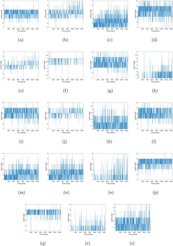
Figure 2. Time series of 19 moods in Phase 1. (a) mood 1; (b) mood 2; (c) mood 3; (d) mood 4; (e) mood 5; (f) mood 6; (g) mood 7; (h) mood 8; (i) mood 9; (j) mood 10; (k) mood 11; (l) mood 12; (m) mood 13; (n) mood 14; (o) mood 15; (p) mood 16; (q) mood 17; (r) mood 18; (s) mood 19.

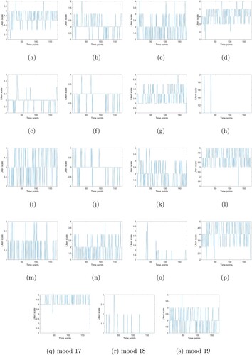
Figure 3. Time series of 19 moods in Phase 2. (a) mood 1; (b) mood 2; (c) mood 3; (d) mood 4; (e) mood 5; (f) mood 6; (g) mood 7; (h) mood 8; (i) mood 9; (j) mood 10; (k) mood 11; (l) mood 12; (m) mood 13; (n) mood 14; (o) mood 15; (p) mood 16; (q) mood 17; (r) mood 18; (s) mood 19.

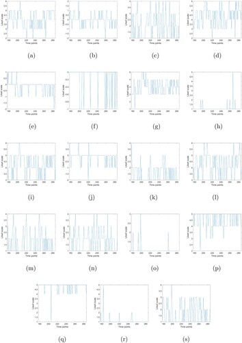
Figure 4. Time series of 19 moods in Phase 3. (a) mood 1; (b) mood 2; (c) mood 3; (d) mood 4; (e) mood 5; (f) mood 6; (g) mood 7; (h) mood 8; (i) mood 9; (j) mood 10; (k) mood 11; (l) mood 12; (m) mood 13; (n) mood 14; (o) mood 15; (p) mood 16; (q) mood 17; (r) mood 18; (s) mood 19.

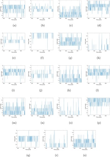
Figure 5. Time series of 19 moods in Phase 4. (a) mood 1; (b) mood 2; (c) mood 3; (d) mood 4; (e) mood 5; (f) mood 6; (g) mood 7; (h) mood 8; (i) mood 9; (j) mood 10; (k) mood 11; (l) mood 12; (m) mood 13; (n) mood 14; (o) mood 15; (p) mood 16; (q) mood 17; (r) mood 18; (s) mood 19.

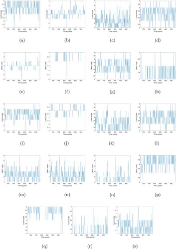
Figure 6. Time series of 19 moods in Phase 5. (a) mood 1; (b) mood 2; (c) mood 3; (d) mood 4; (e) mood 5; (f) mood 6; (g) mood 7; (h) mood 8; (i) mood 9; (j) mood 10; (k) mood 11; (l) mood 12; (m) mood 13; (n) mood 14; (o) mood 15; (p) mood 16; (q) mood 17; (r) mood 18; (s) mood 19.

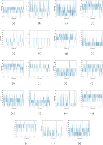
Table 1. Nineteen momentary mood states (Kossakowski et al. 2017).

Mood number	Mood states	7-point Likert scale
1	I feel relaxed	1 (not) to 7 (very)
2	I feel down	−3 (not) to 3 (very)
3	I feel irritated	1 (not) to 7 (very)
4	I feel satisfied	1 (not) to 7 (very)
5	I feel lonely	−3 (not) to 3 (very)
6	I feel anxious	−3 (not) to 3 (very)
7	I feel enthusiastic	1 (not) to 7 (very)
8	I feel suspicious	1 (not) to 7 (very)
9	I feel cheerful	1 (not) to 7 (very)
10	I feel guilty	−3 (not) to 3 (very)
11	I feel indecisive	1 (not) to 7 (very)
12	I feel strong	1 (not) to 7 (very)
13	I feel restless	1 (not) to 7 (very)
14	I feel agitated	1 (not) to 7 (very)
15	I worry	1 (not) to 7 (very)
16	I can concentrate well	1 (not) to 7 (very)
17	I like myself	1 (not) to 7 (very)
18	I am ashamed of myself	1 (not) to 7 (very)
19	I doubt myself	1 (not) to 7 (very)

Regarding ethical issues: ‘The participant (the 2nd author of the data paper Kossakowski et al. 2017) initiated the study and expressed that he wanted the data to be published. Approval from the Maastricht University ethical committee was therefore unnecessary and not obtained. The participant gave his consent for collecting and (re)using the data.’ Kossakowski et al. (2017).

0.2. Fuzzy recurrence entropy

Recurrence is an important concept for studying the dynamics of nonlinear time series. Mathematical methods for quantifying recurrence have been developed in chaos theory and nonlinear data analysis. A popular approach for the analysis of recurrence is the method of recurrence plots (Eckmann et al. 1987) and its extended algorithms. A recurrence plot (RP) provides a visualization of the revisits of time points of a phase-space set reconstructed from the original time series. Such revisits are called recurrences that give insight into complex behaviors of a dynamical system.

In mathematical terms, the formulation of an RP can be described as follows (Marwan et al. 2007). Let $\mathbf{X}=\{{\mathbf{x}}_1,{\mathbf{x}}_2,\dots ,{\mathbf{x}}_N\}\in {\mathbb{R}}^{Nm}$, where ${\mathbf{x}}_i=(x_{i1},\dots ,x_{im})$, $i=1,2,\dots ,N$, be a set of state vectors of the phase-space reconstruction of a dynamical system, in which ${\mathbf{x}}_i\in {\mathbb{R}}^m$ is the state of the dynamical system at time i in an embedding dimension m. A recurrence plot (RP) is expressed an $N\times N$ matrix, in which an element of an RP, denoted as $\mathbf{R}(i,j)$, is represented with a black dot if the distance between ${\mathbf{x}}_i$ and ${\mathbf{x}}_j$ is considered to be closed to each other. In other words, if ${\mathbf{x}}_i$ and ${\mathbf{x}}_j$ are similar, then there is an indication of recurrence. Two states ${\mathbf{x}}_j$ and ${\mathbf{x}}_i$ are said to be close or similar to each other if the distance between the two states is within the radius ${\mathbf{r}}_i$ whose center is ${\mathbf{x}}_i$. Because ${\mathbf{r}}_i$ and ${\mathbf{r}}_j$ may not be the same, this measure of similarity between two states of the phase-space reconstruction of a dynamical system can result in an asymmetrical RP.

To make an RP symmetrical, a threshold, denoted as ϵ, is used to define the closeness or similarity of a state pair $({\mathbf{x}}_i,{\mathbf{x}}_j)$ as follows (Marwan et al. 2007): (1) $\mathbf{R}(i,j)=\theta (ϵ-\Vert {\mathbf{x}}_i-{\mathbf{x}}_j\Vert ),$(1) where $\theta (\cdot )$ is the step function defined as (2) $\theta (ϵ-\Vert {\mathbf{x}}_i-{\mathbf{x}}_j\Vert )=\{\begin{array}{ll}1& :ϵ-\Vert {\mathbf{x}}_i-{\mathbf{x}}_j\Vert \ge 0\\ 0& :ϵ-\Vert {\mathbf{x}}_i-{\mathbf{x}}_j\Vert <0\end{array}$(2) A black dot is assigned to an element $(i,j)$ of an RP if $\mathbf{R}(i,j)$ = 1, otherwise an RP element $(i,j)$ is represented with a white dot if $\mathbf{R}(i,j)$ = 0. Thus, an RP can be visualized as a binary square image.

A recurrence plot mostly contains dots and lines. The main diagonal of the plot is called the line of identity (LOI). Diagonal lines are those that are parallel or orthogonal to the LOI. The length of a diagonal line is the number of connected dots that form the line. The Shannon entropy of an RP is defined as (3) $H_{\mathrm{R}\mathrm{P}}=-\sum _{l=l_{min}}^{N}p\left(l\right)\ln \left(p\right(l\left)\right),$(3) where (4) $p\left(l\right)=\frac{P\left(l\right)}{\sum _{l=l_{min}}^{N}P\left(l\right)}.$(4) in which $l_{min}$ is the minimum length of the diagonal lines of an RP, and $P\left(l\right)$ is the frequency distribution of length l of the diagonal lines of the RP.

A fuzzy recurrence plot (FRP) (Pham 2016) attempts to overcome the problem of defining a good similarity threshold imposed for constructing an RP. The mathematical formulation of an FRP is based on the concept of the theory of fuzzy sets for the inference of similarity (Zadeh 1971). A fuzzy set (Zadeh 1965) is defined as a set whose elements have grades of fuzzy membership, taking values of real numbers. Mathematically, let U be a universe of discourse and A a subset of U. A fuzzy set A is characterized by a fuzzy membership function ${\mu }_A\left(x\right)$ that maps each element $x\in U$ to the interval [0, 1]. Thus, ${\mu }_A\left(x\right)$ is called the fuzzy membership grade of x in A. The greater value of ${\mu }_A\left(x\right)$ is, the more possible x is an element of A.

The mathematical formulation of an FRP is described as follows (Pham 2016). Once again, let $\mathbf{X}=({\mathbf{x}}_1,\dots ,{\mathbf{x}}_N)$ be a collection of the state vectors of the reconstructed phase space of a time series. Given $\mathbf{X}$, a pre-defined number of clusters c, and using the fuzzy c-means (FCM) algorithm (Bezdek 1981), a set of fuzzy clusters $\mathbf{V}=\{{\mathbf{v}}_1,\dots ,{\mathbf{v}}_c\}$ and the fuzzy membership grades expressing the degrees of the state vectors ${\mathbf{x}}_i\in \mathbf{X}$ belonging to cluster centers ${\mathbf{v}}_k\in \mathbf{V}$ can be determined to represent the partition of $\mathbf{X}$.

A fuzzy recurrence plot, denoted by $\tilde{\mathbf{R}}$, is defined as (5) $\tilde{\mathbf{R}}(i,j)=\mu ({\mathbf{x}}_i,{\mathbf{x}}_j),i,j=1,\dots ,N,$(5) where $\mu ({\mathbf{x}}_i,{\mathbf{x}}_j)\in [0,1]$ is the fuzzy membership of similarity between ${\mathbf{x}}_i$ and ${\mathbf{x}}_j$, which can be inferred using the three properties of fuzzy relations as follows.

1. Reflexivity: (6) $\mu ({\mathbf{x}}_i,{\mathbf{x}}_i)=1,i=1,\dots ,N.$(6)

2. Symmetry: (7) $\begin{array}{rl}\mu ({\mathbf{x}}_i,{\mathbf{v}}_k)& =\mu ({\mathbf{v}}_k,{\mathbf{x}}_i),\\ & i=1,\dots ,N,k=1,\dots ,c.\end{array}$(7)

3. Transitivity: (8) $\begin{array}{rl}\mu ({\mathbf{x}}_i,{\mathbf{x}}_j)& =max[min\{\mu ({\mathbf{x}}_i,{\mathbf{v}}_k),\mu ({\mathbf{x}}_j,{\mathbf{v}}_k)\left\}\right],\\ & k=1,\dots ,c;i\ne j.\end{array}$(8)

The purpose of the fuzzy c-means (FCM) is to minimize the following objective function: (9) $F_w(\mathbf{U},\mathbf{V})=\sum _{k=1}^N\sum _{i=1}^c({\mu }_{ik}{)}^w\Vert {\mathbf{x}}_k-{\mathbf{v}}_i{\Vert }^2,$(9) where

$\mathbf{X}=({\mathbf{x}}_1,\dots ,{\mathbf{x}}_N)\in {\mathbb{R}}^{Nm}$ = the data,

c = the number of clusters in $\mathbf{X}$, $2\le c<N$,

${\mu }_{ik}$ = fuzzy membership grade of ${\mathbf{x}}_k$ in cluster ${\mathbf{v}}_i$, ${\mu }_{ik}\in [0,1]$,

w = fuzzy weighting exponent, $1\le w<\mathrm{\infty }$

$\mathbf{U}$ = $c\times N$ fuzzy c-partition of $\mathbf{X}$, where the elements of $\mathbf{U}$ are the fuzzy membership grades of N data points in c clusters,

$\mathbf{V}=({\mathbf{v}}_1,\dots ,{\mathbf{v}}_c\}$ = clusters of $\mathbf{X}$,

${\mathbf{v}}_i=(v_{i1},\dots ,v_{in})$ = center of cluster i,

$\Vert \cdot \Vert$ = is the Euclidean norm.

The squared distance between ${\mathbf{x}}_k$ and ${\mathbf{v}}_i$ expressed in Equation (9(9) $F_w(\mathbf{U},\mathbf{V})=\sum _{k=1}^N\sum _{i=1}^c({\mu }_{ik}{)}^w\Vert {\mathbf{x}}_k-{\mathbf{v}}_i{\Vert }^2,$(9) ) is computed in the A-norm as (10) $d_{ik}^2=\Vert {\mathbf{x}}_k-{\mathbf{v}}_i{\Vert }^2=({\mathbf{x}}_k-{\mathbf{v}}_i{)}^T({\mathbf{x}}_k-{\mathbf{v}}_i).$(10) The above objective function is subject to (11) $\sum _{i=1}^c{\mu }_{ik}=1,k=1,\dots ,N.$(11) The most popular norms for use with the objective function defined in Equation (9(9) $F_w(\mathbf{U},\mathbf{V})=\sum _{k=1}^N\sum _{i=1}^c({\mu }_{ik}{)}^w\Vert {\mathbf{x}}_k-{\mathbf{v}}_i{\Vert }^2,$(9) ) is the Euclidean norm, which is applied in this study for constructing FRPs. The minimization of the objective function of the FCM is numerically carried out by an iterative process of updating the fuzzy membership grades and cluster centers until the convergence or maximum number of iterations is reached. The fuzzy membership grades and cluster centers are iteratively updated as (12) $\begin{array}{rl}{\mu }_{ik}& =\frac{1}{\sum _{q=1}^c{\left(\frac{\Vert {\mathbf{x}}_k-{\mathbf{v}}_i\Vert }{\Vert {\mathbf{x}}_k-{\mathbf{v}}_q\Vert }\right)}^{2/(w-1)}};\end{array}$(12) (13) $\begin{array}{rl}{\mathbf{v}}_i& =\frac{\sum _{k=1}^N({\mu }_{ik}{)}^w{\mathbf{x}}_k}{\sum _{k=1}^N({\mu }_{ik}{)}^w},i=1,\dots ,c.\end{array}$(13) The iterative procedure of the FCM is outlined as follows.

1. Given c, w, step t, $t=0,\dots ,T$, initialize matrix ${\mathbf{U}}^{(t=0)}=[{\mu }_{ik}{]}^{(t=0)}$

2. Compute ${\mathbf{v}}_i^{\left(t\right)}$, $i=1,\dots ,c$, using Equation (13(13) $\begin{array}{rl}{\mathbf{v}}_i& =\frac{\sum _{k=1}^N({\mu }_{ik}{)}^w{\mathbf{x}}_k}{\sum _{k=1}^N({\mu }_{ik}{)}^w},i=1,\dots ,c.\end{array}$(13) ).

3. Update ${\mathbf{U}}^{(t+1)}$ using Equation (12(12) $\begin{array}{rl}{\mu }_{ik}& =\frac{1}{\sum _{q=1}^c{\left(\frac{\Vert {\mathbf{x}}_k-{\mathbf{v}}_i\Vert }{\Vert {\mathbf{x}}_k-{\mathbf{v}}_q\Vert }\right)}^{2/(w-1)}};\end{array}$(12) ).

4. If $\Vert {\mathbf{U}}^{(t+1)}-|{\mathbf{U}}^{\left(t\right)}\Vert <ϵ$ or t = T, stop. Otherwise, set ${\mathbf{U}}^{\left(t\right)}={\mathbf{U}}^{(t+1)}$ and return to step 2.

Having presented the formulation of an FRP, the Shannon entropy of an FRP, denoted as $H_{\mathrm{F}\mathrm{R}\mathrm{P}}$, can be defined as (14) $H_{\mathrm{F}\mathrm{R}\mathrm{P}}=-\sum _{i=}^N\sum _{j=1}^N\mu ({\mathbf{x}}_i,{\mathbf{x}}_j){\log }_2\left[\mu \right({\mathbf{x}}_i,{\mathbf{x}}_j\left)\right].$(14) Following the definition of the Shannon entropy of an FRP, the fuzzy entropy of an FRP, denoted as $F_{\mathrm{F}\mathrm{R}\mathrm{P}}$, is given as (Pham 2020a) (15) $\begin{array}{rl}{F}_{\mathrm{F}\mathrm{R}\mathrm{P}}& =\sum _{i=}^N\sum _{j=1}^N-\mu ({\mathbf{x}}_i,{\mathbf{x}}_j){\log }_2\mu ({\mathbf{x}}_i,{\mathbf{x}}_j)\\ & -[1-\mu ({\mathbf{x}}_i,{\mathbf{x}}_j\left)\right]{\log }_2[1-\mu ({\mathbf{x}}_i,{\mathbf{x}}_j\left)\right].\end{array}$(15)

0.3. Detection of critical transitions in major depression

One way for identifying EWSs from the time series of entropy generated by the FRPs of major-depression time series is the use of a technique for finding abrupt changes in the signal. Alternatively, the power spectrum of a time series, which provides a plot of the signal power against frequency, can be utilized for detecting EWSs. The statistical average of a certain signal as analyzed in terms of its frequency content is called spectrum. The most common method for generating a power spectrum from time series is by means of the Fourier transform. When a time series is transformed into a frequency spectrum, certain aspects of the time series or the process underlying the signal can be revealed, including abrupt shifts that indicate EWSs.

Having described the time-series data of major depression and mathematical formulations for measuring the fuzzy recurrence entropy, the procedure for detecting sharp fluctuations that may indicate critical transitions in major depression is described as follows.

Algorithm for detecting critical transitions in depression

1. Input: Multiple time series of moods.

2. If numerical scales of mood expression are not consistent, do scale conversion.

3. Compute an FRP for each time point consisting of scales of ordered (vectorized) multiple moods.

4. Compute Shannon entropy/fuzzy entropy of an FRP for each time point.

5. Apply a technique for change point detection to identify abrupt changes in the time series of FRP entropy.

6. Apply time-frequency analysis to identify abrupt changes in the time series of FRP entropy.

7. Critical transitions can be detected with the change-point detection and time-frequency analysis.

The above procedure is summarized in Figure 7.

Figure 7. Procedure for detecting critical transitions in major-depression data using fuzzy recurrence entropy.

To implement the proposed procedure, the time series of the two mental states need to be compatible in the numerical ranges of the 7-point Likert scale, which are from -3 (not) to 3 (very) for the negative mental states (‘I feel down’, ‘I feel lonely’, ‘I feel anxious’, and ‘I feel guilty’), with those that are in the range of 1 (not) to 7 (very). Therefore, the values of time series in the scale ranging from -3 to 3 at time t are transformed as (16) $x_t^{\ast }=8-(x_t+4)=4-x_t,$(16) where $x_t^{\ast }$, which is in the integer range [1, 7], is the transformed value of $x_t$, which is in [$-3$, 3]. The first right hand side of Equation (16(16) $x_t^{\ast }=8-(x_t+4)=4-x_t,$(16) ) shows 2 steps of the transformation: First, terms in the brackets indicate the scale conversion, and second, 8 is used to convert a negative to associated positive state. The negative rating is converted to be consistent with the positive rating.

Furthermore, to enable the combination of all 19 moods for constructing the FRPs, values of the 19 moods of each time point were vectorized to become a time series with the length of 19. There are 1472 time points (4 time points having 'NaN' values were removed from the original data) recorded over the period of 239 consecutive days (multiple time points of survey were taken on a single day). The lengths of the time series for Phases 1, 2, 3, 4, and 5 are 176, 110, 385, 317, and 484, respectively. For each time point, an FRP is computed and then its Shannon entropy extracted.

Results

To compute the Shannon entropy of the RPs of the time series, $l_{min}$ = 2, and the value of 1 was given to the embedding dimension, time delay, and similarity threshold. However, the computation of the entropy of the RPs failed due to the error caused by many values of 'NaN' (not a number), which was a result of mathematically undefined operations. This was because no diagonal elements were found and the logarithm of zero lead to ‘NaN’.

To compute the FRPs of the time series, the following parameters were specified as: embedding dimension = 1; time delay = 1; and number of clusters = 2. The specified value of the embedding dimension was based on the single variable of the Likert (rating) scale, time delay as a unit step to separate the occurrence of two events of the survey, and number of clusters indicating the subject under two overlapping conditions of antidepressant medication and without medication.

Figure 8 shows the FRPs of the time series (vectorized data) of the 19 moods obtained at time points in the middle of each of the 5 experimental phases. The selection of the plots of the FRPs in the middle of each phase is to representatively show the recurrence of the mood combination captured at the center of the period of time of each phase, because showing the plots for all times can be excessive.

Figure 8. Fuzzy recurrence plots of time series of 19 different moods recorded in the middle of each of the 5 experimental phases. (a) Phase-1 moods; (b) Phase-2 moods; (c) Phase-3 moods; (d) Phase-4 moods; (e) Phase-5 moods.

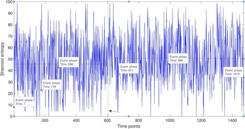
Figure 9 shows the plot of the time series of the FRP-based Shannon entropy of 19 moods of the major depression in all five phases of dose-reduction scheme. To detect the point where the most significant change in the time series occurs, a statistical change-point detection method (Killick et al. 2012) was used, where the chosen statistic was the mean. The change-point detection method identified the location at time point = 605 (the vertical line indicated with the arrow in Figure 9), which is in Phase 3, where the gradual reduction in the antidepressant dosage was carried out. The use of the time series of the fuzzy entropy of the FRPs resulted in similar results. To test if the difference of the Shannon entropy values between two phases is statistically significant, the paired-sample t-test was carried out to test the null hypothesis that the difference of the Shannon entropy between two phases might have occurred randomly or by chance, where the results come from a normal distribution with mean being equal to zero. Because the two sequences in a paired t-test must be of the same length, the longer sequence was truncated to have the same length as the other. A significance level = 0.05 was chosen, and the computed p-values $<.05$ were obtained for all the tests, which rejected the null hypothesis at the 5% significance level, indicating the differences are not likely to occur by chance.

Figure 9. Time series of FRP-based Shannon entropy of 19 moods of the major depression in all five phases of dose-reduction scheme. Time for Phase 1, = 1-176; Phase 2 = 176-286, Phase 3 = 286-671, Phase 4 = 671-988, and Phase 5 = 988-1472. The vertical line (time = 605 in Phase 3 and indicated with the arrow) is the time point, which was determined by a change-point detection method, where the time series changes most abruptly.

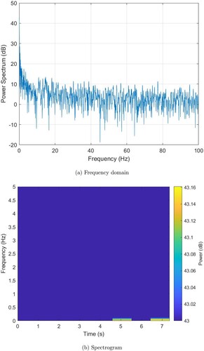
To further confirm the finding discovered in Figure 9 using the change-point detection, time-frequency analysis of the time series of the entropy of the FRPs of the data was applied. Figure 10 shows the frequency domain (Figure 10(a)) and spectrogram (Figure 10(b)) of the time series. The plot of the frequency domain of the time series, which was generated using the sampling frequency = 200 Hz, shows a sharp shift in power above 43 dB at frequency around 0.15 Hz. However, the frequency-domain plot does not provide any time information that indicates the order in which the transitions occurred. The spectrogram was then computed to reveal the frequency content of the signal varies with time. The spectrogram was computed over the 0 to 5 Hz band, with 0% overlap of data segments, and the content below the 43 dB power level was removed to visualize only the main frequency components and the transition durations and their locations in time. The plot shown in Figure 10(b) clearly shows the ordered presence of two transitions (yellow horizontal lines), which occurs first at the beginning of Phase 4 or end of Phase 3.

Figure 10. Time-frequency analysis of time series of FRP-based entropy for detecting critical transitions in major depression. (a) Frequency domain; (b) Spectrogram.

Discussion

The detected point at time = 605 as shown in Figure 9 is considered as a tipping point that indicates an anticipating critical transition of depression occurring in Phase 3 of the dose-reduction experiment. The main contribution to this sharp change point must be due to the reduction of antidepressants. In general, tipping points in complex systems can be considered as either early warnings of risks or indicators for positive changes (Scheffer et al. 2012). The tipping point detected in this study could not be confirmed as a sign of increasing or decreasing in positive or negative mood, but could be used as an early warning of a sudden transition in depressive symptoms, which needs urgent clinical attention for further diagnosis to provide possible new treatment strategy.

The complimentary use of the time-frequency analysis and spectrogram of the time series of the FRP entropy of the original data further confirmed the detection provided by the proposed method. The time-frequency analysis can only reveal potential sharp fluctuations in the frequency spectrum of the signal that can be considered as the presence of tipping points but cannot show particular times of the sharp changes. The spectrogram is then used to reveal the times of the frequency content of sharp shifts detected by the time-frequency analysis. Spectral analysis has also been recently applied for detecting changes in the sleep/wake cycle using actigraphy data to predict imminent transitions in mood episodes in bipolar patients (Kunkels et al. 2021).

Having presented the ability to combine multiple moods by means of an FRP, this case study opens an integrative method for detecting anticipating critical transitions in major depression. Studies on nonlinear time-series analysis and semantic expression of mental health have been set apart from each other. However, connection of these two areas can open doors to new perspectives. There is complementarity in the two analyses. The transformation of multiple mood scales into ordered data creates a measure of dynamics in mood changes in terms of the fuzzy recurrence entropy, and the sequence of such entropy values can discover tipping points of depression. A smart combination of methods may therefore enhance the power for predicting critical transitions in multi-dimensional data.

A previous study using the same data reported in Wichers and Groot (2016) shows a critical shift around day 127, which is around the end of Phase 3. The shift was clinically confirmed as the participant and his psychiatrist decided to resume the use of antidepressants 36 days after the experiment (the participant restarted to take the antidepressants as he had experienced a new episode of depression after the medication was terminated). There is an implication that the use of the FRP-based entropy of recurrence dynamics coupled with the statistical method for change-point detection and time-frequency analysis can detect an EWS.

In summary, results found in this study provide a discovery of an EWS that indicates the imminent development of a new episode of depression found after the stopping of antidepressant drug, which was clinically confirmed from a previous study about the detection of the vulnerability (Kossakowski et al. 2017). In comparison with a recent study using the same data (Pham 2020b) and as having mentioned earlier, this study considered 19 momentary moods on an individual basis, while the other explored 12 momentary moods that are combined into main 5 mental states (negative, positive, unrest, worrying, and suspicious) using fuzzy recurrence plots as features for tensor decomposition. The purposes of the two studies are different. This study aimed to investigate EWSs among the 5 experimental phases of the antidepressant reduction process. The other attempted to visualize differences among the 5 mental states in the 5 experimental phases.

Once again, sharp shifts in time series represent so-called critical transitions preceded by ‘tipping points’ (Scheffer et al. 2009). A tipping point is also considered as a feedback for an imminent transition toward an alternative state when a critical point has just passed (Angeli et al. 2004). In comparison with the study reported in Wichers and Groot (2016), the time points having the most significant change in the time series shown in the current results (Figures 9 and 10) appear to agree with the tipping point shown in the autocorrelation and variance results obtained from the previous report, where the critical transition detected from both methods is around the end of Phase 3. However, the proposed method detected the critical transition without manual analysis, thus illustrating its advantage over the other one. Furthermore, although the proposed method was applied to a case study of a personalized depression, the algorithm can be directly utilized or conveniently modified to detect critical transitions that can be signs of potential gains or losses in other multi-dimensional nonlinear dynamic systems in life sciences.

Conclusion

The concepts of fuzzy recurrence plots and their entropy measures have been addressed and found useful for studying the effect of dose reduction in a subject with major depression. The construction of fuzzy recurrence plots of the depression time series is feasible while the construction of the hard recurrence plots cannot be done. This shows an advantage of the performance of fuzzy recurrence plots. The proposed approach allows an effective integration of questionnaire-based data of many different mood states for data analytics that analyzes multiple sources of raw information to discover early warning signals about the mental behavior under study.

The results have demonstrated that the measure of entropy by the analysis of recurrence in time series has the potential to identify early signs of relapse on major depression. Particularly, in line with a hypothesis suggesting that major depression is a complex dynamic system (Cramer et al. 2016), the proposed method of nonlinear dynamics was applied for studying the unique time-series data of a major depression that include a valid critical transition and required number of observations in advance of the transition for detecting an EWS. It is of interest to further validate the effectiveness of the proposed approach when more depression data become publicly available. If the proposed approach can be proved rigorous, it will open a new door to the development of depression treatment and personalized medicine for depression, which is based on the hypothesis that specific biological or genetic variants of individuals can be predictive of specific treatment response.

Data availability statement

This third-party dataset is publicly available at the repository location: http://osf.io/j4fg8.

Disclosure statement

The author declares no competing interests.

Software availability statement

Matlab codes and data implemented in this study are publicly available at the author's homepage: https://sites.google.com/view/tuan-d-pham/codes.

References

- Angeli D, Ferrell JE, Sontag ED. 2004. Detection of multistability, bifurcations, and hysteresis in a large class of biological positive-feedback systems,. Proc Natl Acad Sci USA. 101:1822–1827.
- Bezdek JC. 1981. Pattern recognition with fuzzy objective function algorithms. New York: Plenum Press.
- Bos EH, De Jonge P. 2014. ‘Critical slowing down in depression’ is a great idea that still needs empirical proof. Proc Natl Acad Sci USA. 111:E878.
- Cramer Angélique OJ, van Borkulo CD, Giltay EJ, van der Maas HLJ, Kendler KS, Scheffer M, Borsboom D, Branchi I. 2016. Major depression as a complex dynamic system. PLoS ONE. 11:e0167490.
- Eckmann JP, Kamphorst SO, Ruelle D. 1987. Recurrence plots of dynamical systems. Europhys Lett. 4:973–977.
- Killick R, Fearnhead P, Eckley IA. 2012. Optimal detection of changepoints with a linear computational cost. J Am Stat Assoc. 107:1590–1598.
- Kossakowski JJ, Groot PC, Haslbeck JMB, Borsboom D, Wichers M. 2017. Data from ‘Critical slowing down as a personalized early warning signal for depression’. J Open Psychol Data. 5:1.
- Kunkels YK, Riese H, Knapen SE, Riemersma–van der Lek RF, George SV, van Roon AM, Schoevers RA, Wichers M. 2021. Efficacy of early warning signals and spectral periodicity for predicting transitions in bipolar patients: an actigraphy study. Transl Psychiatry. 11:350.
- Marwan N, Carmenromano M, Thiel M, Kurths J. 2007. Recurrence plots for the analysis of complex systems. Phys Rep. 438:237–329.
- Olthof M, Hasselman F, Strunk G, van Rooij M, Aas B, Helmich MA, Günter S, Lichtwarck-Aschoff A. 2020. Critical fluctuations as an early-warning signal for sudden gains and losses in patients receiving psychotherapy for mood disorders. Clin Psychol Sci. 8:25–35.
- Pham TD. 2016. Fuzzy recurrence plots. EPL. 116:50008.
- Pham TD. 2020a. Fuzzy recurrence entropy. EPL. 130:40004.
- Pham TD. 2020b. The recurrence dynamics of personalized depression, Proceedings Australasian Computer Science Week (ACSW' 20); New York, NY, USA: ACM. p. 8.
- Scheffer M, Bascompte J, Brock WA, Brovkin V, Carpenter SR, Dakos V, Held H, van Nes EH, Rietkerk M, Sugihara G. 2009. Early-warning signals for critical transitions. Nature. 461:53–59.
- Scheffer M, Carpenter SR, Lenton TM, Bascompte J, Brock W, Dakos V, van de Koppel J, IA van de Leemput, Levin SA, van Nes EH, Pascual M, Vandermeer J. 2012. Anticipating critical transitions. Science. 338:344–348.
- van de Leemput IA, Wichers M, Cramer Angélique OJ, Borsboom D, Tuerlinckx F, Kuppens P, van Nes EH, Viechtbauer W, Giltay EJ, Aggen SH, Derom C, Jacobs N, Kendler KS, van der Maas HLJ, Neale MC, Peeters F, Thiery E, Zachar P, Scheffer M. 2014. Critical slowing down as early warning for the onset and termination of depression. Proc Natl Acad Sci USA. 111:87–92.
- Wen H, Ciamarra MP, Cheong SA. 2018. How one might miss early warning signals of critical transitions in time series data: A systematic study of two major currency pairs. PLoS ONE. 13:e0191439.
- Wichers M, Groot PC. 2016. Critical slowing down as a personalized early warning signal for depression. Psychother Psychosom. 85:114–116.
- Zadeh LA. 1965. Fuzzy sets. Inf Control. 8:338–353.
- Zadeh LA. 1971. Similarity relations and fuzzy orderings. Inf Sci. 3:177–200.