An Evaluation of College Students’ Perceptions of Statisticians

Abstract

The widely used Draw a Scientist Test was revised to focus on statistics and 110 Elementary Statistics students were asked to draw a statistician. In addition, to better understand students’ drawings and have some relative comparison, 173 College Algebra students were asked to draw a mathematician. A detailed analysis of students’ images and students’ demographic information was conducted using descriptive statistics, categorical data analysis, logistic regressions, and hierarchical cluster analysis. Results showed that students tend to perceive statisticians and mathematicians as primarily White and male. However, female students were more likely than male students to draw a female statistician and mathematician. Two themed clusters emerged from the hierarchical cluster analysis for both the math and statistics students. We discuss the implications of the results for teaching and future research.

KEYWORDS:

• Draw a mathematician
• Draw a scientist
• Draw a statistician
• Gender differences
• Statistics
• STEM

1 Introduction

There has been a vast amount of research on gender and underrepresented minority group disparities in K-12 and college mathematics and science achievement and participation. Potential explanations for why outcomes favor males and White students (with the exception of Asian students) have included motivational differences, differences in strategy use, metacognitive differences, poor social support, socio-economic status, and stereotype threat (Carr and Jessup 1997; Jacobs 2005; Brown et al. 2016; Witherspoon and Schunn 2020; Pilotti 2021). Although the gender gap in achievement and enrollment has decreased in some sciences such as chemistry, and even disappeared in the biological sciences, the gap remains prominent in mathematics and in other sciences such as physics, computer science, and engineering (National Science Foundation, 2021). This is particularly true for more advanced degrees. For minority students, specifically Black and Latino/Hispanic students, a similar, but wider gap exists by area of STEM study. Furthermore, this disparity is compounded for minority women (National Science Foundation, 2021).

1.1 Gender and Racial Group Differences in Statistics Achievement and Participation

Less is known about gender and underrepresented racial group disparities in performance and participation in statistics and related fields such as data science and biostatistics. This is, in part, because so many U.S. progress reports on majors and degrees awarded by gender and racial status combine mathematics and statistics for analyses. However, statistics is quite different from mathematics in its approach, expectations, and conclusions and should be evaluated as its own area of study (Rossman et al. 2006). A thorough understanding of the role of gender and race/ethnicity in statistics performance and participation is essential given that, in the last decade, there has been a huge increase in the need for individuals who can organize and analyze the vast amount of data that is being collected. This constant influx of data has put statistics, biostatistics, and data science at the forefront of coveted majors and careers. For example, Forbes listed statistics as one of the 15 most valuable college majors (Forbes Magazine 2020). From 2016 to 2020, Glassdoor and Forbes listed data scientist as one of the Best Jobs in America with a 28% demand increase for data scientists in 2020 (Columbus 2017; Berkeley School of Information 2020; Glassdoor 2020). Thus, the need to recruit and retain diverse talent with data analytics skills has become crucial for providing varied perspectives, insights, and approaches to data analysis and statistical problem-solving needs in order to successfully and creatively evaluate the constant stream of data being accumulated.

1.1.1 Gender and Racial Disparities in Statistics Achievement

A search for peer-reviewed journal articles on gender differences in statistics achievement led to varying findings. At the college level, some research documented no gender differences in course grade among students taking undergraduate statistics (Woehlke and Leitner 1980; Buck 1985; Es and Weaver 2018), others found results in favor of women (Brooks 1986), while others found results in favor of men (Susbiyanto et al. 2019). A meta-analysis of 18 empirical studies showed that men outperformed women on college statistics course examinations, but women outperformed men in the course overall; gender differences in favor of women were more evident in business statistics courses than in psychology or education statistics courses (Schram 1996). Similar varying findings are reported in high school statistics. Saidi and Siew (2019) found that men outperformed women on a test of Central Tendency; Batanero, Merino, and Díaz (2003), in contrast, found no gender differences in high school students’ understanding of central tendency.

We searched extensively for research on racial disparities in statistics achievement. The research was limited to reports of racial disparities in participation, which are discussed below. There is little guidance from this research, however, regarding when and why these racial disparities in statistics participation begin and how they are linked to performance in statistics classes and programs.

1.1.2 Gender and Racial Disparities in Statistics Participation

There is evidence of gender and racial group disparities in participation in data professional occupations. A recent report documented that less than 17% of data analytics jobs are filled by women and 12% are filled by African Americans (4%) and Hispanics (8%) (Boas 2020; Dosad 2020). A second report indicated that just less than 30% of statistics related occupations are held by women (Boas 2020).

Understanding potential causes for women and underrepresented minorities’ low participation in statistics is crucial given the increasing availability of data and, primarily, big data in the last decade and the increased need for statisticians, biostatisticians, and data science talent to analyze those data. The need to keep a robust pipeline of professionals to help answer critical questions in medicine, immigration, business, education, industry, and economics has become increasingly vital in today’s data-centered, technologically advanced, fast-paced, and highly connected world. Thus, the need to retain women and underrepresented minorities in statistics, biostatistics, and data science is essential for continued progress in moving forward to use data to address the world’s problems. For example, in her book, Invisible Women: Exposing Data Bias in a World Designed for Men, Criado-Perez (2019) describes the disadvantages to women that result from biased data analyses that is primarily from a White male perspective. She explains that because data is mainly analyzed by men and for men, this creates a systematic bias and discrimination again women, causing them to be mistreated, misunderstood, and ignored in medical, industry, and technological research and innovation.

In the present study, students’ perceptions of a statistician were of interest to us. This is because of the well-established link between student perceptions and their retention and performance in academics (Songsore and White 2018). We were eager to understand the image college-aged students have of a statistician and the role of students’ gender and race/ethnicity on these mental images.

1.2 Student Perceptions of Statisticians

Student perceptions of their courses and learning environments are important because they impact their motivation, confidence, participation, enrollment, choice of major, and achievement (Bodzin and Gehringer 2001; Marx and Roman 2002). For example, mathematics and statistics students who perceive that they belong are more likely to pursue and apply mathematics and statistics in the future (Schau and Emmioğlu 2012; Tellhed, Bäckström, and Björklund 2017), and this perception and its implications is especially impactful for women (Burns and Lesseig 2017). The perception that one belongs occurs when an individual sees themselves as “fitting in” or as a representative/belonging member of a field. This perception of belonging, among students, has been linked to motivation, persistence, and engagement in academics (Goodenow 1993; Stout and Tamer 2016). The impact of belonging on enrollment and participation is particularly influential for students who are underrepresented in a field of study and for students about whom negative stereotypes exist (Steele 1997; Murphy et al. 2020). Stereotypes can hinder students’ perceptions of belonging.

1.2.1 Stereotypes and Stereotype Threat

For more than two decades, research has supported the notion that stereotypes induce psychological processes that meddle with an individual’s performance, boosting or impeding abilities according to the nature of the stereotype. The effects of stereotype threat have been repeatedly observed in mathematics performance (Spencer, Steele, and Quinn 1999; Good, Aronson, and Harder 2008; Picho and Schmader 2018) and documented as a contributing factor to gender and racial disparities in achievement and participation in mathematics. Those who experience stereotype threat in mathematics or hold the culturally upheld stereotype that White men are biologically predisposed to the subject, and that women and minorities are not mathematicians or suited for mathematics, experience a decreased sense of belonging to the mathematics community. This decreased sense of belonging leads to lower grades in mathematics courses and decreased intention to pursue mathematics in the future (Rattan, Good, and Dweck 2012). Students who identify themselves as being dissimilar to the prominent stereotypes of a field have been found to be less interested in the field (Lewis, Anderson, and Yasuhara 2016). If women and underrepresented minorities in statistics courses endorse the same stereotypes that are reported in mathematics and cannot find salient characteristics of themselves in the mental images that they have of a statistician, this will keep them from majoring and pursuing careers in statistics (Lewis, Anderson, and Yasuhara 2016).

The present study is novel in that it evaluates students’ perceptions by evaluating the mental image college-aged students have of statisticians and the role of student gender and race/ethnicity on these perceptions. Understanding students’ drawings of a statistician as related to their own race and gender provides us with information about what students believe a statistician looks like, but also gives us some insight into students’ perceptions of their own fit as a statistician and some understanding of their endorsement of common stereotypes. Understanding these perceptions, which are malleable and can shift based on situational cues (Kiefer and Sekaquaptewa 2007), is a necessary prerequisite for follow-up studies evaluating the link between gender and race/ethnicity, perceptions, achievement, and enrollment in statistics and for studies on interventions and efforts to modulate negative stereotypical perceptions and increase the retention of women and minorities in statistics.

2 Draw a Scientist Test

The Draw a Scientist Test (DAST), the test administered in the present study, is a well-known instrument that has been used to assess K-12 and college level students’ perceptions of a scientist (Thomas, Henley, and Snell 2006). The test was first developed by Chambers (1983), who administered to the test to nearly 5000 elementary aged children. Since then, it has been used in numerous studies to assess students’ perceptions of a scientist. A meta-analysis by Miller et al. (2018) provides a summary of five decades of DAST studies. The authors reviewed 78 studies ($N=20,860$; grades K-12) and found that students’ drawings depicted female scientists more often in later decades, but less often among older children. This suggests that students’ depictions of scientists have become more gender diverse over time, but that students become increasingly likely to associate scientists with males as they grow older. These drawings tend to depict scientists as White males (Finson 2002). The same pattern of the stereotypical White male scientist has been found among college students completing the DAST (Thomas, Henley, and Snell 2006).

The test has been extended and used to study students’ perceptions of mathematicians as the Draw a Mathematician Test (DAMT). The general trend of drawings in these studies is similar to what has been found using the DAST. Younger children are more likely to draw a female mathematician and as a teacher, likely because their source of learning math is from their teacher, and most elementary school teachers are female (Rock and Shaw 2000). As students progress through school and reach middle and high school, fewer students draw mathematicians as teachers and as females (Picker and Berry 2000; Aguilar et al. 2016). These images tend to be of balding and bearded Caucasian males with glasses. Even among college students, drawings of mathematicians tend to be male and male students are more likely to draw male mathematicians (Thomas, Henley, and Snell 2006; Piatek-Jimenez, Nouhan, and Williams 2020).

No version of the test, however, has been used to study student perceptions of statisticians. Ours is the first study to apply the test as a Draw a Statistician Test. The goal of the present study was to understand students’ perceptions of statisticians and how students’ gender and race play a role in those perceptions. To better understand those perceptions and have some relative comparison, we also collected data from mathematics students using the DAMT. Most of the studies using the DAST and DAMT have scored students’ tests for demographic and defining characteristics and have presented those results as descriptive statistics. We use categorical data analysis, text analysis, and hierarchical clustering to understand and compare student drawings within and between classes, presenting a more rigorous and novel analysis.

3 Method

3.1 Participants

We administered the Draw a Statistician Test to Elementary Statistics students and the Draw a Mathematician Test to College Algebra students on the first scheduled class of the Fall semester. Students were undergraduates enrolled at an R2 university in Georgia. Professors allowed the study and left the classroom during the duration of the test to minimize any internal biases. Although most classes did see their professors briefly (less than 3 min) before completing the test, our goal of collecting data on the first class of the semester was to minimize the role of demographics and physical characteristics of instructor on student responses.

One hundred and ten students in four sections of the Elementary Statistics course participated, including 74 women and 36 men. Three sections of the course were taught by a White male; one section of the course was taught by a White female. Seventy five (68%) of students identified as White, 15 (14%) of students identified as Black, 10 (9%) of students identified as Latino, 7 (6%) of students identified as Asian, 1 (1%) of students identified as Middle Eastern, and 2 (2%) of students did not report their race. Students were, on average, 20 years old with a standard deviation of 4 years.

One hundred seventy-three students in the College Algebra course participated including 69 women and 99 men; 5 students did not report their gender. One section of the course was taught by an Asian male, three sections were taught by white females, and one section was taught by a white male. Eighty-eight students (51%) identified as White, 54 (31%) of students identified as Black, 17 (10%) of students identified as Latino, 10 (6%) of students identified as Asian, and 4 (2%) of students did not report their race. Students were, on average, 20 years old with a standard deviation of 6 years.

3.2 Materials and Procedures

Students at the university are required to fulfill their general education requirements for their undergraduate degree; two options for courses include Elementary Statistics and College Algebra. Study materials administered to the students were identical except that the word statistician was replaced with mathematician for the College Algebra students. The test, with the instructions provided to the students, can be found in Appendix A.

Students were first asked to draw a Statistician/Mathematician doing statistics/mathematics. On a different page, students were then asked to report the gender, race, and age of the mathematician or statistician that they drew. Students were then asked to explain their drawing. Finally, students were asked to report their own gender, race, and age. Informed consent was collected from participants and the study was conducted in compliance with the authors’ Institutional Review Board.

4 Results

4.1 Descriptive Statistics and Categorical Data Analysis

Our Draw a Mathematician and Draw a Scientist test as shown in Appendix A was created, assessed, and scored using the work by Chambers (1983) and the Draw a Scientist Checklist and Rubric (Finson, Beaver, and Cramond 1995; Farland-Smith 2012). A graduate student scored the demographic information and evaluated the drawings for notable characteristics that were present in the drawings using guidelines for characteristics scored in Chambers (1983) and the Draw a Scientist Checklist and Rubric (Finson, Beaver, and Cramond 1995; Farland-Smith 2012). This included appearance: glasses, messy hair, and mood (happy and smiling or not) and location and activity, such as if the individual is in a lab or office, or if a desk, computer, whiteboard, or calculator was depicted. These characteristics of appearance, location, and activity are important and traditionally evaluated for DAST and DAMT studies because they provide additional context for the drawings beyond students’ reporting of the race and gender of the drawing. For the present study, these characteristics in the drawings were evaluated as part of the hierarchical cluster analysis. A second rater randomly selected and scored 50 of the Draw a Mathematician tests and 50 of the Draw a Scientist tests; interrater agreement as assessed by Cohen’s kappa was 0.95.

4.1.1 Analysis of Statistics Classes using the Draw a Statistician Test

Data were analyzed using SAS 9.4. We found that 71 of the drawings were of men statisticians (65%) and 35 were of women (32%) (4 pictures did not have a reported gender). In terms of race, 81 of the drawings were of White statisticians (74%), 10 (9%) were of Black statisticians, 4 (4%) were of Asian statisticians, and 2 (2%) were of Latino statisticians (13 pictures did not have a reported race). The average age of the drawn statistician was 38 years old with a standard deviation of 11 years. In addition, 65 (59%) of the drawings were of White males and 25 (23%) were of White females. Seven (6%) were of Black females, 4 (4%) were of Black males, and 3 (3%) were of Asian males.

We were interested in whether self-reported gender of the student was related to reported gender of the statistician. Figure 1 breaks down the data by gender.

Fig. 1 Student gender by gender of statistician in drawing.

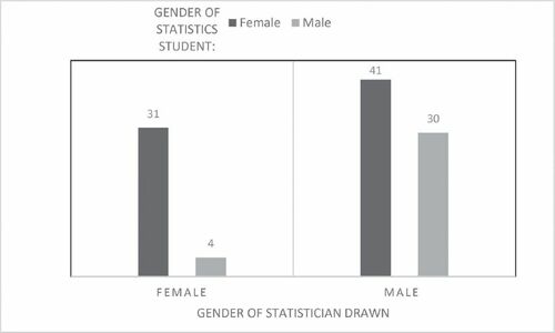
A chi-squared test of independence was conducted to determine whether female or male students were more likely to draw a female or male statistician. The results indicated that females were more likely than males to draw a female statistician, ${\chi }^2$ ($df=1,n=106$) = 10.22, p < 0.001. Only 12% of male students drew a female statistician; 43% of females drew a female statistician. Overall, students were more likely to draw a male statistician. (Four students did not report the gender of their statistician and were dropped from analysis to avoid low expected chi-square cell counts.)

A chi-squared test of independence and Fisher’s exact test were conducted to determine whether gender of the student was linked to race of statistician drawn. The results indicated that these variables were not related, ${\chi }^2$ (3, 106) = 1.35, $p=0.93$ and Fisher’s Exact Test p = 0.92. We also examined if race of the student was related to race of statistician drawn, using a chi-square test of independence. Results indicated that they were related: ${\chi }^2$ (20, 110)= 50.94, p = 0.01. Figure 2 breaks down the data by race.

Fig. 2 Student race by race of statistician in the drawing.

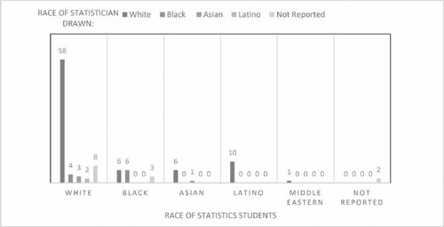
Because the statistical contingency table had some cells with expected values less than 5 (even with not reported values removed), we also report Fisher’s Exact test for a two tailed test, $p=0.01$. Results from Fisher’s Exact test indicated that most students drew a White statistician and this was particularly true for the White students (77%), Asian students (85%), Latino students (100%), and Middle Eastern students (100%). Black students were equally likely to draw a Black and White statistician.

Finally, the correlation between students’ age and age of the drawn statistician was not statistically discernable (not statistically significant), $r=-0.11$, p = 0.25.

4.1.2 Analysis of Mathematics Classes using the Draw a Mathematician Test

We found that 100 of the drawings were of male mathematicians (58%) and 58 were of female mathematicians (34%) (15 pictures did not have a reported gender). In terms of race, 108 (62%) of the drawings were of a White mathematician, 21 (12%) were of a Black mathematician, 11 (6%) were Asian mathematicians, 4 (2%) were of a Latino mathematician, and 1 (0.59%) was a mixed-race mathematician (28 pictures did not have a reported race). The average age of the drawn mathematician was 37 years old with a standard deviation of 13 years. In addition, 85 (54%) of the drawings were of White males and 33 (21%) were of White females. Eleven (7%) were of Black females, 6 (4%) were of Black males, and 6 (4%) were of Asian males.

We were interested in whether self-reported gender of the student was related to reported gender of the mathematician. Figure 3 breaks down the data by gender.

Fig. 3 Student gender by gender of mathematician in drawing.

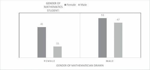
A chi-squared test of independence was conducted to determine whether female or male students were more likely to draw a female or male mathematician. The results indicated that females were more likely than males to draw a female mathematician, ${\chi }^2$ (1,156) 6.13, p = 0.01. Only 24% of male students drew a female mathematician; 44% of females drew a female mathematician. Overall, students were more likely to draw a male mathematician. (20 students did not report their own gender and gender of their mathematician and were dropped from analysis to avoid low expected chi-square cell counts.)

A chi-squared test of independence and Fisher’s exact test were conducted to determine whether gender of student was linked to race of drawn mathematician. Results suggested these variables are not related, ${\chi }^2$ (1, 156) 2.00, p = 0.73 and Fisher’s Exact Test p = 0.16. We also examined if race of the student was related to race of drawn mathematician using a chi-square test of independence, and results indicated it was: ${\chi }^2$ (20, 173) 56.34, p < 0.001. Because of several cells with expected values less than 5, we also report Fisher’s exact test, p < 0.001. Figure 4 breaks down the data by race.

Fig. 4 Student race by race of mathematician in the drawing.

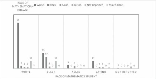
Most drawings were of a White mathematician. Except for nine students, all the White students drew a White mathematician. Results indicated that most students (who reported the race of their mathematician) drew White mathematicians and this was particularly true for the White students (88%). Other races also drew mostly White mathematicians including Asian students (50%) and Latino students (65%). Black students drew White mathematicians 43% of the time; they drew Black mathematicians 33% of the time. Non-White students in this sample, compared to the statistics students, were more likely show variability in the race of their drawings. One interesting finding was that the second most common drawing after a White mathematician was a mathematician that corresponded to the students’ own race. For example, Asian and Black students were most likely to draw a White mathematician, but after that, Asian students drew an Asian mathematician and Black students drew a Black mathematician.

Finally, the correlation between students’ age and age of the drawn mathematician was not statistically discernable, $r=-0.06,p=0.46$.

4.2 Hierarchical Cluster Analysis

4.2.1 Our Approach to Hierarchical Cluster Analysis

Hierarchical cluster analysis (HCA) was used to partition the students from Elementary Statistics and College Algebra into homogeneous groups (James et al. 2017). HCA, while a common clustering method, is but one of several existing methods that can be used for cluster analysis. For example, k-means clustering is also a commonly used method available in most modern statistical software packages. The main advantages of using HCA over k-means are twofold. First, k-means requires the researcher to specify the number of clusters to be fit a priori, which is somewhat limiting considering a primary goal of cluster analysis is to uncover a clustering structure. Second, HCA produces a useful graphic of the clustering process called a “dendrogram” which can be useful in further exploring relationships between observations regardless of the number of variables used (Hastie, Friedman, and Tisbshirani 2017). This contrasts with k-means, which can also produce a graphical representation of the clustering solution, but only up to three variables. Further, as the variables in our study to be used for clustering are all binary, Everitt et al. (2011) recommend utilization of HCA over k-means. Given this and given the straightforward implementation of HCA in statistical software, its usage was justified in the present study.

Agglomerative or “bottom-up” hierarchical clustering is a process which clusters most similar observations together in a stepwise manner until all observations are contained in the same cluster (Rencher and Christensen 2012). Step one of this process begins with each of the n observations; in this case each student response is its own “cluster” and a pairwise similarity or dissimilarity measure is calculated for each pair of observations (Rencher and Christensen 2012). The pair of observations most similar to each other are clustered together such that there are now n – 1 observations, and then the process moves to step two. Note, because we are starting at step two there will now exist clustered observations, and one must choose a method by which pairwise similarity or dissimilarity are calculated for such entities. These methods are referred to as “linkages” and are not an arbitrary choice as different linkages commonly result in different clustering solutions (James et al. 2017). There are three commonly used linkages: complete, single and average (Rencher and Christensen 2012). Complete linkage computes all pairwise dissimilarities or similarities between points in existing clusters and joins those with the minimum pairwise dissimilarities or maximum similarities (Everitt et al. 2011). Single linkage also calculates all pairwise dissimilarities or similarities between points in existing clusters, but then calculates the maximum pairwise dissimilarity or minimum similarity and joins those with the minimum or maximum of those values, respectively (Everitt et al. 2011). Finally, average linkage joins those two clusters whose average dissimilarity or similarity is either minimum or maximum, respectively. Clearly, the choice of linkage is not arbitrary, and thus all three of these commonly used methods were considered in order to determine the most optimum clustering solution.

Readers are directed to Charrad et al. (2014) for an overview of 30 different fit indices for cluster analysis. Each of these indices will give an indication as to the “best” fitting number of clusters. If a majority of indices agree upon a particular solution, then this is taken to be the best fitting solution (Charrad et al. 2014). In addition to these measures of internal validity, it is also important to consider cluster stability. Cluster stability refers to how consistently the same clusters appear after removing one variable at a time compared to the original clustering solution (Datta et al. 2008). More specifically, when assessing cluster stability, one variable is removed at a time, and a geometric property is recorded for the clustering solution sans that particular variable. This process occurs for all variables used for clustering. Then, traditional clustering stability measures typically take the average of the geometric property recorded and compare it to the geometric property for the full clustering solution (Datta et al. 2008). The smaller the deviation between these two values implies a more stable clustering solution. Taking measures of internal validity, clustering stability, as well as contextual information into consideration when deciding upon an appropriate clustering solution is a pragmatic approach (Lanza, Tan, and Bray 2013).

Our variables used for performing clustering were: student gender (a value of “1” denotes a male and a value of “0” denotes a female), student race/ethnicity (a value of “1” denotes white and all other race/ethnicity responses are denoted by a “0”), gender of the drawn mathematician/statistician (the same convention used for student gender is used here), race/ethnicity of the drawn mathematician/statistician (again, the same convention used for student race/ethnicity is used here), the mood of the drawn mathematician/statistician (a value of “0” denotes happy and a value of “1” denotes any mood besides happy), as well as individual dichotomous dummy variables indicating the appearance and location/activity of the drawing, which included the presence of “messy” hair, glasses, a calculator, a whiteboard, desk, teaching, or a computer in the drawing of the mathematician/statistician.

The drawing test contained a section where comments could be given with regards to the drawn mathematician/statistician. These comments aided in the clustering process. To include them, an overall text analysis was performed where common words (operationally, those which appeared two or more times) were grouped together by theme. New indicator variables were created which assumed a value of “1” if a student comment contained a keyword or keywords in a given theme and a value of “0” if the comment did not. While there were similarities between the mostly commonly occurring words, there were some differences between the two groups. Specifically, the statistics students tended to mention words relating to data and data analysis more than mathematics students. However, the nature of the keywords possessed a relatively high degree of similarity. A thematic analysis uncovered three broad themes across both classes: comments relating to physical appearance (e.g., gender, clothing, hair, etc.), teaching (e.g., classroom, whiteboard, etc.), and research/practicing the profession (e.g., equations, solving, analyzing, research, etc.). Table 1 shows keywords in each theme grouped by the two classes. These three themes were added in our cluster analysis. In total, 15 dichotomous variables were used to aid in identifying clustering solutions. Note, all variables were treated with equal weights.

Table 1 Keywords by theme for each class.

Mathematics			Statistics
Physical appearance	Teaching	Research	Physical appearance	Teaching	Research
Male	Teaching	Equations	Balding	Board	Analyzing
Smile	Chalkboards	Business	Clothes	Drawing	Calculator
Casual	Classroom	Calculators	Dress	Explaining	Chart
Happy	Whiteboard	Solving	Middle age	Professor	Computer
Curly Hair	Grade	Analyzing	Female	Students	Data
Outfit	Teacher	Professional	Glasses	Taught	Graph
Einstein	School		Guy	Teacher	Idea
Female	Students		Hair	Teaching	Paper
Wizard			Male	Whiteboard	Reading
Glasses			White	Class	Research
Dress					Thinking
White
Gender

One of the primary decisions which must be made prior to performing HCA is determining which measure of similarity should be used. Everitt et al. (2011) provide an overview of common similarity metrics. The metric chosen should be related to the type of data being analyzed. The variables included in the cluster analysis, as described above, are all dichotomous indicator variables. A measure used to define the similarity between two observations which contain only dichotomous indicator variables is called the $\varphi$ coefficient (Silge and Robinson 2017). For two observations, a 2 × 2 contingency table can be created as given in Table 2.

Table 2 A 2 × 2 contingency table for calculating the $\varphi$ coefficient.

		Observation j
		1	0	Total
Observation i	1	n11	n10	$n_{1.}$
	0	n01	n00	$n_{0.}$
	Total	$n_{.1}$	$n_{.0}$	n

Here, n₁₁ denotes the number of variables for observation i and j which both have “1” values. Similarly, n₁₀ represents the number of variables which observation i has a value of “1” and observation j has a “0” value. The other frequencies are defined in a similar fashion. Now, given this contingency table, the $\varphi$ coefficient between observation i and observation j is defined as(1) $${\varphi }_{i,j}=\frac{n_{11}{n}_{00}-n_{10}{n}_{01}}{\sqrt{n_{1.}{n}_{0.}{n}_{.0}{n}_{.1}}}.$$(1)

Note, this quantity is bounded between –1 and +1, as it is actually the Pearson correlation coefficient. In this analysis, and as is common in cluster analysis using the Pearson correlation coefficient as the measure of similarity, (1) was transformed to be on the [0,1] interval (Everitt et al. 2011). Denoted $d_{i,j}$, the measure of dissimilarity used in this analysis is given by(2) $$d_{i,j}=\frac{1-{\varphi }_{i,j}}{2}.$$(2)

Here, a number approaching 1 indicates a higher degree of dissimilarity between two observations. A number near 0 gives the opposite indication.

Using the statistical software program R (version 4.0.2), hierarchical clustering was performed (R Core Team 2020). As stated previously, all 15 variables used for clustering are indicator variables. One could reasonably justify the omission of the demographic variables from the HCA and use them after a clustering solution had been determined to explore demographic patterns and relationships among and within the clusters. However, since one could also reasonably assume that the responses to the demographic questions may have relationships with the other variables which in turn could provide more well-refined clusters, it was determined that their inclusion would be appropriate. To determine the appropriate clustering solution, we took into consideration internal validity measures (Connectivity, Average Silhouette Width, and the Dunn Index), a cluster stability measure (Average Distance between Means (ADM)), and contextual considerations such as number of observations in the smallest cluster (Datta et al. 2008). While the reader is directed to Datta et al. (2008) for a more thorough description of each of these measures, we provide a brief description of each metric. Generally, a “better” clustering solution would be one in which observations which are more similar or closer together geometrically are grouped together in the same cluster. Connectivity examines this phenomenon by examining the L-nearest neighboring points to each observation (with L typically being taken to be 10). If the Lth nearest neighbor to a given point is in the same cluster, a value of 0 is assigned. Otherwise, a value of 1/L is assigned. This occurs for every observation in the dataset and the sum of the values is called “Connectivity,” (Datta et al. 2008). The Average Silhouette Width takes a similar approach to Connectivity. If an observation is correctly clustered in cluster A, it would be expected that the dissimilarity between it and another observation in cluster A is small with respect to the dissimilarity between said observation and another observation in the nearest cluster, say cluster B (Rousseeuw 1987). That is to say, if observation i is “well-clustered” in cluster A, it has little dissimilarity from other observations in cluster A and has greater dissimilarity from observations clustered in B (Rousseeuw 1987). This value is bounded between –1 and +1 (like the correlation coefficient) with values closer to +1 indicating a “better” fit and values closer to –1 indicating the opposite. The Dunn Index “is the ratio of the smallest distance between observations not in the same cluster to the largest intra-cluster distance,” (Datta et al. 2008). If a clustering solution is of high quality, the largest intra-cluster distance would be small and the smallest inter-cluster distance would be big, therefore, implying that large values of the Dunn Index are preferrable to smaller values. Finally, ADM is the average distance between centroids of a given clustering solution removing one variable from the cluster analysis at a time. This measure of cluster stability is conceptually similar to Cook’s Distance, which is a commonly used measure of observation influence in regression analysis. With Cook’s Distance, a standardized value is obtained for each observation demonstrating the degree to which the estimated regression coefficients change with the omission of a specific observation. ADM examines a similar phenomenon by exploring how much individual variables can influence a clustering solution. Of note, while this general method of assessing cluster stability is commonly used, it is not the only method by which cluster stability can be evaluated. For example, one could randomly sample observations from the full dataset to obtain a smaller dataset and perform HCA. If the clustering solution obtained by the HCA on the smaller dataset is geometrically similar to the solution obtained by the full dataset, then this would indicate a stable solution (Mufti, Bertrand, and Moubarki 2005).

In these analyses, we considered two through eight class solutions as larger class solutions can contain small clusters which can be difficult to interpret. To calculate the internal validity, the clValid function within the clValid package was used (Datta et al. 2008). For a proposed clustering solution, the function will calculate the internal validity measures. For each of the considered metrics besides Connectivity, the maximum value is taken to be the optimum clustering solution, whereas Connectivity is to be minimized (Datta et al. 2008). Then, the number of clusters which have the highest degree of agreement among the fit indices are taken to be the “best” solution. To calculate the cluster stability, the clValid function was also used to obtain the ADM values with smaller values suggesting a more stable clustering solution (Datta et al. 2008). Note, while the clValid function produces four stability measures, only ADM was used as the measure had to be computed manually for the mathematics class. The measures of internal validity and stability for each of the considered linkages are given by Tables 3 and 4 for the statistics and mathematics classes, respectively, as well as in Figures 5 and 6.

Fig. 5 Statistics class clustering fit indices.

Fig. 6 Mathematics class clustering fit indices.

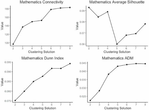
Table 3 Statistics Class Clustering Fit Indices.

Statistics Class HCA
		Index	2-Class	3-Class	4-Class	5-Class	6-Class	7-Class	8-Class
Average linkage	Internal validity	Connectivity	7.8548	10.8837	20.6369	48.3575	57.4794	81.0091	82.3282
		Dunn	0.2830	0.2830	0.2432	0.1510	0.1678	0.1708	0.1708
		Silhouette	0.2694	0.1580	0.0950	0.1706	0.1793	0.1804	0.1618
	Cluster stability	ADM	0.0596	0.1588	0.3260	0.4352	0.3635	0.4705	0.4424
	Minimum cluster size	n (%)	4 (3.64%)	1 (0.91%)	1 (0.91%)	1 (0.91%)	1 (0.91%)	1 (0.91%)	1 (0.91%)
Complete linkage	Internal validity	Connectivity	67.2996	80.4770	92.1643	102.8627	110.3373	113.0702	125.0040
		Dunn	0.0813	0.0852	0.0932	0.0987	0.1044	0.1048	0.1059
		Silhouette	0.1324	0.1080	0.1325	0.1486	0.1547	0.1524	0.1428
	Cluster stability	ADM	0.4801	0.6241	0.6875	0.7042	0.7185	0.7279	0.7550
	Minimum cluster size	n (%)	42 (38.18%)	16 (14.55%)	13 (11.92%)	13 (11.92%)	11 (10.00%)	4 (3.64%)	4 (3.64%)
Single linkage	Internal validity	Connectivity	3.3734	6.4024	9.5452	13.1631	15.8393	19.1349	22.5317
		Dunn	0.3426	0.3344	0.3297	0.2830	0.2830	0.2708	0.2708
		Silhouette	0.2557	0.1578	0.1217	0.0643	0.0377	0.0036	–0.0152
	Cluster stability	ADM	0.0325	0.0537	0.0511	0.0754	0.1021	0.1027	0.1171
	Minimum cluster size	n (%)	1 (0.91%)	1 (0.91%)	1 (0.91%)	1 (0.91%)	1 (0.91%)	1 (0.91%)	1 (0.91%)

Note: For the measures of internal validity and cluster stability, a greater number is preferrable to a smaller number except for Connectivity and ADM where the opposite is the case. Bolded values indicate the optimum value for a given metric.

Table 4 Mathematics Class Clustering Fit Indices.

Mathematics Class HCA
		Index	2-Class	3-Class	4-Class	5-Class	6-Class	7-Class	8-Class
Average linkage	Internal validity	Connectivity	6.9714	25.0210	25.0210	57.3778	59.4996	69.9778	91.2484
		Dunn	0.2265	0.1001	0.1001	0.0857	0.0857	0.0857	0.0857
		Silhouette	0.3253	0.2104	0.1188	0.1108	0.0903	0.0706	0.0792
	Cluster stability	ADM	0.0158	0.0176	0.0170	0.0200	0.0198	0.0289	0.0411
	Minimum cluster size	n (%)	3 (1.73%)	3 (1.73%)	2 (1.16%)	2 (1.16%)	2 (1.16%)	2 (1.16%)	2 (1.16%)
Complete linkage	Internal validity	Connectivity	96.7944	137.0567	149.5702	152.6214	178.2806	181.7333	182.9302
		Dunn	0.0752	0.0799	0.0849	0.0876	0.0917	0.0917	0.0942
		Silhouette	0.0928	0.0843	0.0890	0.0600	0.0680	0.0694	0.0781
	Cluster stability	ADM	0.0225	0.0283	0.0382	0.0430	0.0440	0.0446	0.0445
	Minimum cluster size	n (%)	74 (42.77%)	49 (28.32%)	23 (13.29%)	9 (5.20%)	9 (5.20%)	8 (4.62%)	3 (1.73%)
Single linkage	Internal validity	Connectivity	3.3873	6.7925	9.9575	13.6865	18.0238	21.9528	23.3817
		Dunn	0.2984	0.2503	0.2609	0.2554	0.2544	0.2544	0.2544
		Silhouette	0.3360	0.2803	0.2303	0.0672	0.0116	–0.0101	–0.0167
	Cluster stability	ADM	0.0149	0.0152	0.0154	0.0162	0.0162	0.0163	0.0170
	Minimum cluster size	n (%)	1 (0.58%)	1 (0.58%)	1 (0.58%)	1 (0.58%)	1 (0.58%)	1 (0.58%)	1 (0.58%)

Note: For the measures of internal validity and cluster stability, a greater number is preferrable to a smaller number except for Connectivity and ADM where the opposite is the case. Bolded values indicate the optimum value for a given metric.

For both classes, complete linkage was chosen as it provided more meaningful clustering solutions in terms of the minimum cluster size. Especially compared to single linkage, complete linkage tends to provide more “balanced” clusters (James et al. 2017). Single linkage, at each step in the agglomerative process, can tend to have points join one large cluster one at a time, which can result in substantially imbalanced clusters (James et al. 2017). For the statistics class, the best fitting solution was determined to be two clusters. Notice in Table 3 in the rows for complete linkage, Connectivity would suggest a two-cluster solution, and the Dunn Index and Average Silhouette Width seem to increase albeit incrementally with each additional class. The two-class solution was chosen because the majority of indices pointed to this solution. Further, a visual examination of Figure 5 shows the dendrogram for the statistics class with boxes enclosing the specific clusters. Based on this graphic, in addition to the metrics calculated in Table 3, it was deemed that the two-class solution was justified. In terms of cluster stability, one may be inclined to instead choose a clustering solution provided by average or single linkage as the ADM values for both are nearly uniformly less than those produced by complete linkage. This is a bit misleading, however, as nearly all the clustering solutions included a solution with a single observation.

For the mathematics class, a two-class solution was also chosen. Examining Table 4 in the rows associated with complete linkage, while the Dunn Index incrementally increases with each additional cluster, Connectivity and the Average Silhouette Width are firmly in the two-class solution in addition to having an interpretable minimum cluster size. Further, across all linkages, the two-class solution yielded the minimum ADM value, thus implying it is the most stable solution.

4.2.2 Statistics Class Analysis

To identify the predominate characteristics of each cluster, proportions of the analyzed variables were calculated and are given in Table 5. Characteristics in a cluster with a proportion greater than about 60% (more than half) were contributing factors to the cluster title. Figure 7 provides the complete linkage dendrogram for the statistics class.

Fig. 7 Dendrogram for statistics class.

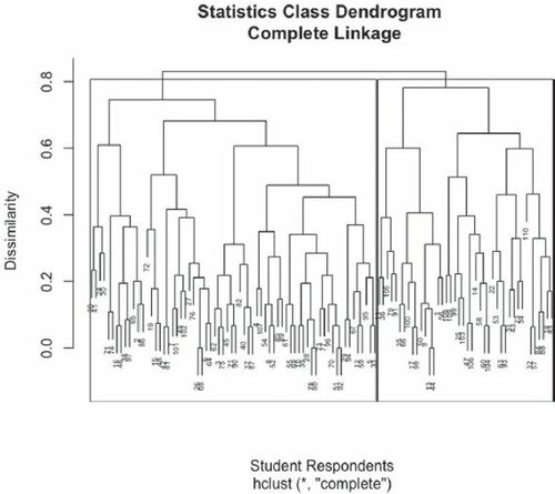
Table 5 Statistics class cluster variable proportions.

Cluster	White students	White females drawing
theme	drawing white	white males
	(unhappy) females	with whiteboards
N	42	68
% Male students	42.86%	26.47%
% White students	80.95%	60.29%
% Male drawings	30.95%	85.29%
% White/Caucasian drawings	69.05%	76.47%
% Drew glasses	21.43%	38.24%
% Drew calculator	9.52%	11.76%
% Drew whiteboard	35.71%	75.00%
% Drew desk	33.33%	16.18%
% Drew messy hair	14.29%	14.71%
% Drew computer	23.81%	8.82%
% Physical appearance comments	16.67%	33.82%
% Teaching comments	38.10%	32.35%
% Research comments	54.76%	23.53%
% Drew students	0.00%	4.41%
% Drew unhappy mood	66.67%	41.18%

In the cluster entitled, “White Females Drawing White Males with Whiteboards,” most of the students grouped in this cluster were female who drew White males. Further, 75% of the students in this group drew their statistician with a whiteboard, which indicates that they view a statistician as being primarily a teacher. In the cluster entitled, “White Students Drawing White (unhappy) Females” a predominate majority of the students were White and drew White female statisticians. In addition, many of the students in this cluster were females and included comments that suggested their statistician was involved in research.

4.2.3 Mathematics Class Analysis

Results of the hierarchical cluster analysis for the mathematics students is presented in Table 6, with Figure 8 presenting the dendrogram for this class. Characteristics in a cluster with a proportion greater than about 60% (more than half) were contributing factors to the cluster title in Table 6.

Fig. 8 Dendrogram for mathematics class.

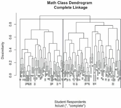
Table 6 Mathematics class cluster variable proportions.

Cluster	Drawings of white	Drawings by females
theme	male mathematicians	of happy, white
	who are unhappy	teachers at a whiteboard
N	99	74
% Male students	41.41%	37.84%
% White students	49.49%	52.70%
% Male drawings	67.68%	44.59%
% White/caucasian drawings	60.61%	64.86%
% Drew glasses	34.34%	9.46%
% Drew calculator	8.08%	1.35%
% Drew whiteboard	56.57%	97.30%
% Drew desk	21.21%	4.05%
% Drew messy hair	12.12%	24.32%
% Drew computer	7.07%	0.00%
% Physical appearance comments	55.56%	48.65%
% Teaching comments	37.37%	67.57%
% Research comments	33.33%	12.16%
% Drew students	1.01%	21.62%
% Drew unhappy mood	74.75%	39.19%

One cluster drew their mathematician as White and unhappy males (many of which were drawn by females and included whiteboards). The second cluster included drawings by females who drew their mathematician as White, happy teachers. It is interesting to note that this second cluster was comprised of mostly White female students who drew mostly female mathematicians (55%).

4.3 Comparison of the Mathematics and Statistics Students

To compare the mathematics and statistics students, we ran logistic regression models to obtain the odds ratios and odds of each model for each sample. The odds ratios were used to compare students within a class on their drawings; the odds, odds ratios, log odds, and their associated significance were used to compare how much more likely students in one class were to exhibit a particular characteristic in their drawings.

In the first model, we tested whether gender of student impacted gender of statistician/mathematician drawn. The odds of drawing a female statistician for the female students was 5.84 times the odds of drawing a female statistician for the male students. Specifically, the odds that a female draws a female statistician is 0.76 (31/41 from the chi-squared analysis; please see Figure 1) and the odds that a male draws a female statistician is 0.13 (4/30 from the chi-squared analysis; please see Figure 1).

The odds of drawing a female mathematician for the female students was 2.41 times the odds of drawing a female mathematician for the male students. Specifically, the odds that a female draws a female mathematician is 0.77 (41/53 from the chi-squared analysis; see Figure 3) and the odds that a male draws a female mathematician is 0.32 (15/47 from the chi-squared analysis; see Figure 3). The log odds associated with each group were discernable (p = 0.01 for the math students and p = 0.003 for the statistics students). Overall, females were more likely than males to draw a female statistician and mathematician. The odds ratio for the comparison of the groups was 2.42, suggesting that the effect of a female drawing a female in comparison to a male drawing a female was higher among the statistics students than mathematics students.

In a second model, we tested whether race of the student impacted race of statistician/mathematician drawn. Because 68% of the statistics students were White and 14% were Black, and because the other race categories were small, we examined whether race of student impacted race of statistician drawn. We chose to categorize race of statistician drawn at 1 White and 0 for everyone else because only 15% of the drawings were of non-White statisticians. For the statistics students, the odds of drawing a non-White statistician for the non-White students was 1.48 times the odds of drawing a non-White statistician for the White students (log odds discernable at p = 0.01). The same coding was used for the mathematics students because only 25% of the races in the pictures were non-White and 82% of the students in the class were White or Black. For the mathematics students, the odds of drawing a non-White mathematician for the non-White students was 3.62 times the odds of drawing a non-White mathematician for the White students (log odds discernable at p < 0.001). Overall, non-White students were more likely than White students to draw a non-White mathematician or statistician. The odds ratio of the comparison of groups was 0.41, suggesting that non-White mathematics students, compared to their statistics counterparts, were more likely than White students to draw a non-White image.

In a final set of models, we tested whether gender of student impacted race of statistician/mathematician drawn. The chi-square tests for each area of study indicated that these variables were not linked. The results of the logistic regression analysis also confirmed that the model was not statistically discernable.

5 Discussion

This is the first study to apply the DAST as a Draw a Statistician Test. The goal of the present study was to understand students’ perceptions of statisticians and how students’ gender and race play a role in those perceptions. To better understand students’ perceptions and have some relative comparison, we also collected data from mathematics students using the DAMT. We used categorical data analysis, text analysis, and hierarchical clustering to understand and compare student drawings within and between classes. We also used logistic regression to obtain odds ratios to compare whether the links between race and gender of drawing, student, and professor were discernable between groups.

We found, consistent with the research that we reviewed, that mathematics students see mathematicians as primarily White and male. Although students overall were most likely to draw a male mathematician, the chi-square and logistic regression results suggested that male students were more likely to draw a male mathematician and female students were more likely than male students to draw a female mathematician (44% of females drew a female mathematician).

Non-White mathematics students were more likely than White students to draw a non-White mathematician. One interesting finding for the mathematics students was that the second most common drawing after a White mathematician was a mathematician that corresponded to the students’ own race. For example, Asian and Black students were most likely to draw a White mathematician, but after that, Asian students drew an Asian statistician and Black students drew a Black statistician.

In this study, the first to examine students’ images of statisticians and the link between demographic variables and those perceptions, we found similar results among statistics students. Statistics students overall were more likely to draw a White male statistician. However, within gender, male students were more likely to draw a male statistician and female students were more likely than male students to draw a female statistician. In fact, 43% of females drew a female statistician. Thus, females were more open, than males, to the idea of a female statistician. This is an optimistic finding given the Women in Data Science organization (WiDS) initiative of “30 by 30” or having 30% of data scientists be women by the year 2030. There was a fair amount of female representation in the drawings by the females, suggesting that many females can see a statistician as being a female. This is important given reports of large gender disparities in favor of males in statistics related occupations (Boas 2020; Dosad 2020). However, this question emerges from our results: if females can see themselves as statisticians, then why are they not entering statistics related careers? One potential explanation for this disparity in representation in drawings and participation of females is that males’ perception that statisticians are primarily White males may indirectly impact the participation of women in statistics through the expectations and behaviors of males toward women (biases, discrimination, views of women’s capability, parenting expectations, double standards, bullying, harassment) as evidenced in other STEM fields (O’Connell and McKinnon 2021). We discuss this further below, but another explanation is that while statistics is becoming a subject more broadly studied in secondary education, many students come into their first statistics course in college with little experience with a statistics-specific teacher. Therefore, a possible explanation for this disparity in drawings and participation could be that a student might not have a fully formed image of what a statistician ought to look like and thus they chose to draw someone who looks like themselves when gaps in perceptions are present. A third explanation is that other factors may be playing a larger role than perceptions in keeping women from participating in statistics. Additional research is needed to understand the interacting cognitive, social, emotional, and motivational factors that may be contributing to this disparity in participation. Multilevel, longitudinal, and structural equation modeling are ideal techniques for studying which of many interacting variables are most important for participation and at what time.

Finally, there was no link between gender of the student and race of the statistician drawn. Non-White statistics students were more likely than White students to draw a non-White statistician. An interesting finding for the statistics students was that Black students were equally likely to draw a Black and White statistician. This was not the case for the other student race groups who mainly drew a White statistician.

The cluster analysis showed some interesting clusters. For the mathematics students, two clusters emerged from the data including “Drawings of White Male Mathematicians Who Are Unhappy” and “Drawings by Females of Happy, White Teachers at a Whiteboard.” In this second cluster, most of the drawings were of females (55%). These findings from the second cluster are parallel to those found by Rock and Shaw (2000) where elementary aged students drew female mathematicians as teachers. The first cluster aligns with the stereotype that mathematicians are White men. Both clusters were comprised of primarily females drawing White mathematicians.

Two clusters also emerged for the statistics students, one of which was “White Females drawing White Males with Whiteboards.” These females drew their statistician with a whiteboard, suggesting that they likely viewed their statistician as a teacher. A second cluster was that of “White Students drawing White (unhappy) Females. While statistics is becoming a subject more broadly studied in secondary education, many students come into their first statistics course in college with little experience with a statistics-specific teacher. Therefore, a possible explanation for this result could be self-projection, particularly because many of the students in this group were females. A student might not have a fully formed image of what a statistician ought to look like and thus they chose to draw someone who looked like themselves when gaps in perceptions were present. Individualized or focus group interviews with these clusters of students would provide insight into how and why they differ from the majority of students who view statisticians as White males.

5.1 Altering Student Perceptions with Relevant Role Models

Stereotypes can be detrimental for retention of women and minorities in college mathematics and statistics courses, which has led researchers to search for solutions on how to negate these negative effects. It becomes less likely that students will pursue careers in statistics and data science if their perception of data professionals fail to align with their beliefs about themselves (Goodenow 1993; Lewis, Anderson, and Yasuhara 2016; Murphy et al. 2020). Research shows that students’ career preferences and aspirations are linked to their views of who belongs in a particular occupation (Songsore and White 2018). In this study, understanding students’ drawings of a statistician or mathematician as related to their own race and gender provided us with information about what students believe a statistician or mathematician looks like and gave us perspective into students’ perceptions of their own fit as a statistician or mathematician and their endorsement of common stereotypes.

We found that females and minorities in statistics and mathematics courses see practicing statisticians and mathematicians as primarily White and male, a possible explanation for the gender and racial group disparities in participation in data professional occupations. However, student perceptions are malleable and can shift based on situational cues (Kiefer and Sekaquaptewa 2007). Ensuring that students see and interact with statisticians of different genders and ethnicities can allow students to see themselves reflected in those individuals (Lewis, Anderson, and Yasuhara 2016; Songsore and White 2018). This should, in turn, increase their perceptions of belonging and the likelihood of retaining them in statistics majors and careers (Lewis, Anderson, and Yasuhara 2016).

When it comes to statistics, or even the broader field of STEM, studies have investigated how environmental cues such as role models, media content, and cultural stigmas play a role in shaping one’s perceptions toward the subject. Research provides ample evidence that authority figures and role models influence thoughts and behaviors, whether that be in a positive or negative light. Previous studies have found that women’s leadership skills and self-evaluations are positively affected (Latu et al. 2013), negative self-perceptions are decreased, leadership aspirations are increased (Simon and Hoyt 2013), automatic gendered stereotyping is reduced (Dasgupta and Asgari 2004), and the effect of the gender-math stereotype threat on women’s math performance is reduced (Marx and Roman 2002) when working with a positive female role model.

A study by Haley, Johnson, and Kuennen (2007) examined the role of professor and student genders on student achievement in an introductory level business statistics course that was taught by economics faculty. The authors found that students taught by a professor of the opposite gender performed more poorly than students taught by a professor of the same gender. In line with this, Blackwell (1988) reported that the presence of Black faculty was the most statistically significant predictor of enrollment and graduation of Black graduate students. Both studies attest to the importance diversity of statistics faculty. This diversity can provide inclusive role models which, in turn, can alter students’ perceptions, retention, and success.

Countering negative stereotypes through media content has also been explored, especially given the abundance and availability of content in the modern age. One study found that women under gender-math stereotype threat selected counter stereotypical magazines with career material, rather than equally accessible beauty and home improvement magazines, to manage the threat they were under. This effect of selective exposure to counter stereotypical magazine content on women’s math performance was significantly moderated by feelings to relatedness to the female role models in the magazines. Specifically, for women who felt a sense of relatedness to the career role models, longer exposure time to the career magazine led to better math performance (Luong and Knobloch-Westerwick 2017).

Reinforcement of diverse and positive stereotypes, through contact with and exposure to various role models (i.e., teachers, professional statisticians or data scientists) appears to be a useful way to counteract stereotype threat’s effect on students’ perceptions and, in turn, achievement and participation.

5.2 Organizations and Programs that Provide Diverse Role Models

There are organizations and programs that support women and minority women in statistics and data science. Despite the current push in U.S. public schools to allow students to substitute Statistics for Algebra 2 in order to prepare students for the analytics skills needed for this data-rich world (Boaler and Levitt 2019), the time in which most students tend to take their first statistics course is in college. Providing the students in these courses, as early as possible, with women and minority women role models and mentors, can help mitigate any White, male dominated stereotypes associated with statistics. Some national organizations that provide support for women and women minorities include: Women in Data Science Conference (WiDS), a one day annual conference offered by Stanford University where women can learn about leading trends in data science and network with women mentors and peers: https://www.widsconference.org/. Another organization, Women in Machine Learning and Data Science (WiMLDS), supports and promotes women and women minorities who are studying or practicing machine learning or data science by providing them with workshops, networking events, and hackathons. Other programs include Girls who Code, that attempts to close the gender gap in programing: https://girlswhocode.com/ and Women in Big Data, which provides an online forum and events to attempt to increase the number of women and women minorities in big data https://www.womeninbigdata.org/.

6 Conclusion

This study showed that students tend to perceive statisticians as mostly White and male. Given the low percentage of women professionals in statistics and data science, efforts to increase women and women minority representation is important for supplying the talent to evaluate the abundant amount of data being collected. Although we included the mathematics students as a control group, an additional control group could be similarly aged individuals who are not attending college. A comparison group that includes individuals from a very different background can provide additional and unique insight on how statisticians are perceived. One limitation of this study is that students’ images of statisticians could not be linked to their course performance. Additional research needs to be done to study gender and minority differences in statistics performance, and the cognitive, motivational, and social factors that attenuate and amplify those differences. Research should also study students at various courses in their study of statistics to determine if, when, and why differences may emerge. Structural equation modeling and multilevel modeling can help with the analysis of mediating, longitudinal, and nested effects. A combination of quantitative and qualitative techniques can provide a thorough study of any gender and race disparities, allowing for effective and targeted intervention research to be conducted. Finally, research on the impact of stereotype threat on statistics achievement, perceptions, stereotype awareness and endorsement, motivation (including self-efficacy, expectancy-value), and retention should be conducted.

Appendix A:

Draw a Statistician Test

By participating in this survey, you are indicating that you understand that your responses are anonymous and will not be identified with you in any way and that you are at least 18 years old. If you do not wish to participate in the survey, please leave the survey blank.

In the space below, please illustrate your idea of a statistician doing statistics.

In the boxes below, please state the age, gender, and race of the statistician you have illustrated above.

Table

Age of statistician	Gender of statistician	Race of statistician

In the box below, please explain why you drew what you drew (for the outfit, any accessories, facial descriptors, background, or any additional objects).

Table

In the boxes below, please state your age, gender, and race.

Table

Your age	Your Gender	Your Race

References

- Aguilar, M. S., Rosas, A., Zavaleta, J. G. M., and Romo-Vázquez, A. (2016), “Exploring High-Achieving Students’ Images of Mathematicians,” International Journal of Science and Mathematics Education, 14, 527–548. DOI: https://doi.org/10.1007/s10763-014-9586-1.
- Batanero, C., Merino, B., and Díaz, C. (2003), “Assessing Secondary School Student’s Understanding of Average,” European Research in Mathematics Education III, 3, 1–9.
- Berkeley School of Information (2020), “What is Data Science?” Available at https://datascience.berkeley.edu/about/what-is-data-science/.
- Blackwell, J. E. (1988), “Faculty Issues: The Impact on Minorities,” The Review of Higher Education, 11, 417–434. DOI: https://doi.org/10.1353/rhe.1988.0013.
- Boaler, J., and Levitt, S. D. (2019), “Modern High School Math Should be about Data Science — not Algebra 2.” Los Angeles Times. Available at https://www.latimes.com/opinion/story/2019-10-23/math-high-school-algebra-data-statistics.
- Boas, L. V. (2020), “Diversity in Data Science: A Systemic Inequality How FAANG Companies are Dealing with this Structural Problem. Towards Data Science,” Ävailable at https://towardsdatascience.com/diversity-in-data-science-a-systemic-inequality-b97a0e953f6e.
- Bodzin, A., and Gehringer, M. (2001), “Breaking Science Stereotypes,” Science and Children, 38, 36–41.
- Brooks, C. I. (1986), “Female Superiority in Statistics Achievement,” Teaching of Psychology, 14, 45–46. DOI: https://doi.org/10.1207/s15328023top1401_13.
- Brown, P. L., Concannon, J. P., Marx, D., Donaldson, C. W., and Black, A. (2016), “An Examination of Middle School Students’ STEM Self-efficacy with Relation to Interest and Perceptions of STEM,” Journal of STEM Education, 17, 27–38.
- Buck, J. L. (1985), “A Failure to Find Gender Differences in Statistics Achievement,” Teaching of Psychology, 12, 100. DOI: https://doi.org/10.1207/s15328023top1202_13.
- Burns, H. D., and Lesseig, K. (2017), “Infusing Empathy into Engineering Design: Supporting Under-represented Student Interest and Sense of Belongingness,” in American Society for Engineering Education Annual Conference & Exposition, Columbus, Ohio.
- Carr, M., and Jessup, D. L. (1997), “Gender Differences in First-Grade Mathematics Strategy Use: Social and Metacognitive Influences,” Journal of Educational Psychology, 89, 318–328.
- Chambers, D. W. (1983), “Stereotypic Images of the Scientist: The Draw-a-Scientist Test,” Science Education, 67, 255–265. DOI: https://doi.org/10.1002/sce.3730670213.
- Charrad, M., Ghazzali, N., Boiteau, V., and Niknafs, A. (2014), “NbClust: An R Package for Determining the Relevant Number of Clusters in a Student,” Journal of Statistical Software, 61, 1–36. DOI: https://doi.org/10.18637/jss.v061.i06.
- Columbus, L. (2017), “IBM Predicts Demand For Data Scientists Will Soar 28% By 2020.” Available at https://www.forbes.com/sites/louiscolumbus/2017/05/13/ibm-predicts-demand-for-data-scientists-will-soar-28-by-2020/{\#}2f3902ea7e3b.
- Criado-Perez, C. (2019), Invisible Women: Exposing Data Bias in a World Designed for Men, New York: Abrams Press.
- Dasgupta, N., and Asgari, S. (2004), “Seeing is Believing: Exposure to Counterstereotypic Women Leaders and its Effect on the Malleability of Automatic Gender Stereotyping,” Journal of Experimental Social Psychology, 40, 642–658. DOI: https://doi.org/10.1016/j.jesp.2004.02.003.
- Datta, S., Datta, S., Pihur, V., and Brock, G. (2008), “clValid: An R Package for Cluster Validation,” Journal of Statistical Software, 25, 1–22.
- Dosad, M. (2020), “The Gender Gap in Data Analytics,” Available at https://www.harnham.com/us/the-gender-gap-in-data-analytics
- Es, C. V., and Weaver, M. M. (2018), “Race, Sex, and their Influences on Introductory Statistics Education,” Journal of Statistics Education, 26, 48–54. DOI: https://doi.org/10.1080/10691898.2018.1434426.
- Everitt, B. S., Landau, S., Leese, M., and Stahl, D. (2011), Cluster Analysis (5th ed.), Chichester: Wiley.
- Farland-Smith, D. (2012), “Development and Field Test of the modified Draw-A-Scientist Test and the Draw-A-Scientist Rubric,” School Science and Mathematics, 112, 109–116. DOI: https://doi.org/10.1111/j.1949-8594.2011.00124.x.
- Finson, K. D. (2002), “Drawing a Scientist: What we do and do not know after Fifty Years of Drawings,” School Science and Mathematics, 102, 335–345. DOI: https://doi.org/10.1111/j.1949-8594.2002.tb18217.x.
- Finson, K. D., Beaver, J. B., and Cramond, B. L. (1995), “Development and Field Test of a Checklist for the Draw-A-Scientist Test,” School Science and Mathematics, 95, 195–205. DOI: https://doi.org/10.1111/j.1949-8594.1995.tb15762.x.
- Forbes Magazine. (2020), “Fifteen Most Valuable College Majors,” Available at https://www.forbes.com/pictures/lmj45jgfi/no-15-statistics/{#}148e884a4e31
- Glassdoor (2020), “50 Best Jobs in America.” Available at https://www.glassdoor.com/List/Best-Jobs-in-America-LST_KQ0,20.htm
- Good, C., Aronson, J., and Harder, J. A. (2008), “Problems in the Pipeline: Stereotype Threat and Women’s Achievement in High-Level Math Courses,” Journal of Applied Developmental Psychology, 29, 17–28. DOI: https://doi.org/10.1016/j.appdev.2007.10.004.
- Goodenow, C. (1993), “Classroom Belonging Among Early Adolescent Students: Relationships to Motivation and Achievement,” The Journal of Early Adolescence, 13, 21–43. DOI: https://doi.org/10.1177/0272431693013001002.
- Haley, M. R., Johnson, M. F., and Kuennen, E. W. (2007), “Student and Professor Gender Effects in Introductory Business Statistics,” Journal of Statistics Education, 15, 1–19.
- Hastie, T., Tibshirani, R., and Friedman, J. (2017), The Elements of Statistical Learning, Springer: New York.
- Jacobs, J. E. (2005), “Twenty-Five Years of Research on Gender and Ethnic Differences in Math and Science Career Choices: What Have We Learned?,” New Directions for Child and Adolescent Development, 2005, 85–94. DOI: https://doi.org/10.1002/cd.151.
- James, G., Witten, D., Hastie, T., and Tibshirani, R. (2017), An Introduction to Statistical Learning: With Applications in R, New York, NY: Springer.
- Kiefer, A. K., and Sekaquaptewa, D. (2007), “Implicit Stereotypes, Gender Identification, and Math-Related Outcomes: A Prospective Study of Female College students,” Psychological Science, 18, 13–18. DOI: https://doi.org/10.1111/j.1467-9280.2007.01841.x.
- Lanza, S. T., Tan, X., and Bray, B. C. (2013), “Latent Class Analysis with Distal Outcomes: A Flexible Model-based Approach,” Structural Equation Modeling: A Multidisciplinary Journal, 20, 1–26. DOI: https://doi.org/10.1080/10705511.2013.742377.
- Latu, I. M., Mast, M. S., Lammers, J., and Bombari, D. (2013), “Successful Female Leaders Empower Women’s Behavior in Leadership Tasks,” Journal of Experimental Social Psychology, 49, 444–448. DOI: https://doi.org/10.1016/j.jesp.2013.01.003.
- Lewis, C. M., Anderson, R. E., and Yasuhara, K. (2016), “‘I Don’t Code All Day’ Fitting in Computer Science When the Stereotypes Don’t Fit.” in Proceedings of the 2016 ACM Conference on International Computing Education Research, pp. 23–32.
- Luong, K. T., and Knobloch-Westerwick, S. (2017), “Can the Media Help Women be Better at Math? Stereotype Threat, Selective Exposure, Media Effects, and Women’s Math Performance,” Human Communication Research, 43, 193–213. DOI: https://doi.org/10.1111/hcre.12101.
- Marx, D. M., and Roman, J. S. (2002), “Female Role Models: Protecting Women’s Math Test Performance,” Personality and Social Psychology Bulletin, 28, 1183–1193. DOI: https://doi.org/10.1177/01461672022812004.
- Miller, D. I., Nolla, K. M., Eagly, A. H., and Uttal, D. H. (2018), “The Development of Children’s Gender-Science Stereotypes: A Meta-Analysis of 5 Decades of US Draw-a-Scientist Studies,” Child Development, 89, 1943–1955.
- Mufti, G. B., Bertrand, P., and Moubarki, E. L. (2005), “Determining the Number of Groups from Measures of Cluster Stability.” in Proceedings of International Symposium on Applied Stochastic Models and Data Analysis, pp. 17–20.
- Murphy, M. C., Gopalan, M., Carter, E. R., Emerson, K. T., Bottoms, B. L., and Walton, G. M. (2020), “A Customized Belonging Intervention Improves Retention of Socially Disadvantaged Students at a Broad-Access University,” Science Advances, 6, eaba4677. DOI: https://doi.org/10.1126/sciadv.aba4677.
- National Science Foundation (2021), “Women, Minorities, and Persons with Disabilities.” National Center for Science and Engineering Statistics Directorate for Social, Behavioral and Economic Sciences Report. Retrieved June 10, 2021.
- O’Connell, C., and McKinnon, M. (2021), “Perceptions of Barriers to Career Progression for Academic Women in STEM,” Societies, 11, 1–20. DOI: https://doi.org/10.3390/soc11020027.
- Piatek-Jimenez, K., Nouhan, M., and Williams, M. (2020), “‘College Students’ Images of Mathematicians and Mathematical Careers,” Journal of Humanistic Mathematics, 10, 66–100. DOI: https://doi.org/10.5642/jhummath.202001.06.
- Picho, K., and Schmader, T. (2018), “When do Gender Stereotypes Impair Math Performance? A Study of Stereotype Threat Among Ugandan Adolescents,” Sex Roles, 78, 295–306. DOI: https://doi.org/10.1007/s11199-017-0780-9.
- Picker, S. H., and Berry, J. S. (2000), “Investigating Pupils’ Images of Mathematicians,” Educational Studies in Mathematics, 43, 65–94. DOI: https://doi.org/10.1023/A:1017523230758.
- Pilotti, M. A. (2021), “What Lies beneath Sustainable Education? Predicting and Tackling Gender Differences in STEM Academic Success,” Sustainability, 13, 1–15. DOI: https://doi.org/10.3390/su13041671.
- R Core Team (2020), R: A Language and Environment for Statistical Computing, Vienna, Austria: R Foundation for Statistical Computing. Available at https://www.R-project.org/.
- Rattan, A., Good, C., and Dweck, C. S. (2012), “It’s ok—Not Everyone Can be Good at Math: Instructors with an Entity Theory Comfort (and Demotivate) Students,” Journal of Experimental Social Psychology, 48, 731–737.
- Rencher, A. C., and Christensen, W. F. (2012), Methods of Multivariate Analysis (3rd ed.), Hoboken, NJ: Wiley.
- Rock, D., and Shaw, J. M. (2000), “Exploring Children’s Thinking about Mathematicians and their Work,” Teaching Children Mathematics, 6, 550–555. DOI: https://doi.org/10.5951/TCM.6.9.0550.
- Rossman, A., Chance, B., Medina, E., and Obispo, C. P. S. L. (2006), “Some Key Comparisons between Statistics and Mathematics, and Why Teachers Should Care,” in Thinking and Reasoning with Data and Chance: Sixty-Eighth Annual Yearbook of the National Council of Teachers of Mathematics, 323–333.
- Rousseeuw, P. J. (1987), “Silhouettes: A Graphical Aid to the Interpretation and Validation of Cluster Analysis,” Journal of Computational and Applied Mathematics, 20, 53–65. DOI: https://doi.org/10.1016/0377-0427(87)90125-7.
- Saidi, S. S., and Siew, N. M. (2019), “Assessing Students’ Understanding of the Measures of Central Tendency and Attitude towards Statistics in Rural Secondary Schools,” International Electronic Journal of Mathematics Education, 14, 73–86.
- Schau, C., and Emmioğlu, E. (2012), “Do Introductory Statistics Courses in the United States Improve Students’ Attitudes?” Statistics Education Research Journal, 11, 86–94. DOI: https://doi.org/10.52041/serj.v11i2.331.
- Schram, C. M. (1996), “A Meta-Analysis of Gender Differences in Applied Statistics Achievement,” Journal of Educational and Behavioral Statistics, 21, 55–70. DOI: https://doi.org/10.3102/10769986021001055.
- Silge, J., and Robinson, D. (2017), Text Mining with R: A Tidy Approach, Sebastopol: OReilly Media.
- Simon, S., and Hoyt, C. L. (2013), “Exploring the Effect of Media Images on Women’s Leadership Self-perceptions and Aspirations,” Group Processes & Intergroup Relations, 16, 232–245.
- Songsore, E., and White, B. J. (2018), “Students’ Perceptions of the Future Relevance of Statistics after Completing an Online Introductory Statistics Course,” Statistics Education Research Journal, 17, 120–140. DOI: https://doi.org/10.52041/serj.v17i2.162.
- Spencer, S. J., Steele, C. M., and Quinn, D. M. (1999), “Stereotype Threat and Women’s Math Performance,” Journal of Experimental Social Psychology, 35, 4–28. DOI: https://doi.org/10.1006/jesp.1998.1373.
- Steele, C. M. (1997), “A Threat in the Air: How Stereotypes Shape Intellectual Identity and Performance,” American Psychologist, 52, 613–629. DOI: https://doi.org/10.1037/0003-066X.52.6.613.
- Stout, J., and Tamer, B. (2016), “Collaborative Learning Eliminates the Negative Impact of Gender Stereotypes on Women’s Self-concept.” in Proceedings of the 47th ACM Technical Symposium on Computing Science Education, pp. 496–496.
- Susbiyanto, S., Kurniawan, D. A., Perdana, R., and Riantoni, C. (2019), “Identifying the Mastery of Research Statistical Concept by Using Problem-Based Learning,” International Journal of Evaluation and Research in Education, 8, 461–469. DOI: https://doi.org/10.11591/ijere.v8i3.20252.
- Tellhed, U., Bäckström, M., and Björklund, F. (2017), “Will I fit in and Do Well? The Importance of Social Belongingness and Self-efficacy for Explaining Gender Differences in Interest in STEM and HEED Majors,” Sex Roles, 77, 86–96. DOI: https://doi.org/10.1007/s11199-016-0694-y.
- Thomas, M. D., Henley, T. B., and Snell, C. M. (2006), “The Draw a Scientist Test: A Different Population and a Somewhat Different Story,” College Student Journal, 40, 140–149.
- Witherspoon, E. B., and Schunn, C. D. (2020), “Locating and Understanding the Largest Gender Differences in Pathways to Science Degrees,” Science Education, 104, 144–163. DOI: https://doi.org/10.1002/sce.21557.
- Woehlke, P. L., and Leitner, D. W. (1980), “Gender Differences in Performance on Variables Related to Achievement in Graduate-Level Educational Statistics,” Psychological Reports, 47, 1119–1125. DOI: https://doi.org/10.2466/pr0.1980.47.3f.1119.