Developing Students’ Intuition on the Impact of Correlated Outcomes

Abstract

While correlated data methods (like random effect models and generalized estimating equations) are commonly applied in practice, students may struggle with understanding the reasons that standard regression techniques fail if applied to correlated outcomes. To this end, this article presents an in-class activity using results from Monte Carlo simulations to introduce the impact of ignoring the correlation between outcomes by applying standard regression techniques. This activity is used at the beginning of a graduate course on statistical methods for analyzing correlated data taken by students with limited mathematical backgrounds. Students gain the intuition that analyzing correlated outcomes using methods for independent data produces invalid inference (i.e., confidence intervals and p-values) due to underestimated or overestimated standard errors of the effect estimates, even though the effect estimates themselves are still valid. While this standalone 90-minute in-class activity can be added at the beginning of an existing course on statistical methods for correlated data without any further changes, techniques for reinforcing students’ intuition throughout the course and applying this intuition to teach sample size and power calculations for correlated outcomes are also discussed. Supplementary materials for this article are available online.

Keywords:

• Generalized estimating equations
• Mixed effect models
• Random effect models

1 Introduction

Properly analyzing correlated outcomes is a key proficiency for any applied statistician given the prevalence of correlated outcomes in many settings and the necessity of accounting for the correlation between outcomes. However, the consequences of improperly accounting for the correlation between outcomes are often not immediately apparent to students. To motivate the necessity for these specialized methods, a course on statistical methods for correlated data can begin with an in-class activity to help develop students’ intuition around the impact of ignoring correlation between outcomes.

Correlated outcomes arise in several data settings including (a) longitudinal studies in which subjects are followed over time and outcomes are repeatedly measured (see, e.g., Du Toit et al. 2015), (b) clustered studies in which outcomes on groups of related subjects are measured (e.g., Henao-Restrepo et al. 2015), and (c) repeated measures studies in which subjects are measured under multiple conditions (e.g., Howie, Beets, and Pate 2014). There are a number of reasons that study designs involving correlated outcomes may be used, which include (a) convenience: measuring subjects multiple times can be more feasible than recruiting additional subjects, (b) the effect of interest: estimating effects over time or within subjects requires these designs, and (c) statistical efficiency: some effects can be estimated more precisely using these designs as each subject acts as their own “control.”

Despite these advantages, all of these settings typically result in correlated outcomes, which cannot be analyzed using standard regression methods that assume outcomes to be independent. While students learn this independence assumption in their first regression courses, the consequences of violating this assumption are not immediately obvious to them. Methods for analyzing correlated outcomes, including random effect models (Laird and Ware 1982) and generalized estimating equations (Liang and Zeger 1986; Zeger and Liang 1986), are now commonly applied in statistical practice. These methods are incorporated into most statistical software (e.g., lme4 [Bates et al. 2015] and geepack [Halekoh, Højsgaard, and Yan 2006] in R and PROC MIXED, PROC GLIMMIX, and PROC GENMOD in SAS), and textbooks (such as Fitzmaurice, Laird, and Ware 2012) have been written to teach these methods to applied researchers.

There are many published examples where ignoring the correlation between outcomes in the statistical analysis leads to erroneous study findings (Cannon et al. 2001; Ananth, Platt, and Savitz 2005; Sainani 2010, among others). For example, Cannon et al. (2001) provide an example investigating the impact of a Brazilian childhood health intervention on children’s health in a longitudinal study. A proper analysis accounting for the correlation between the children’s repeatedly measured health outcomes found the intervention to be beneficial, while a naive analysis ignoring the correlated outcomes found no significant impact of the intervention due to overestimating the standard errors.

1.1 Learning Objectives

To develop students’ intuition on the impact of correlated outcomes, students participate in an in-class active learning exercise using results from Monte Carlo simulations to demonstrate the impact of ignoring the correlation between outcomes by applying standard regression techniques. The goals of this activity are 3-fold: (a) students practice using formal terminology needed to evaluate statistical methodology (e.g., power, coverage) early in the course, (b) students learn the impacts of improperly applying familiar techniques to correlated outcomes, and (c) students collaborate through active learning during the first week of the course while the classroom culture is still being developed. Once students develop intuition around why nonstandard regression techniques (e.g., linear mixed effect models) are needed, they are more invested in learning about these techniques.

This activity was developed in alignment with the recommendations from the Guidelines for Assessment and Instruction in Statistics Education (GAISE) College Report 2016 (Carver et al. 2016) to “focus on conceptual understanding” and “foster active learning.” In particular, the activity design principles outlined in Appendix C of the GAISE College Report 2016 were used. While many authors have published active learning activities to aid in the conceptual understanding of specific statistical concepts (Vaughan and Berry 2005; Schneiter and Symanzik 2013; Wang, Reich, and Horton 2019, among many others), there are not any published activities, to our knowledge, specifically targeting the understanding of the impact of correlated outcomes.

1.2 Course Setting

This activity has been used at the beginning of a 15-week graduate course on statistical methods for correlated data, which is designed for second-year M.S. students in biostatistics or statistics and M.P.H., M.S., and Ph.D. students in other quantitative fields. As a prerequisite, students are required to have exposure to the basic notions of random variables, statistical inference (confidence intervals and hypothesis testing), multiple linear regression, and logistic regression prior to the course. Most students have taken a two-course biostatistics sequence with the first four-credit course covering descriptive statistics, interval estimation for means and proportions, basic hypothesis testing (e.g., t-tests and Chi-square tests), and simple linear regression and the second four-credit course covering multiple linear regression, logistic regression, Poisson regression, and survival analysis methods. Typically the biostatistics and statistics M.S. students make up a minority of the enrollment and the average student in the course does not have a strong mathematical background.

Weeks 1–2 of the course introduce the notion of correlated data along with exploratory and descriptive analyses for these data. Weeks 3–4 review generalized linear models (GLM) for independent data to provide the foundation for further generalizing these models to accommodate correlated data. Generalized estimating equations (GEE) are presented in Weeks 5–7 and generalized linear mixed models (GLMM) are covered in Weeks 8–11. The end of the course focuses on special topics (e.g., sample size calculations for correlated data) and the culmination of a semester-long data analysis group project. While the course is mostly lecture based, students complete short exercises two to three times per class period using a think-pair-share approach (Lyman 1981). The think-pair-share approach helps students actively engage with lecture material by posing a question to them and allowing time for them to formulate an answer on their own (“think”), discuss it with others around them (“pair”), and come back together to discuss as a class (“share”). For example, after learning about sample correlation matrices for repeated outcomes, students are shown six different 3 × 3 sample correlation matrices and asked which appear suspicious. (In the exercise, three of the matrices shown are invalid due to either diagonal entries not equaling 1, off-diagonal entries not being between –1 and 1, or the matrix not being symmetric.) Additionally, there are three longer in-class activities that students complete during the course; the activity described here is the first of these.

1.3 Overview

In Section 2, the activity and how it ties into the first week of the course are discussed. In Section 3, how the intuition developed during the activity can be tied into learning in the rest of the course is described. In Section 4, possible modifications and extensions to the activity are discussed. In Section 5, the benefits of the in-class activity and student experiences are summarized.

2 Developing Intuition During the First Week

The intuition around correlated outcomes is first introduced via an introductory lecture on the first day of class, then students practice these concepts and investigate the impact of properly versus improperly analyzing correlated outcomes in the in-class activity. Finally, as discussed in Section 3, what they learn is reinforced multiple times throughout the course as they learn about methods for analyzing correlated outcomes (i.e., GLMM and GEE). A ready-to-use version of the in-class activity with example solutions is included in the supplementary materials for those who wish to use it without adaptation. Additionally, R code for reproducing the simulations is included for those who wish to adapt it.

2.1 Introductory Lecture

The in-class activity takes place during the first week of the course following one introductory lecture, which reviews the concepts of independence versus correlation, variance and covariance, and the variance of sums and differences. These concepts are reviewed using concrete examples and visual representations, in addition to formulas. Here, the content from this lecture that is most integral to the subsequent in-class activity is presented. The three main areas of emphasis are (a) understanding the impact of correlation on the variances of sums and differences, (b) understanding how this translates to inference for effects of interest, and (c) applying the concepts to an applied example involving two different study designs.

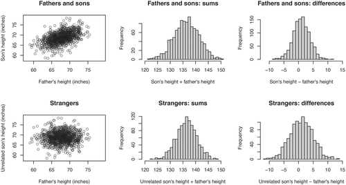
To understand the impact of correlation on the variances of sums and differences, we begin with an exercise that asks students to consider a setting where they sampled pairs of heights from two groups: fathers/sons and strangers (i.e., fathers were paired with a random unrelated son). Students are asked for which group is the variance of the sums of the paired heights larger and for which group is the variance of the differences of the paired heights larger. They are shown the scatter plots of the paired heights in Figure 1 to consider while discussing in small groups. When coming back together and discussing as a class, we view the histograms of the sums and differences of the paired heights in Figure 1. Students are able to conclude that positively correlated random variables have a larger variance of their sums and a smaller variance of their differences than independent random variables. Students typically come to this conclusion by recognizing that it is more likely to have extreme pairs where both individuals are short or both are tall when the pairs are fathers and sons. These extreme pairs result in greater variability when considering their sums and less variability when considering their differences. The heights of 1078 father–son pairs used in this example are available with data(father.son) via the UsingR R package (Verzani 2018). Note that the increased variance of sums versus differences in Figure 1 is somewhat subtle due to the moderate correlation between the heights of sons and fathers. If a more obvious contrast is desired, the sons’ heights can be simulated to be more strongly correlated with their fathers’ heights.

Fig. 1 An example to illustrate the impact of correlation on the variances of sums and differences. The pairs of heights from fathers and sons have a larger variance for their sums and a smaller variance for their differences than those from unrelated pairs.

Following this exercise, students are shown the formulas for the variance of sums and differences of random variables:$$\begin{array}{c}\text{var}(X+Y)=\text{var}(X)+\text{var}(Y)+2\times \text{cov}(X,Y)\\ \text{var}(X-Y)=\text{var}(X)+\text{var}(Y)-2\times \text{cov}(X,Y).\end{array}$$

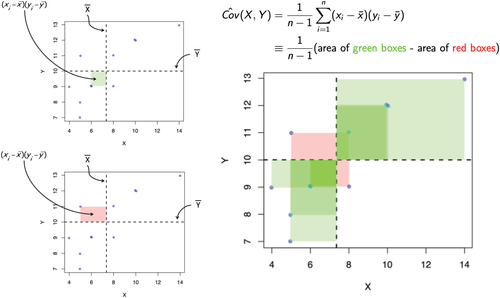
A visual representation of the definition of sample covariance is shown (Figure 2). Students see that since the father–son pairs’ heights have positive covariance, their sums of heights have a larger variance than the strangers and their differences in heights have a smaller variance than the strangers. Since independent random variables have a covariance of 0, students see that if we naively assume independence, the naive variance of sums will typically underestimate the true variance and the naive variance of differences will typically overestimate the true variance due to the positive covariance.

Fig. 2 A visual representation of the definition for sample covariance. Each data point (x_i , y_i ) has a corresponding shaded rectangle whose area is the deviation from the variables’ means, $(x_i-\overline{x})(y_i-\overline{y})$. Larger rectangles correspond to data points further from their means. Rectangles are shaded green when the variables “move together” (i.e., both values are larger or smaller than their respective means) and shaded red when they do not (e.g., one value is larger than its mean and the other is smaller). The sample covariance is the difference between the total area of the green rectangles and the red rectangles (divided by n – 1).

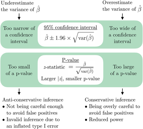
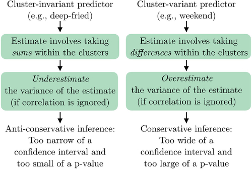
After establishing the impact of correlation on the variances of sums and differences, we connect this to the impact on inference for effects of interest involving correlated outcomes. For estimates involving sums (such as the total effect of treatment), ignoring correlation leads to an underestimated variance, which translates to too narrow of confidence intervals and too small of p-values. We call this anti-conservative (or overly liberal) inference, meaning that it is too easy to find statistically significant results even when there is no effect. This can be illustrated as “raining p < 0.05.” For estimates involving differences (such as change over time), ignoring correlation leads to an overestimated variance, which translates to too wide of confidence intervals and too large of p-values. We call this (overly) conservative inference, meaning that it is too difficult to find statistically significant results even when there is an effect. This can be illustrated as the frustrated, exasperated scientist. The impact of an underestimated or overestimated variance of an effect estimate is shown in Figure 3.

Fig. 3 A summary of how underestimating or overestimating the variance of the effect estimate $\widehat{\beta }$ due to ignoring correlated outcomes can lead to anti-conservative or conservative inference, respectively.

Students practice applying these concepts in an exercise that asks them to consider a randomized trial of a drug (vs. placebo) where each subject receives a treatment at two different time points. In Scenario A, each subject takes the same treatment at both time points and in Scenario B, each takes the placebo at one time point and the drug at the other. Students are asked: if the correlation between outcomes on the same subject is ignored when the data is analyzed to estimate the treatment effect, what goes wrong? Are the confidence intervals too wide or narrow? Are the p-values too large or small? In Scenario A, estimating the treatment effect will involve taking means (i.e., sums) of the correlated outcomes within subjects, and thus ignoring the correlation will produce confidence intervals that are too narrow and p-values that are too small. Having two observations per subject for the same intervention provides less information about the treatment effect than having twice as many independent subjects. In Scenario B, estimating the treatment effect will involve taking differences of the correlated outcomes within subjects, and thus ignoring the correlation will produce confidence intervals that are too wide and p-values that are too large. This analysis ignores that each subject is serving as their own control, which provides more information than having twice as many independent subjects.

Students with more quantitative backgrounds might derive the variance of the estimator in these two settings to directly show the impact of improperly ignoring the correlation. This derivation is included in the Appendix.

2.2 Active Learning Classroom Activity

Following the introductory lecture described above, students work on an active learning classroom activity to reinforce what was introduced in the lecture. Students work in groups and we discuss their findings as a whole class at multiple points throughout the activity. Students are not graded on the activity, but the concepts learned are tested on future weekly quizzes and applied on their graded homework. We typically reconvene as an entire class to discuss their findings at three points after most students have completed that part of the activity. We typically spend a total of 90 min on the activity, which can be split between two class periods if desired. This time is split between introducing the activity (10 min), working on and discussing Part 1 (25 min), working on and discussing Part 2 (25 min), working on and discussing Part 3 (20 min), and wrapping up the activity as a class (10 min). For each of the activity parts, about half of the time is allotted for small group work and the other half to discussion as an entire class, though this can be adapted based on the average skill level of students and how heterogeneous the skill levels are. The course tends to have a wide range of skill levels and thus spending ample time going through the questions as an entire group is worthwhile. The introduction, the three parts of the activity, and the wrap-up are discussed below.

2.2.1 Activity Introduction

Given the student backgrounds, many have not yet encountered the concept of statistical simulation and thus this must be introduced in addition to the particulars of the activity. It can be explained that it can be tricky to know whether or not a method is working appropriately in statistics. Unlike a lab experiment where the mouse dies or your solution does not precipitate, an invalid statistical analysis can look completely normal with estimates, confidence intervals, and p-values provided in the output. In statistics, we have two main approaches for showing a method “works” as intended: proof via math or by employing simulations. When given the choice between the two, the students happily agree to use simulations. With simulations, we analyze “fake” data for which we know the truth lots of times.

We discuss what it means for a method to “work” properly in terms of the estimate, confidence interval, and p-value. For the estimate, we like it to be unbiased, meaning that the average of the estimates across the simulations is equal to the true value. For the 95% confidence interval, we want it to have the appropriate coverage, meaning that it captures the true value 95% of the time. For the p-value, we want the Type I error, or proportion of statistically significant p-values under the null, to be equal to the α level (e.g., 0.05). When considering the alternative (i.e., when there is an effect), the proportion of statistically significant p-values is called power. We want to choose a method that has the highest power given that it follows the rules (i.e., unbiased, correct coverage, correct Type I error rate). (While there are instances where biased estimators (e.g., lasso) are preferable [Hastie et al. 2009], this is generally beyond the scope of this course.)

After introducing the idea of simulation studies and the metrics used to judge a method’s performance, we discuss the study background. We are interested in which factors are associated with daily food booth sales at the Minnesota State Fair. To this end, we collect data from 50 food booths for six different days during the fair. We want to see whether there is evidence of an association between daily food booth sales and (a) whether it is a weekend and (b) whether the booth sells deep-fried food. In this alternate reality, we are able to run this study many, many times, and we consider the analysis results across the repeated runs of the study under different scenarios to see the impact of ignoring correlated outcomes. In particular, we repeat the study 1000 times each under four different scenarios: (a) There is no effect of selling deep-fried food on booth sales, (b) There is an effect of selling deep-fried food on booth sales, (c) There is no effect of the weekend on booth sales, and (d) There is an effect of the weekend on booth sales.

Throughout the activity students become more proficient in the terminology that is used to judge the performance of statistical methodology. Having students learn some technical terminology is a necessity in a correlated data course as understanding the properties of the estimators becomes crucial in appreciating the differences between different methods. For example, later in the course, we further introduce the concepts of consistency and efficiency to understand the consequences of choosing different working correlations in a GEE model. Having some exposure to the concept of the sampling distribution and the performance of estimators across repeated sampling is helpful when introducing these new technical concepts. Consistency can be introduced as the asymptotic extension of unbiasedness and efficiency builds upon the students’ understanding of coverage.

2.2.2 Activity Part 1: Background and Making Predictions

After introducing the activity, students work in small groups to complete the first part of the activity. The first four questions help to orient the students to the study setting:

1. What is the study design? An observational, longitudinal study

2. What is the outcome of interest? Daily booth sales

3. What are the predictors of interest? Whether a booth sells deep-fried food and whether it is the weekend

4. What is the source of correlation in the outcomes? Multiple measurements (on different days) were taken for each booth

The next two questions review the terminology used to assess the performance of statistical methods:

1. When you have conservative inference, what is the consequence on the p-values and confidence intervals? How about for anti-conservative inference? Conservative inference means that the confidence intervals are too wide (i.e., coverage probability $>95\%$) and the p-values are too large (i.e., Type I error rate $<5\%$). Anti-conservative inference means that the confidence intervals are too narrow (i.e., coverage probability $<95\%$) and the p-values are too small (i.e., Type I error rate $>5\%$).

2. What should the Type I error rate and a confidence interval’s coverage probability be? Assuming a (typical) alpha level of 0.05, the Type I error rate should be 5% and the coverage probability should be 95%.

The final question for this part asks students to predict the results of the simulation. In particular, it specifies that the following linear regression model is fit:$$E\left[\text{BoothSales}\right]={\beta }_0+{\beta }_1\times \text{Weekend}+{\beta }_2\times \text{DeepFried},$$which treats all of the 300 (50 booths × 6 days) outcomes as independent. Students are asked to predict:

1. When there is truly an effect, will you have correct, conservative, or anti-conservative inference when estimating the effect on booth sales of (1) the weekend and (2) selling deep-fried food?

When discussing this part as an entire class, you can poll students on their predictions for the two predictors, which they can later compare to their findings after the activity.

2.2.3 Activity Part 2: First Half of the Results Interpretation

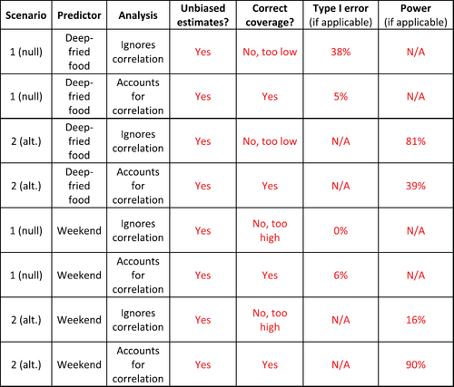
At the end of the discussion for Part 1 of the activity, students are walked through the results output to orient them. There are a total of eight sets of results (= two scenarios [under the null or alternative] × two predictors [deep-fried food or weekend] × two analysis approaches [ignoring correlation or accounting for it]). An example of the results for one of the eight sets of results is shown in Figure 4. Students then work in their small groups to interpret the results for the settings corresponding to the deep-fried food predictor and complete the top half of their results table (Figure 5). In addition, they answer a question that asks them to summarize the impact of ignoring correlation in their analysis when estimating the effect of deep-fried food on booth sales. From the results, they see that even when ignoring correlation, the estimates of the effect of deep-fried food on booth sales are unbiased. However, the Type I error rate is greatly inflated (38% instead of 5%) due to greatly underestimating the variance of the estimate. This leads to confidence intervals that are too narrow and only capture the true value 62% of the time, instead of 95%, which is called anti-conservative inference. The underestimation of the variance comes from the positive correlation of outcomes within the same food booth. The predictor of deep-fried food is constant within clusters (food booths), so estimating its effect involves taking sums of the correlated outcomes within booths.

Fig. 4 Example results, corresponding to the results for the deep-fried food predictor under the null hypothesis when using an analysis approach that ignores correlation, for one of the eight settings that students investigate. The plots summarize the results from the analyses of the 1000 studies run for this setting. The left plot is a histogram of the 1000 point estimates ($\widehat{\beta }$’s), the middle plot shows 50 of the 1000 confidence intervals where the blue line indicates the truth, and the left plot shows a histogram of the 1000 p-values obtained.

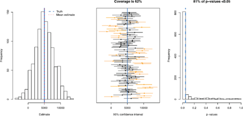
Fig. 5 Results table for the activity with the solutions that students complete shown in red.

2.2.4 Activity Part 3: Second Half of the Results Interpretation

After discussing the first half of the results table (Figure 5) as a class, students complete the second half of the results table and summarize the impact of ignoring correlation in their analysis when estimating the effect of the weekend on booth sales. From the results, they can once again see that even when ignoring correlation, the estimates of the effect of the weekend on booth sales are unbiased. However, the Type I error rate is tiny (it’s 0%!) due to overestimating the variance of the estimate. This leads to confidence intervals that are too wide such that they capture the true value 100% of the time, instead of 95%, which we call conservative inference. The overestimation of the variance comes from the fact that there is positive correlation of outcomes within the same food booth and the predictor of weekend varies within clusters (food booths). Estimating its effect involves taking differences of the correlated outcomes within booths.

There are two additional wrap-up questions to help students apply what they have learned. The first question asks them to agree or disagree with a collaborator’s suggestion to ignore correlation since the likelihood of obtaining a statistically significant result is much higher when estimating the effect of selling deep-fried food. Students should object to this collaborator’s suggestion, since the analysis ignoring correlation is invalid, which can be seen from the inflated Type I error rate under the null. Even when there is no effect, the null hypothesis is rejected 38% of the time making the results from the analysis ignoring correlation untrustworthy. The second wrap-up question asks students to apply what they’ve learned to predict the impact on inference if they use a statistical approach ignoring the correlated outcomes for two new predictors: the weather (sunny vs. rainy) and first-time booth status. When estimating the effect of weather and ignoring correlation, students should conclude that there will be conservative inference, since the predictor of weather will vary within clusters. (This is analogous to the weekend predictor.) When estimating the effect of being a first-time booth and ignoring correlation, students should predict anti-conservative inference, since the predictor of being a first-time booth is constant within clusters. (This is analogous to the deep-fried food predictor.)

2.2.5 Activity Wrap-Up

After finishing the activity, it is reemphasized how the findings from the activity connect to what students learned in the introductory lecture. We first write out the structure of the state fair dataset for a single replication to further emphasize the two types of predictors: those that do not vary within cluster (e.g., deep-fried food) and those that do vary within cluster (e.g., weekend). An example of this is in Figure 6. We then make a flowchart on a whiteboard to illustrate the reasoning that helps us to conclude that, when ignoring correlation, the resulting inference will be anti-conservative for cluster-invariant predictors and conservative for cluster-variant predictors. A formal version of this flowchart is in Figure 7, though drawing this on the whiteboard step by step may be the most helpful to students.

Fig. 6 Example dataset for a single replicate in “long” form with a single observation per row and the observations from a single cluster spanning multiple rows.

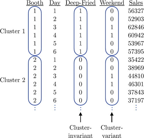
Fig. 7 A flowchart summarizing the implications of ignoring correlation between outcomes for predictors that vary or do not vary within cluster. For intuition about the second connection, have students recall the example about the variability of the sums and differences of father–son heights. For more detail about the third connection, see Figure 3.

3 Integrating Intuition Throughout the Course

In this section, it is described how the students’ intuition about the impact of ignoring correlation between outcomes can be further reinforced during later course activities and how their intuition can be used to motivate extensions of standard sample size and power calculations to the correlated data setting. Lastly, the issue of predictors that vary both between and within clusters is addressed.

3.1 Comparing Results from Correlated Data Methods to Naive Methods

After initially introducing the impact of ignoring correlation when analyzing correlated outcomes, the intuition is repeatedly emphasized throughout the course. In particular, when introducing new methods (e.g., GLMM and GEE), the model results for the new method are presented alongside the model results from the “naive” method, which ignores the correlation between outcomes. Table 1 shows an example of this. Students are able to see that the point estimates (i.e., $\widehat{\beta }$’s) remain exactly the same or very similar, but the standard errors for the point estimates change in a predictable way depending on whether the predictor is cluster-variant or cluster-invariant. The naive GLM standard errors are larger for within-cluster effects (${\widehat{\beta }}_1$ in Table 1) and smaller for between-cluster effects (${\widehat{\beta }}_2$). When presenting the naive results to students, it is very important to stress that the GLM should not be used to analyze correlated data and that the reason for fitting the GLM is to help illustrate the differences between the results from a GLM versus those from an appropriate analysis using GEE or GLMM. It is also important to emphasize that many decimal places are shown for comparison purposes. In practice, students should report fewer digits.

Table 1 Comparison of the point estimates and standard errors (SEs) obtained for a correlated dataset using Gaussian generalized estimating equations (GEE) models with different working correlations and a naive linear regression model that assumes independent outcomes.

	${\widehat{\beta }}_0$ (SE)	${\widehat{\beta }}_1$ (SE)	${\widehat{\beta }}_2$ (SE)
GEE
(independence)	0.15328 (0.01323)	−0.00770 (0.00251)	−0.02980 (0.01300)
GEE
(exchangeable)	0.15328 (0.01323)	−0.00770 (0.00251)	−0.02980 (0.01300)
GEE (AR-1)	0.15628 (0.01364)	−0.00824 (0.00258)	−0.03083 (0.01289)
GEE
(unstructured)	0.15439 (0.01333)	−0.00754 (0.00252)	−0.03133 (0.01271)
Naive model	0.15328 (0.01123)	−0.00770 (0.00298)	−0.02980 (0.00867)

NOTE: The naive model overestimated the SE for ${\widehat{\beta }}_1$ since the corresponding covariate varied within clusters and underestimated the SE for ${\widehat{\beta }}_2$ since the corresponding covariate varied between clusters. Note that for this particular analysis, the data were balanced (i.e., the same number of observations per cluster) and complete (i.e., no missing data), thus, the results using an independence and exchangeable working correlation were exactly the same.

Students repeatedly practice noticing these patterns through homework assignments and evaluative quizzes and tests. On homework assignments analyzing correlated outcomes, students are sometimes asked to also fit a “naive” method like linear regression to observe the impact on the point estimates and standard errors. Similarly, students are asked on quizzes and tests to postulate how the model results from fitting a correlated data method would change if the correlation was erroneously ignored and a standard method assuming independent outcomes was used instead. Examples of these questions are shown in Table 2.

Table 2 Example questions and answers used in homework assignments, quizzes, and tests throughout the semester to reinforce students’ intuition about the impact of ignoring correlation between outcomes.

Sample questions	Sample answers
True or False: After analyzing longitudinal data using a GEE model, you find out that there are several pairs of siblings in your study, which examines an outcome thought to be impacted by genetic factors. Your original GEE results will still provide trustworthy inference since GEE uses sandwich variances that help when the variance structure is incorrectly specified.	False. GEE requires independent clusters (which would be violated by having siblings in your study) to obtain trustworthy inference.
Your collaborator fits a GLM model to this data and finds that the confidence interval for the intervention effect is narrower than the one you obtained using the GEE model. Seeing this, he insists that his analysis is preferable. In one to two sentences, provide a response to him.	The GLM model is inappropriate as it assumes independent outcomes. When our analysis ignores correlated outcomes, we will obtain too narrow of confidence intervals for cluster-invariant predictors (like intervention in this case), which results in an inflated Type I error rate.
How do the standard errors for the coefficients in your GLM model compare to the standard errors in the GEE models? Explain how this fits with what we have learned previously about the impact of ignoring correlated outcomes in analyses.	The standard errors for the variables that do not vary within cluster (i.e., intercept, treatment) are smaller in the GLM than the GEE models. In contrast, the standard errors for the variables that do vary within cluster (i.e., time, time by treatment interaction) are larger in the GLM than the GEE models. This fits with what we have learned: ignoring correlation will lead to overly narrow confidence intervals for between-cluster effects and overly wide confidence intervals for within-cluster effects.
Your collaborator performs a crossover study in which each subject receives the experimental treatment at one time point and the placebo at the other time point. He compares the outcomes between the experimental treatment and placebo using a two-sample t-test. The obtained p-value will be too _________ and the confidence interval will be too _________, which we call inference.	large / wide / conservative
True or False: Analyzing correlated outcomes as if they are independent always leads to obtaining too small of p-values.	False. Ignoring correlation can lead to too small or too large of p-values, depending on whether the covariate is cluster-invariant or cluster-variant.

3.2 Sample Size and Power Calculations for Correlated Outcomes

Sample size and power calculations are one of the special topics discussed at the end of the course. Given the foundation built during the rest of the course, students are well positioned to understand how standard sample size and power calculations can be modified to account for correlated outcomes. In the course, we discuss simple extensions of standard calculations using the concept of effective sample size, the number of independent observations needed to yield the same amount of information that the correlated observations provide. For example, we consider how the required sample size can be modified for between-cluster and within-cluster predictors by assuming the same number of observations n in each of the K clusters, equal variability of the outcomes in each cluster, and equal correlation ρ of observations within the same cluster. The effective sample size is equal to the total number of correlated observations (n × K) divided by the design effect. For between-cluster predictors, the design effect is $1+(n-1)\times \rho$, thus, requiring more observations than if using a study design with independent outcomes. For within-cluster predictors, the design effect is $1-\rho$, which reduces the required sample size relative to all independent outcomes (Vittinghoff et al. 2012). Students learn that when planning studies, the sample size and power calculations for studies with correlated data must take into account the correlation structure and the type of effect of interest (within-cluster vs. between-cluster).

3.3 Predictors that Vary Between and Within Clusters

Within-cluster predictors are those whose values vary within cluster but have the same average across clusters. Though we have not yet discussed the latter point, all of the within-cluster predictors considered thus, far meet these criteria, since each cluster has the same values of the predictor and thus the cluster-level means of the predictors are all equal. This is often the case in designed experiments with no missing data (e.g., the predictor of time where each subject is measured at the same post-intervention time points). However, there are many instances in which a predictor may vary both between and within clusters. For example, in a study of the impact of hormone levels, the women’s hormone levels will fluctuate over time and the average hormone levels will vary between women. These between- and within-cluster effects can be isolated by including two versions of the predictor in the mean model: (a) a between-cluster effect equal to the cluster-level mean of the predictor and (b) a within-cluster effect equal to the cluster-centered predictor (e.g., see sec. 7.7.2 of Vittinghoff et al. 2012). This concept may be best introduced later in the course when students are more comfortable with the concepts related to correlated data. However, it is recommended to use examples in this activity that involve predictors that purely vary between clusters or within clusters.

4 Modifications and Extensions

In this section, potential modifications and extensions of the activity to different course settings are described.

The data context can easily be adapted to be relevant to the students in your course. This activity was developed for a University of Minnesota course taught every fall that begins on the day after the conclusion of the Minnesota State Fair. While using simulated data is necessary, the simulated data should be plausible with a real-world context that students easily understand. This realistic simulated data can be based on an actual dataset that students will analyze later in the course. In modifying the data context, the basic components to choose are the clusters (e.g., food booths), outcome (e.g., daily food booth sales), cluster-variant predictor (e.g., weekend vs. not), and cluster-invariant predictor (e.g., deep-fried food vs. not).

The students’ coding skill levels are very heterogeneous. Instruction is offered in both SAS and R, and students can choose which they use. Given these factors, it has worked well to provide the simulation results to the students, rather than having them produce the results themselves. However, in a more advanced course or with less variation in coding skill levels, it may be instructive to have students produce the results plots themselves. Given that this activity precedes students learning about correlated data methods, a “black box” regression function for the correlated data method (e.g., linear mixed effect model) could be provided or the results from applying the correlated data method could be directly provided with students producing the results for applying standard regression techniques that do not account for correlated outcomes. If students are expected to produce the results themselves, significantly more time would be needed to complete the activity and thus the instructor could consider adapting this into a homework assignment or multiple class periods in a flipped classroom setting. Regardless, the instructor should ensure that the coding aspect of the assignment does not obscure the main learning objective of developing a conceptual understanding of the impact of ignoring correlation between outcomes.

A compromise between providing the simulation results directly or having students produce the simulation results themselves is that an applet could be developed using Shiny (Chang et al. 2021) to provide more flexibility. For example, in a more advanced course, the applet could allow students to vary the within-cluster correlation and observe the impact on the results.

A possible extension of this activity could be to revisit the activity later in the semester to demonstrate the impact of the choice of working correlation structure in GEE on efficiency. For example, instead of comparing a method that accounts for correlated outcomes versus not, as in the original activity, the results from GEE models with different working correlations could be compared to demonstrate the impact of choosing the “correct” working correlation versus an alternative one. Students would be able to see that while all reasonable choices for working correlation provide confidence intervals with the correct coverage, the confidence intervals are, on average, narrower when the “correct” working correlation is chosen.

5 Conclusion

Analyzing correlated outcomes in an appropriate manner is a key competency in data analysis. However, intuition about the exact consequences of ignoring correlation by applying standard regression techniques does not come easily for many students. Thus, we discussed an in-class activity that can be used to develop students’ intuition at the beginning of a course on statistical methods for correlated data.

This activity has been used twice previously in classes of 49 and 51 students. During the first iteration, the activity was used as part of an in-person course. Students worked on the activity in small groups self-selected by the students. During the second iteration, the course was taught fully online in a synchronous fashion due to the COVID-19 pandemic. Students worked together in Zoom breakout rooms via instructor-assigned random groups of four to five students. In both instances, the instructor was available for questions throughout the activity and would reconvene the entire class at multiple points to discuss their findings. During the second iteration, individual student polling was used to have students share their predictions and conclusions. Prior to reviewing the simulation results, 56% (28/50) of students correctly identified that the cluster-variant predictor of the weekend would result in conservative inference, and 82% (41/50) of students correctly identified that the cluster-invariant predictor of deep-fried food would result in anti-conservative inference. There was significant improvement following the activity when students were asked to generalize their findings to a new set of predictors. For these new predictors, 78% (39/50) of students correctly identified that the cluster-variant predictor would result in conservative inference, and 98% (49/50) of students correctly identified that the cluster-invariant predictor would result in anti-conservative inference.

In addition to improving student comprehension, several students identified the in-class activities (the activity described here being the first of three in the course) as being helpful for comprehension in free-response answers to the question “What were the strengths of this course?” on an anonymous end-of-semester student evaluation of teaching. One student commented, “Sometimes the concepts we cover can be a bit abstract and these in-class exercises provide clarification and intuitive understanding.” Another student shared, “I like the activities we do together that help concretize the concepts.” The in-class format was found to be useful: “The activities in class are really helpful. Lectures on stats can only get me so far—I need to interact with the material, ideally in a “supported” way (i.e., in class, with immediate feedback) to feel like I’m really learning the concepts.” Another noted, “The use of in class exercises and worksheets made the class much more interactive, which greatly facilitated my learning.” All comments relating to the in-class activities were positive, such as, “The activities are helpful—I typically learn a lot from working through the projects.”

This activity is useful as it allows students to uncover what goes wrong when correlated data is analyzed inappropriately and motivates the need for the methods taught in the course. Students become more comfortable with the technical language needed to understand the advantages and disadvantages of different correlated data approaches. Further, students work in small groups during the first week of class, helping to create a communal, collaborative classroom environment.

Acknowledgments

I thank the editor, associate editor, and three anonymous reviewers for their useful suggestions that improved the clarity and content of this work.

Supplementary Materials

Activity printout: A ready-to-use version of the activity with a questions sheet and results sheet. (Both available as PDF files and Word documents)

Activity solutions: Example solutions for the activity. (PDF file and Word document).

Simulation code: R code to reproduce the simulation results presented in the activity. (R script)

Appendix

We derive the variance of the ordinary least squares (OLS) estimator in the two correlated data settings discussed in the example in Section 2.1. This example considers a randomized trial of a drug (vs. placebo) where each subject receives a treatment at two different time points. In Scenario A, each subject takes the same treatment at both time points and in Scenario B, each takes the placebo at one time point and the drug at the other. We denote the response vector for the K participants as $\mathbf{Y}={(Y_{11},Y_{12},Y_{21},Y_{22},\dots ,Y_{K1},Y_{K2})}^T$. We are interested in estimating the treatment effect using the mean model ${\beta }_0+{\beta }_1\times (\text{Treatment})=\mathbf{X}\mathbf{\beta }$ where $\mathbf{\beta }={({\beta }_0,{\beta }_1)}^T$ and ${\mathbf{X}}_{\mathbf{A}}={\left[\begin{array}{ccccc}1& \cdots 1& 1& \cdots & 1\\ 1& \cdots 1& 0& \cdots & 0\end{array}\right]}^T$ in Scenario A and ${\mathbf{X}}_{\mathbf{B}}={\left[\begin{array}{cccccc}1& 1& 1& 1& \cdots 1& 1\\ 1& 0& 1& 0& \cdots 1& 0\end{array}\right]}^T$ in Scenario B. We assume that there is equal variance ${\sigma }^2$ across subjects, the within-subject observations have correlation equal to ρ, and the between-subject observations are uncorrelated. Thus, the $\text{var}(\mathbf{Y})={\sigma }^2\left[\begin{array}{ccccc}1& \rho & \cdots & & 0\\ \rho & 1& & & \\ ⋮& & \ddots & & ⋮\\ & & & 1& \rho \\ 0& & \cdots & \rho & 1\end{array}\right]$. We now derive the true variance of the OLS estimator, $\widehat{\mathit{\beta }}={({\mathbf{X}}^T\mathbf{X})}^{-1}{\mathbf{X}}^T\mathbf{Y}$, under Scenarios A and B.

In Scenario A,$$\begin{array}{l}\text{var}(\widehat{\beta })={(X_A^T{X}_A)}^{-1}{X}_A^T\text{var}(Y)X_A{(X_A^T{X}_A)}^{-1}\\ =\frac{{\sigma }^2}{K^2}\left[\begin{array}{cc}1& -1\\ -1& 2\end{array}\right]\left[\begin{array}{ccccc}1& \cdots 1& 1& \cdots & 1\\ 1& \cdots 1& 0& \cdots & 0\end{array}\right]\left[\begin{array}{ccccc}1& \rho & \cdots & & 0\\ \rho & 1& & & \\ ⋮& & \ddots & & ⋮\\ & & & 1& \rho \\ 0& & \cdots & \rho & 1\end{array}\right]\\ {\left[\begin{array}{ccccc}1& \cdots 1& 1& \cdots & 1\\ 1& \cdots 1& 0& \cdots & 0\end{array}\right]}^T\left[\begin{array}{cc}1& -1\\ -1& 2\end{array}\right]\\ =\frac{{\sigma }^2}{K}\left[\begin{array}{cc}1+\rho & -1-\rho \\ -1-\rho & 2(1+\rho )\end{array}\right]\end{array}$$so the true variability of the treatment effect in Scenario A is $\text{var}({\widehat{\beta }}_1)=\frac{2{\sigma }^2(1+\rho )}{K}$. Therefore, using the naive variance of $\frac{2{\sigma }^2}{K}$ will lead to underestimating the variance of the treatment effect in settings where the observations within individuals are positively correlated ($\rho >0$).

Similarly, in Scenario B,$$\begin{array}{c}\text{var}(\widehat{\mathit{\beta }})={({\mathbf{X}}_{\mathbf{B}}^T{\mathbf{X}}_{\mathbf{B}})}^{-1}{\mathbf{X}}_{\mathbf{B}}^T\text{var}(\mathbf{Y}){\mathbf{X}}_{\mathbf{B}}{({\mathbf{X}}_{\mathbf{B}}^T{\mathbf{X}}_{\mathbf{B}})}^{-1}\\ =\frac{{\sigma }^2}{K^2}\left[\begin{array}{cc}1& -1\\ -1& 2\end{array}\right]\left[\begin{array}{cccccc}1& 1& 1& 1& \cdots 1& 1\\ 1& 0& 1& 0& \cdots 1& 0\end{array}\right]\left[\begin{array}{ccccc}1& \rho & \cdots & & 0\\ \rho & 1& & & \\ ⋮& & \ddots & & ⋮\\ & & & 1& \rho \\ 0& & \cdots & \rho & 1\end{array}\right]\\ \mathrm{\hspace{1em}}\mathrm{\hspace{1em}}{\left[\begin{array}{cccccc}1& 1& 1& 1& \cdots 1& 1\\ 1& 0& 1& 0& \cdots 1& 0\end{array}\right]}^T\left[\begin{array}{cc}1& -1\\ -1& 2\end{array}\right]\\ =\frac{{\sigma }^2}{K}\left[\begin{array}{cc}1& \rho -1\\ \rho -1& 2(1-\rho )\end{array}\right]\end{array}$$so the true variability of the treatment effect in Scenario B is $\text{var}({\widehat{\beta }}_1)=\frac{2{\sigma }^2(1-\rho )}{K}$. Therefore, using the naive variance of $\frac{2{\sigma }^2}{K}$ will lead to overestimating the variance of the treatment effect in settings where the observations within individuals are positively correlated ($\rho >0$).

References

- Ananth, C. V., Platt, R. W., and Savitz, D. A. (2005), “Regression Models for Clustered Binary Responses: Implications of Ignoring the Intracluster Correlation in an Analysis of Perinatal Mortality in Twin Gestations,” Annals of Epidemiology, 15, 293–301. DOI: https://doi.org/10.1016/j.annepidem.2004.08.007.
- Bates, D., Mächler, M., Bolker, B., and Walker, S. (2015), “Fitting Linear Mixed-Effects Models Using lme4,” Journal of Statistical Software, 67, 1–48. DOI: https://doi.org/10.18637/jss.v067.i01.
- Cannon, M. J., Warner, L., Taddei, J. A., and Kleinbaum, D. G. (2001), “What can go Wrong When you Assume that Correlated Data are Independent: An Illustration from the Evaluation of a Childhood Health Intervention in Brazil,” Statistics in Medicine, 20, 1461–1467. DOI: https://doi.org/10.1002/sim.682.
- Carver, R., Everson, M., Gabrosek, J., Horton, N., Lock, R., Mocko, M., Rossman, A., Rowell, G. H., Velleman, P., Witmer, J., and Wood, B. (2016), “Guidelines for Assessment and Instruction in Statistics Education (GAISE) College Report 2016,” Available at https://www.amstat.org/asa/files/pdfs/GAISE/GaiseCollege_Full.pdf.
- Chang, W., Cheng, J., Allaire, J., Sievert, C., Schloerke, B., Xie, Y., Allen, J., McPherson, J., Dipert, A., and Borges, B. (2021), shiny: Web Application Framework for R. R package version 1.7.0.
- Du Toit, G., Roberts, G., Sayre, P. H., Bahnson, H. T., Radulovic, S., Santos, A. F., Brough, H. A., Phippard, D., Basting, M., Feeney, M., Turcanu, V., Sever, M. L., Lorenzo, M. G., Plaut, M., Lack, G., and The LEAP Study Team. (2015), “Randomized Trial of Peanut Consumption in Infants at Risk for Peanut Allergy,” The New England Journal of Medicine, 372, 803–813. DOI: https://doi.org/10.1056/NEJMoa1414850.
- Fitzmaurice, G. M., Laird, N. M., and Ware, J. H. (2012), Applied Longitudinal Analysis, Hoboken, NJ: Wiley.
- Halekoh, U., Højsgaard, S., and Yan, J. (2006), “The R package geepack for Generalized Estimating Equations,” Journal of Statistical Software, 15, 1–11. DOI: https://doi.org/10.18637/jss.v015.i02.
- Hastie, T., Tibshirani, R., Friedman, J. H., and Friedman, J. H. (2009), The Elements of Statistical Learning: Data Mining, Inference, and Prediction (Vol. 2), New York: Springer.
- Henao-Restrepo, A. M., Longini, I. M., Egger, M., Dean, N. E., Edmunds, W. J., Camacho, A., Carroll, M. W., Doumbia, M., Draguez, B., Duraffour, S., Enwere, G., Grais, R., Gunther, S., Hossmann, S., Konde, M. K., Kone, S., Kuisma, E., Levine, M. M., Mandal, S., Norheim, G., Riveros, X., Soumah, A., Trelle, S., Vicari, A. S., Watson, C. H., Keita, S., Kieny, M. P., and Rottingen, J.-A. (2015), “Efficacy and Effectiveness of an rVSV-vectored Vaccine Expressing Ebola Surface Glycoprotein: Interim Results from the Guinea Ring Vaccination Cluster-Randomised Trial,” The Lancet, 386, 857–866. DOI: https://doi.org/10.1016/S0140-6736(15)61117-5.
- Howie, E. K., Beets, M. W., and Pate, R. R. (2014), “Acute Classroom Exercise Breaks Improve On-task Behavior in 4th and 5th Grade Students: A Dose–Response,” Mental Health and Physical Activity, 7, 65–71. DOI: https://doi.org/10.1016/j.mhpa.2014.05.002.
- Laird, N. M., and Ware, J. H. (1982), “Random-Effects Models for Longitudinal Data,” Biometrics, 38, 963–974. DOI: https://doi.org/10.2307/2529876.
- Liang, K.-Y., and Zeger, S. L. (1986), “Longitudinal Data Analysis Using Generalized Linear Models,” Biometrika, 73, 13–22. DOI: https://doi.org/10.1093/biomet/73.1.13.
- Lyman, F. T. (1981), “The Responsive Classroom Discussion: The Inclusion of all Students,” in Mainstreaming Digest: A Collection of Faculty and Student Papers, ed. A. S. Anderson, pp. 109–113. College Park, MD: University of Maryland.
- Sainani, K. (2010), “The Importance of Accounting for Correlated Observations,” PM&R, 2, 858–861.
- Schneiter, K., and Symanzik, J. (2013), “An Applet for the Investigation of Simpson’s Paradox,” Journal of Statistics Education, 21, 1–20.
- Vaughan, T. S., and Berry, K. E. (2005), “Using Monte Carlo Techniques to Demonstrate the Meaning and Implications of Multicollinearity,” Journal of Statistics Education, 13, 1–9.
- Verzani, J. (2018), UsingR: Data Sets, Etc. for the Text “Using R for Introductory Statistics,” (2nd ed.), R package version 2.0-6.
- Vittinghoff, E., Glidden, D. V., Shiboski, S. C., and McCulloch, C. E. (2012), Regression Methods in Biostatistics: Linear, Logistic, Survival, and Repeated Measures Models, New York: Springer-Verlag.
- Wang, X., Reich, N. G., and Horton, N. J. (2019), “Enriching Students’ Conceptual Understanding of Confidence Intervals: An Interactive Trivia-based Classroom Activity,” The American Statistician, 73, 50–55. DOI: https://doi.org/10.1080/00031305.2017.1305294.
- Zeger, S. L., and Liang, K.-Y. (1986), “Longitudinal Data Analysis for Discrete and Continuous Outcomes,” Biometrics, 42, 121–130. DOI: https://doi.org/10.2307/2531248.