
 ?Mathematical formulae have been encoded as MathML and are displayed in this HTML version using MathJax in order to improve their display. Uncheck the box to turn MathJax off. This feature requires Javascript. Click on a formula to zoom.
ABSTRACT
In this article, we have suggested a class of estimators for the estimation of the population variance of the variable of interest. The proposed estimators used some certain known information of the auxiliary variable, such as kurtosis, coefficient of variation, and the minimum and maximum values. The properties of the suggested class of estimators such as the bias and mean squared error (MSE) are obtained up to the first order of approximation. In order to check the performances of the estimators and to verify the theoretical results, we conducted a simulation study. The results of the simulation study show that the proposed class of estimators have lower MSE than other existing estimators. This holds for all simulation scenarios. In the application part, we used data from Statistical Bureau of Pakistan, and from the Textbook of Cochran, which also confirms that the suggested class of estimators is more efficient than the usual unbiased variance estimator, ratio estimator, traditional regression estimator, and other existing estimators in survey literature.
1. Introduction
The purpose of survey sampling is to get accurate information about the characteristics of the population for improving the efficiency of the estimators under study at the lowest costs, less time and human efforts (for more details, see Yang et al. (Citation2020)). In several populations, there has been a few extreme values and to estimate the unknown population parameters without including this information is very sensitive. In which case, the results will be underestimated or overestimated. To solve this issue, it is important to use this information in estimating the population parameters. Isaki (Citation1983), Bahl and Tuteja (Citation1991), Upadhyaya and Singh (Citation1999), Kadilar and Cingi (Citation2006), Dubey and Sharma (Citation2008), H. Singh and Chandra (Citation2008), Shabbir and Gupta (Citation2010), H. P. Singh and Solanki (Citation2013), and Yadav et al. (Citation2015) have all suggested some wider classes of estimators for estimating finite population variance. Consider a finite population of size
units. Let
and
be the values of the study variable
and the auxiliary variable
for the
units respectively. Let
and
be the population mean of the study and the auxiliary variable, respectively. It is further assumed that
and
be the population variances of the study as well as auxiliary variable, respectively.
To estimate the unknown population parameter , we select a random sample of size
units from the population by using simple random sampling without replacement (SRSWOR). Let
and
be the sample means of the study and the auxiliary variables, respectively, and their corresponding sample variances are
and
, respectively.
To find the bias and MSE for different estimators, we define the following terms. Let ,
and
such that
for i = 0, 1, 2.
where ,
,
,
. Also
, where
. Here
and
are the population coefficients of kurtosis.
The usual variance estimator of [1] for population variance is given by
Isaki (Citation1983) suggested a ratio-type estimator for the variance of the study variable , which is denoted by
[2], and is given by
Expressions for bias and MSE of , in sample random sampling (SRS) are given by
and
The classical regression estimator [3] in SRS is given by
where is the sample regression coefficient. The MSE of the estimator
, is given by
where
Bahl and Tuteja (Citation1991) suggested an exponential ratio-type estimator for the population variance of the study variable , which is denoted by
[4] and is given by:
Expressions for bias and MSE respectively of , are given by
and
Upadhyaya and Singh (Citation1999) proposed a ratio-type estimator [5], that uses the kurtosis of an auxiliary variable in SRS, given by
Expressions for bias and MSE respectively of , are given by
and
where
Kadilar and Cingi (Citation2006) suggested a class of ratio estimators [6–8] which are given by
where is the population coefficient of variation.
Expressions for bias and MSE’s respectively of , in SRS are given by
and
where
2. Proposed estimators
Motivated by Daraz et al. (Citation2018), we proposed an improved class of estimators for estimating the finite population variance using certain known population parameters under simple random sampling scheme. The proposed estimator is given by
where and
are the unknown constants whose values are to be determined such that the MSE’s are minimum,
and
are the parameters of the auxiliary variables. Also,
and
are the scalar quantities which contain the values (0, −1, 1) from (2.1) we can generate the different classes of proposed estimator which are given in .
Table 1. Some classes of the proposed estimator
where
Properties of the proposed estimator
Rewriting (2.1) in term of errors, we have
where
By using Taylor series up to the first order of approximation, we have
Using (2.3), the bias of , is given by
where , and
. By squaring and taking expectation on both sides of EquationEquation (2.3)
(2.3)
(2.3) , we get the mean squared error by using the first order of approximation, which is given by
where
, and
.
The optimum values of and
obtained by minimizing (2.5) are
, and
. By substituting the optimum values of
and
in (2.5), we get the minimum MSE of
, which is given below:
3. Mathematical comparison
In this section, we compare the suggested class of estimator with the existing estimators
, and
.
Condition (i): By (1.1) and (2.6), if
Condition (ii): By (1.4) and (2.6), if
Condition (iii): By (1.6) and (2.6), if
Condition (iv): By (1.9) and (2.6), if
Condition (v): By (1.12) and (2.6), if
Condition (vi): By (1.17) and (2.6), if
4. Simulation study
In order to verify the theoretical results in Section 3, we have conducted a simulation study by using the idea from Agarwal et al. (Citation2012). We generated six different artificial populations of the auxiliary variable by using the following probability distributions.
• and
, •
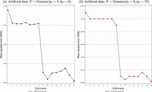
and
,
• and
.
After that, the study variable is computed as
, taking
, where
is the correlation coefficient between the study and the auxiliary variables and
is the error term.
We considered the following steps in R-Software to obtain the MSE’s of the proposed class of estimators:
Step 1: In the first step, we generated a population of size 1000 using a certain type of probability distributions.
Step 2: We obtained population total, minimum and maximum values of the auxiliary variable from Step 1. We also computed the optimum values of the unknown constants of the proposed estimator.
Step 3: We considered different sample sizes for each population to generate the samples using SRSWOR.
Step 4: For each sample size, the values of bias’s and MSE’s are computed for all the estimators considered in this paper.
Step 5: The process in Step 3 and Step 4 is repeated 50,000 times and the results for artificial populations are reported in , whereas the results of the real data sets are summarized in .
Table 2. Mean squared error (MSE) of the estimators using the artificial populations
Table 3. Mean squared error (MSE) of the estimators using empirical data sets
Finally, the MSE’s of the estimators over all replications are obtained by using the following formula. , for
.
Figure 1. Graphical display of the MSE’s results of the estimators using the artificial data
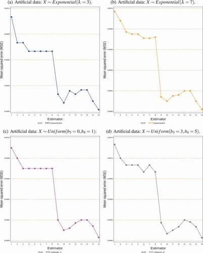
Figure 2. Graphical display of the MSE’s results of the estimators using the artificial data
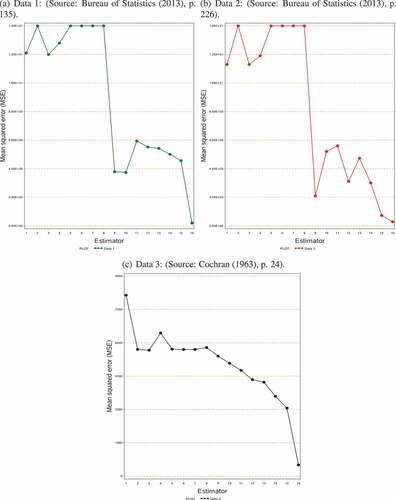
5. Numerical examples
To check the performances of the suggested class of estimators, we used three real data sets to compare the MSE’s of different estimators. The description and summary statistics are given by
Data 1. (Bureau of Statistics (Citation2013), p. 135)
: Total number of students enrolls in 2012,
: Total number of government primary and secondary schools for boys and girls 2012.
The summary statistics are given below:
Data 2. (Bureau of Statistics (Citation2013), p. 226)
: Employment level in 2012 by divisions,
: Number of registered factories in 2012 by divisions.
The summary statistics are given below:
.
Data 3. ((Cochran (Citation1963), p. 24)
: Food cost of families employment,
: Weekly income of families.
The summary statistics are given below:
Figure 3. Graphical display of the MSE’s results of the estimators using the empirical data
6. Conclusion
In this paper, we proposed a class of estimators for estimating the population variance of the study variable using some known information of the auxiliary variable. The properties of the proposed class of estimators are compared with other existing estimators. For this purpose, we reported some theoretical conditions in Section 3 under which the proposed estimators are more efficient than the existing estimators. These theoretical conditions are verified through the help of a simulation study and some empirical data sets. MSE’s results of various estimators over the simulation setup are demonstrated in . In comparing the MSE’s of the estimators, it is clear from the table that the proposed class of estimators performs the best over the cited existing estimators. The MSE’s results of various estimators in are plotted in which demonstrates that the MSE’s of the purposed class of estimators are significantly smaller than the MSE’s of other estimators. Similar results are obtained from the empirical data, which also confirms the theoretical results in Section 3. The empirical results are displayed in , which is then graphically shown in . Hence, based on our simulation results as well as through empirical results, we observed that the proposed class of estimators are more efficient than the other considered estimators. Among the suggested class of estimators,
is preferable because of its least MSE.
PUBLIC INTEREST STATEMENT
In this article, we have suggested a class of estimators for the estimation of the population variance by using the maximum and minimum values of independent variable. In order to check the performance of the estimators and to verify the theoretical results we conducted a simulation study from different distribution and also used the data sets from real life application and display it graphically which confirmed that the suggested class of estimator is more efficient than the existent estimators because it’s least mean squared errors.
Acknowledgment
This work was supported by NSFC of China with grant [12071329]. We are very thankful to the two unknown referees, and the editor for their insightful comments and suggestions which greatly improved this paper.
Disclosure statement
The authors declare that there is no conflict of interests regarding the publication of this article.
Additional information
Notes on contributors
Umer Daraz
Umer Daraz received his M.Phil degree in Survey Sampling from Quaid-i-Azam University, Islamabad, Pakistan in 2016. He is currently pursuing his PhD degree under the supervision of Prof. Tang Yu at Soochow University, Suzhou, China. His research interests lie in the survey sampling, design experiment and combination design.
Mursala Khan
Mursala Khan got his Doctorate degree from Free University Berlin, Germany. His field of specialization is survey sampling. Currently, he is working as an assistant professor in the Department of Mathematics and Statistics, Riphah International University, Islamabad, Pakistan.
References
- Agarwal, G. K., Allende, S. M., & Bouza, C. (2012). Double sampling with ranked set selection in the second phase with nonresponse: Analytical results and Monte Carlo experiences. Journal of Probability and Statistics, 2012, 1–8. https://doi.org/https://doi.org/10.1155/2012/214959
- Bahl, S., & Tuteja, R. (1991). Ratio and product type exponential estimators. Journal of Information & Optimization Sciences, 12(1), 159–164. https://www.tandfonline.com/doi/abs/ https://doi.org/10.1080/02522667.1991.10699058
- Bureau of Statistics. (2013). Punjab development statistics government of the Punjab, Lahore, Pakistan: Pakistan Bureau of Statistics. Retrieved from http://www.bos.gop.pk/system/files/Dev-2013.pdf.
- Cochran, W. B. (1963). Sampling techniques. John Wiley and Sons.
- Daraz, U., Shabbir, J., & Khan, H. (2018). Estimation of finite population mean by using minimum and maximum values in stratified random sampling. Journal of Modern Applied Statistical Methods, 17(1), 1–15. https://digitalcommons.wayne.edu/jmasm/vol17/iss1/20/
- Dubey, V., & Sharma, H. (2008). On estimating population variance using auxiliary information. Statistics in Transition New Series, 9(11), 7–18.
- Isaki, C. T. (1983). Variance estimation using auxiliary information. Journal of the American Statistical Association, 78(381), 117–123. https://doi.org/https://doi.org/10.1080/01621459.1983.10477939
- Kadilar, C., & Cingi, H. (2006). Ratio estimators for the population variance in simple and stratified random sampling. Applied Mathematics and Computation, 173(2), 1047–1059. https://www.sciencedirect.com/science/article/pii/S0096300305004108?via%3Dihub
- Shabbir, J., & Gupta, S. (2010). Some estimators of finite population variance of stratified sample mean. Communications in Statistics-Theory and Methods, 39(16), 3001–3008. https://doi.org/https://doi.org/10.1080/03610920903170384
- Singh, H., & Chandra, P. (2008). An alternative to ratio estimator of the population variance in sample surveys. Journal of Transportation and Statistics, 9(1), 89–103.
- Singh, H. P., & Solanki, R. S. (2013). A new procedure for variance estimation in simple random sampling using auxiliary information. Journal of Statistical Papers, 54(2), 479–497. https://doi.org/https://doi.org/10.1007/s00362-012-0445-2
- Upadhyaya, L., & Singh, H. (1999). An estimator for population variance that utilizes the kurtosis of an auxiliary variable in sample surveys. Vikram Mathematical Journal, 19(1), 14–17.
- Yadav, S. K., Kadilar, C., Shabbir, J., & Gupta, S. (2015). Improved family of estimators of population variance in simple random sampling. Journal of Statistical Theory and Practice, 9(2), 219–226. https://doi.org/https://doi.org/10.1080/15598608.2013.856359
- Yang, R., Chen, W., Yao, D., Long, C., Dong, Y., & Shen, B. (2020). The efficiency of ranked set sampling design for parameter estimation for the log-extended exponential-geometric distribution. Iranian Journal of Science and Technology, Transactions A: Science, 44(2), 497–507. https://doi.org/https://doi.org/10.1007/s40995-020-00855-x