A New Exponentiated Generalized Linear Exponential Distribution: Properties and Application

Abstract

A new exponentiated generalized linear exponential distribution (NEGLED) is introduced, which poses increasing, decreasing, bathtub-shaped, and constant hazard rate. Its various mathematical properties such as moments, quantiles, order statistics, hazard rate function (HRF), stress–strength parameter, etc. are derived. Five distributions, exponential distribution (ED), generalized linear exponential distribution (GLED), Rayleigh distribution (RD), Weibull distribution (WD), and generalized linear failure rate distribution (GLFRD) were used for comparison with NEGLED model using a dataset of blood cancer patients. Estimation of the parameters using the maximum likelihood estimation (MLE) method was obtained and to evaluate their performance a simulation study has been carried out. Finally, a dataset of 40 Leukemia patients was analysed for illustrative purpose proving that the NEGLED outperforms compared distributions.

Keywords:

• Generalized linear exponential distribution
• hazard rate function
• maximum likelihood estimator
• order statistics

PUBLIC INTEREST STATEMENT

Understanding the need for complex data in all sciences fields, the extension of existing distributions is necessary and timely. We have introduced a new probability distribution known as New Exponentiated Generalized Linear Exponential distribution. This distribution extends the Generalized Linear Exponential Distribution, which accommodates increasing, decreasing, bathtub shaped, and constant hazard rate. Proposed distribution models appear superior than Exponential, Weibull, Rayleigh, Generalized Linear Exponential, and Generalized Failure Rate distributions for the Leukemia dataset.

1. Introduction

Distribution theory plays a vital role in modelling lifetime data not only in life insurance but also in various fields like reliability, queuing theory, and other related areas. For illustration, the standard distributions including Normal, Gamma, and Weibull distributions have attracted wide attention among scientists and attracted very important applications in every branch of science, engineering, technology, demography, etc. These conventional distributions may not provide a satisfactory fit to the real datasets in some cases. Non-monotone hazard rate, for example, cannot be modelled using the above distributions. The Normal distribution has only increasing hazard rate while the Weibull and Gamma distributions show the increasing, decreasing, and constant hazard rate. Therefore, the distributions are modified or extended in the literature for further use. In this article, we use the same method to generate NEGLED, which was used by Gupta et al. (1998) to introduce exponentiated exponential distribution.

Suppose $\alpha$ is any positive constant and $Y$ be a random variable with distribution function $F_Y(y)$. Then $(F_Y(y){)}^{\alpha }$, $\alpha >0$ is known as exponentiated distribution and $F_Y(y)$ is baseline distribution. For instance,

$F_Y(y)={\left(1-e^{\theta y-e^{\theta y}+1}\right)}^{\alpha };\theta ,y>0,$

is known as exponentiated Teissier distribution (ETD), see Sharma et al. (2020). In recent time, many distributions are extended to the class of the exponentiated distributions. Sharma et al. (2020) introduced ETD, this new generation made the Teissier distribution compatible with increasing, decreasing and bathtub shape hazard rate. Exponentiated Weibull distribution (EWD) was introduced by Mudholkar and Srivastava (1993) to make WD compatible with non-monotone hazard rates. Later, Nassar and Eissa (2003) again studied the EWD and gave some new statistical measures. Louzada et al. (2014) proposed the exponentiated generalized Gamma distribution. S. Lee and Kim (2019) introduced exponentiated generalized Pareto distribution. For other families of the exponentiated distributions and related studies, see Agarwal et al. (2020), Biçer (2019), C.-S. Lee and Tsai (2017), De Andrade and Zea (2018), Elbatal et al. (2013), Handique et al. (2019), Ghosh et al. (2019), Louzada et al. (2014), Mahmoud and Alam (2010), Okasha and Kayid (2016), Rajchakit et al. (2021), Sarhan et al. (2013), Shakhatreh et al. (2016) Tian et al. (2014a), Tian et al. (2014b), and Wu et al. (2021).

The linear exponential distribution (LED) constitutes the constant or increasing hazard rate shape and decreasing or unimodal density function (Sarhan and Kundu, 2009), which is unable to model the phenomenon with non-monotone, decreasing, and bathtub shape hazard rates. Bathtub-shaped hazard rates are very common in reliability studies and researchers use them extensively. Mahmoud and Alam (2010) generalized LED to make it compatible with decreasing, increasing and bathtub shaped hazard rate and denoted by GLED$(\alpha ,\beta ,\gamma ,\lambda )$. The cumulative distribution function of GLED is given by

$F_Y(y)=\left(1-e^{-{(\frac{\alpha }{2}{y}^2+\beta y-\gamma )}^{\lambda }}\right)I_{(\mathrm{\Lambda },\mathrm{\infty })}(y);\alpha ,\lambda >0,\beta ,\gamma \ge 0,$

where $I_{(\mathrm{\Lambda },\mathrm{\infty })}(y)=1$ if $y>\mathrm{\Lambda }$, 0, otherwise and $\mathrm{\Lambda }=\frac{-\beta +\sqrt{{\beta }^2+2\alpha \gamma }}{\alpha }$. Further, Tian et al. (2014a) gave new generalization of LED. Meanwhile, GLED does not provide reasonable fit to modelling phenomenon with bimodal density and constant hazard rate. We have introduced a five parameter NEGLED model, which is generalization of GLED (Mahmoud and Alam, 2010). The proposed model in this study provides increasing, decreasing, constant and bathtub shape hazard rate. It has right-skewed, unimodal and bimodal density function. Also, NEGLED includes LED, generalized exponential distribution (GED) (Gupta and Kundu, 1999), GLED (Sarhan and Kundu, 2009, Mahmoud and Alam, 2010; and Tian et al., 2014a), generalized Rayleigh distribution (GRD) (Kundu and Raqab, 2005), exponentiated generalized linear exponential distribution (EGLED) (Sarhan et al., 2013), and many other well-known distributions as sub-models which are extensively used in modelling lifetime datasets. It is easy to discuss various statistical properties of the GED, GLED, GRD, etc. on a single platform through NEGLED. Due to flexibility of NEGLED model, one can anticipate its application in different areas of research.

In Section 2, we have introduced the proposed distribution and some of its reliability expressions such as survival function, HRF, and reversed HRF are derived. Section 3 provides the statistical characteristics, i.e. raw moments, quantiles, and order statistics of the newly proposed distribution. The stress–strength parameter that measures the reliability of the component has been discussed for NEGLED in the same section. In Section 4, MLE of unknown parameters for the proposed distribution has been derived, and their performance was evaluated using simulation. For simulation, different sample sizes have been considered. A real-life application is also discussed in Section 5.

2. The NEGLED

The probability density function (PDF) of NEGLED with parameter vector $\mathrm{\nabla }=({\theta }_1,{\theta }_2,{\theta }_3,{\theta }_4,\lambda )$ is given by

$f(x;\mathrm{\nabla })=\lambda {\theta }_4({\theta }_1+{\theta }_{2}x){\left({\theta }_{1}x+\frac{{\theta }_2}{2}{x}^2-{\theta }_3\right)}^{{\theta }_4-1}{e}^{-{\left({\theta }_{1}x+\frac{{\theta }_2}{2}{x}^2-{\theta }_3\right)}^{{\theta }_4}}$

(2.1) $\times {\left(1-e^{-{\left({\theta }_{1}x+\frac{{\theta }_2}{2}{x}^2-{\theta }_3\right)}^{{\theta }_4}}\right)}^{\lambda -1},x>\delta ,$(2.1)

where ${\theta }_2,{\theta }_4,\lambda >0$; ${\theta }_1,{\theta }_3\ge 0$ and $\delta =\frac{-{\theta }_1+\sqrt{{\theta }_1^2+2{\theta }_2{\theta }_3}}{{\theta }_2}$. The ${\theta }_1$ and ${\theta }_2$ are the scale parameters, ${\theta }_4$ is the shape parameter, and $\lambda$ is the exponentiation parameter. The nature of the truncation parameter $\delta$ depends on ${\theta }_3$, $\delta >0(=0)$ if ${\theta }_3\ne 0(=0)$. The PDF defined in (2.1) can also be written in simplified manner as

$f(x;\mathrm{\nabla })=\lambda {\theta }_4\xi { }^{\mathrm{\prime }}(x){\xi }^{{\theta }_4-1}(x)e^{-{\xi }^{{\theta }_4}(x)}{\left(1-e^{-{\xi }^{{\theta }_4}(x)}\right)}^{\lambda -1},x>\delta ,$

where $\xi (x):=\xi (x;{\theta }_1,{\theta }_2,{\theta }_3)={\theta }_{1}x+\frac{{\theta }_2}{2}{x}^2-{\theta }_3$ and $\xi { }^{\mathrm{\prime }}(x):={\theta }_1+{\theta }_{2}x$.

The corresponding cumulative distribution function (CDF) of NEGLED is expressed in the following form

(2.2) $F(x;\mathrm{\nabla })={\left(1-e^{-{\left({\theta }_{1}x+\frac{{\theta }_2}{2}{x}^2-{\theta }_3\right)}^{{\theta }_4}}\right)}^{\lambda },x>\delta .$(2.2)

It may be notice that if $\lambda \in \mathbb{N}$ (the set of natural numbers), then (2.2) denotes the CDF of the largest order statistic having a random sample of size $\lambda$ from $\mathrm{G}\mathrm{L}\mathrm{E}\mathrm{D}(\mathrm{\Omega })$, where $\mathrm{\Omega }=({\theta }_1,{\theta }_2,{\theta }_3,{\theta }_4)$. As a result, $\mathrm{N}\mathrm{E}\mathrm{G}\mathrm{L}\mathrm{E}\mathrm{D}(\mathrm{\nabla })$ can be used to describe a parallel system with $\lambda$ components, each of which is distributed independently as $\mathrm{G}\mathrm{L}\mathrm{E}\mathrm{D}(\mathrm{\Omega })$. In actuarial science, it can also be considered as the distribution function of independently distributed $\lambda$ insured that has $\mathrm{G}\mathrm{L}\mathrm{E}\mathrm{D}(\mathrm{\Omega })$ as individual distribution. The proposed distribution includes several known distributions as special cases, some of the most widely used distribution are shown in Table 1.

Table 1. Some well-known distributions derived from $\mathrm{N}\mathrm{E}\mathrm{G}\mathrm{L}\mathrm{E}\mathrm{D}(\mathrm{\nabla })$

Model	CDF	Special Case
GED$(\sqrt{{\theta }_2/2},\lambda )$	${\left(1-e^{-\sqrt{\frac{{\theta }_2}{2}}x}\right)}^{\lambda }$	${\theta }_1={\theta }_3=0,{\theta }_4=1/2$
GRD$(\sqrt{{\theta }_2/2},\lambda )$	${\left(1-e^{-\frac{{\theta }_2}{2}{x}^2}\right)}^{\lambda }$	${\theta }_1={\theta }_3=0,{\theta }_4=1$
EWD$(\sqrt{2/{\theta }_2},2{\theta }_4,\lambda )$	${\left(1-e^{-\frac{{\theta }_2^{{\theta }_4}}{2^{{\theta }_4}}{x}^{2{\theta }_4}}\right)}^{\lambda }$	${\theta }_1={\theta }_3=0$
LED$({\theta }_1,{\theta }_2)$	$\left(1-e^{-{\theta }_{1}x-\frac{{\theta }_2}{2}{x}^2}\right)$	${\theta }_3=0,{\theta }_4=\lambda =1$
GLED$({\theta }_1,{\theta }_2,{\theta }_3,{\theta }_4)$	$\left(1-e^{-{\left({\theta }_{1}x+\frac{{\theta }_2}{2}{x}^2-{\theta }_3\right)}^{{\theta }_4}}\right)$	$\lambda =1$

The survival function, $S(x)$, HRF, $h(x)$, and the reversed HRF, $r(x)$ for NEGLED ($\mathrm{\nabla }$) is given by (2.3), (2.4), and (2.5), respectively

(2.3) $S(x;\mathrm{\nabla })=\bar{F}(x;\mathrm{\nabla })=1-F(x;\mathrm{\nabla })=1-{\left(1-e^{-{\xi }^{{\theta }_4}(x)}\right)}^{\lambda },x>\delta ,$(2.3)

(2.4) $h(x;\mathrm{\nabla })=\frac{f(x;\mathrm{\nabla })}{\bar{F}(x;\mathrm{\nabla })}=\frac{\lambda {\theta }_4\xi { }^{\mathrm{\prime }}(x){\xi }^{{\theta }_4-1}(x)e^{-{\xi }^{{\theta }_4}(x)}{\left(1-e^{-{\xi }^{{\theta }_4}(x)}\right)}^{\lambda -1}}{1-{\left(1-e^{-{\xi }^{{\theta }_4}(x)}\right)}^{\lambda }},x>\delta ,$(2.4)

and

(2.5) $r(x;\mathrm{\nabla })=\frac{f(x;\mathrm{\nabla })}{F(x;\mathrm{\nabla })}=\frac{\lambda {\theta }_4\xi { }^{\mathrm{\prime }}(x){\xi }^{{\theta }_4-1}(x)e^{-{\xi }^{{\theta }_4}(x)}{\left(1-e^{-{\xi }^{{\theta }_4}(x)}\right)}^{\lambda -1}}{{\left(1-e^{-{\xi }^{{\theta }_4}(x)}\right)}^{\lambda }},x>\delta .$(2.5)

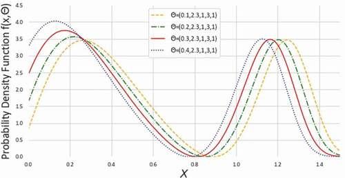
It is immediate from the Figures 1–4 that the density of NEGLED can be decreasing, decreasing-increasing type, unimodal or bimodal depending upon the different values of the parameters.

Figure 1. Density plots of NEGLED model at different values of $\mathrm{\nabla }$ for $\lambda >1$

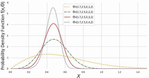
Figure 2. Density plots of NEGLED model at different values of $\mathrm{\nabla }$ for $\lambda <1$

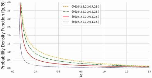
Figure 3. Density plots of NEGLED model at different values of $\mathrm{\nabla }$

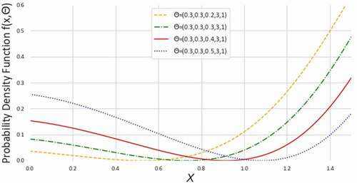
Figure 4. Density plots of NEGLED model at different values of $\mathrm{\nabla }$

From the Figures 5–7, we observe the hazard rate of NEGLED model can be decreasing, increasing, constant or bathtub shaped. Therefore, NEGLED can be used to model the phenomena with constant or non-monotone hazard rates.

Figure 5. The HRFs of NEGLED model at different values of $\mathrm{\nabla }$ for $\lambda >1$

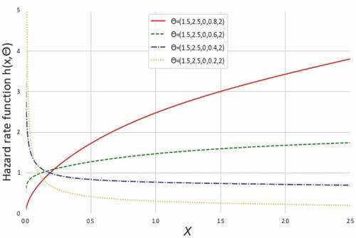
Figure 6. The HRFs of NEGLED model at values of different $\mathrm{\nabla }$ for $\lambda <1$

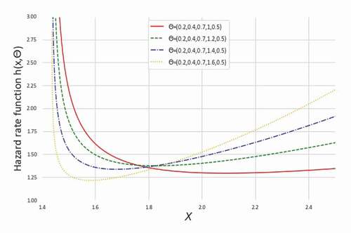
Figure 7. The HRFs of NEGLED model at values of different $\mathrm{\nabla }$

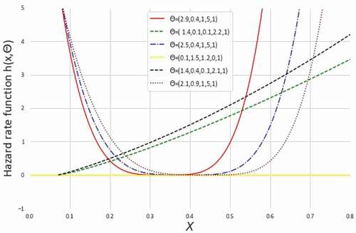
It can easily be shown that through specific parametric substitution, one can get the HRF for ED, RD, GRD, LED, and WD from (2.4). Since GLED is a sub-model of $\mathrm{N}\mathrm{E}\mathrm{G}\mathrm{L}\mathrm{E}\mathrm{D}(\mathrm{\nabla })$ that has the same characteristics of increasing, bathtub-shaped or constant among others HRF for specific values of the parameters. Therefore, in dealing with a diverse range of hazard functions to analyse lifetime data, the NEGLED model demonstrates greater versatility than current literature models.

3. Statistical properties of NEGLED

In this section, we discuss various statistical characteristics of proposed NEGLED model. First, we begin with quantile function as well as random sample generation from NEGLED model. Later on, moments, stress–strength parameters, and order statistics will be discussed consecutively.

3.1. Quantile function and random sample generation

The quantile function which represents the inverse of CDF is given by

$Q(q)=F^{-1}(q).$

Mathematically, the quantile function of $\mathrm{N}\mathrm{E}\mathrm{G}\mathrm{L}\mathrm{E}\mathrm{D}(\mathrm{\nabla })$ can be written as

(3.1) $Q(q)=\frac{-{\theta }_1+\sqrt{{\theta }_1^2+2{\theta }_2\left[{\theta }_3+{\left(-ln(1-q^{\frac{1}{\lambda }})\right)}^{\frac{1}{{\theta }_4}}\right]}}{{\theta }_2},$(3.1)

where $q\sim$ Uniform(0,1). The median of $\mathrm{N}\mathrm{E}\mathrm{G}\mathrm{L}\mathrm{E}\mathrm{D}$ model can be derived by putting $q=0.5$ in Equation (3.1)(3.1) $Q(q)=\frac{-{\theta }_1+\sqrt{{\theta }_1^2+2{\theta }_2\left[{\theta }_3+{\left(-ln(1-q^{\frac{1}{\lambda }})\right)}^{\frac{1}{{\theta }_4}}\right]}}{{\theta }_2},$(3.1) . To generate random sample from $\mathrm{N}\mathrm{E}\mathrm{G}\mathrm{L}\mathrm{E}\mathrm{D}(\mathrm{\nabla })$ model, one can generate it by using the quantile function given in Equation (3.1)(3.1) $Q(q)=\frac{-{\theta }_1+\sqrt{{\theta }_1^2+2{\theta }_2\left[{\theta }_3+{\left(-ln(1-q^{\frac{1}{\lambda }})\right)}^{\frac{1}{{\theta }_4}}\right]}}{{\theta }_2},$(3.1) and a random sample from Uniform(0, 1) distribution. For example, the random sample generation of size $n$ from NEGLED, first generate a random sample $u_1,u_2,\dots ,u_n$ (say) of size $n$ from Uniform(0, 1) distribution. Now replace $q$ with $u_i$ as given in the following formula

$x_i=\frac{-{\theta }_1+\sqrt{{\theta }_1^2+2{\theta }_2\left[{\theta }_3+{\left(-ln(1-u_i^{\frac{1}{\lambda }})\right)}^{\frac{1}{{\theta }_4}}\right]}}{{\theta }_2};i=1,2,\dots ,n.$

3.2. Moments

In pragmatic sciences, moments are important tools for statistical analysis. It can be used to investigate a distribution’s most essential properties (e.g. tendency, dispersion, skewness, and kurtosis). The expression for the moment generating function (MGF), variance, and the $r$th moment of $\mathrm{N}\mathrm{E}\mathrm{G}\mathrm{L}\mathrm{E}\mathrm{D}$ model have been derived in this sub-section.

Theorem 3.1. For the random variable $X$ with $\mathrm{N}\mathrm{E}\mathrm{G}\mathrm{L}\mathrm{E}\mathrm{D}(\mathrm{\nabla })$, i.e. $X\sim \mathrm{N}\mathrm{E}\mathrm{G}\mathrm{L}\mathrm{E}\mathrm{D}(\mathrm{\nabla })$, the $r$th raw moment of $X$ is given by

$\begin{array}{rl}& \mu \mathrm{\prime }r(\mathrm{\nabla })=\lambda \sum _{i=0}^r\sum _{j=0}^{\mathrm{\infty }}\sum _{m=0}^{\mathrm{\infty }}\left(ri\right)\left(\frac{r-i}{2}j\right)\left(\lambda -1\right)(-1{)}^{i+m}{\theta }_1^i\\ & \left[\frac{2^j{({\theta }_1^2+2{\theta }_2{\theta }_3)}^{\frac{r-i}{2}-j}}{{\theta }_2^{r-j}}\right.\end{array}$

$\times \frac{\gamma \left(\frac{j}{{\theta }_4}+1,(m+1){\left(\frac{{\theta }_1^2+2{\theta }_2{\theta }_3}{2{\theta }_2}\right)}^{{\theta }_4}\right)}{{(m+1)}^{\frac{j}{{\theta }_4}+1}}+\frac{2^{\frac{r-i}{2}-j}{({\theta }_1^2+2{\theta }_2{\theta }_3)}^j}{{\theta }_2^{\frac{r+i}{2}+j}}$

(3.2) $\times \left.\frac{\mathrm{\Gamma }\left(\frac{r-i}{2{\theta }_4}-\frac{j}{{\theta }_4}+1,(m+1){\left(\frac{{\theta }_1^2+2{\theta }_2{\theta }_3}{2{\theta }_2}\right)}^{{\theta }_4}\right)}{{(m+1)}^{\frac{r-i}{2{\theta }_4}-\frac{j}{{\theta }_4}+1}}\right].$(3.2)

Proof. We have

$\mu {{ }^{\mathrm{\prime }}}_r(\mathrm{\nabla })={\int }_{\delta }^{\mathrm{\infty }}{x}^{r}f(x;\mathrm{\nabla })\mathrm{d}x$

$=\lambda {\theta }_4{\int }_{\delta }^{\mathrm{\infty }}{x}^r({\theta }_1+{\theta }_{2}x){\left({\theta }_{1}x+\frac{{\theta }_2}{2}{x}^2-{\theta }_3\right)}^{{\theta }_4-1}{e}^{-{\left({\theta }_{1}x+\frac{{\theta }_2}{2}{x}^2-{\theta }_3\right)}^{{\theta }_4}}$

$\times {\left(1-e^{-{\left({\theta }_{1}x+\frac{{\theta }_2}{2}{x}^2-{\theta }_3\right)}^{{\theta }_4}}\right)}^{\lambda -1}\mathrm{d}x.$

Substituting ${\left({\theta }_{1}x+\frac{{\theta }_2}{2}{x}^2-{\theta }_3\right)}^{{\theta }_4}=u$, we get ${\theta }_4({\theta }_1+{\theta }_{2}x){\left({\theta }_{1}x+\frac{{\theta }_2}{2}{x}^2-{\theta }_3\right)}^{{\theta }_4-1}\mathrm{d}x=\mathrm{d}u$.

Since

$x=\frac{-{\theta }_1+\sqrt{{\theta }_1^2+2{\theta }_2{\theta }_3+2{\theta }_2{u}^{1/{\theta }_4}}}{{\theta }_2},$

we have

$\begin{array}{rl}& \mu \mathrm{\prime }r(\mathrm{\nabla })=\lambda {\int }_0^{\mathrm{\infty }}{\left[\frac{-{\theta }_1+\sqrt{{\theta }_1^2+2{\theta }_2{\theta }_3+2{\theta }_2{u}^{1/{\theta }_4}}}{{\theta }_2}\right]}^r\\ & e^{-u}{\left(1-e^{-u}\right)}^{\lambda -1}\mathrm{d}u\end{array}$

$\begin{array}{rl}& =\lambda {\int }_0^{\mathrm{\infty }}\sum _{i=0}^r\left(ri\right)\frac{{(-{\theta }_1)}^i{({\theta }_1^2+2{\theta }_2{\theta }_3+2{\theta }_2{u}^{1/{\theta }_4})}^{\frac{r-i}{2}}}{{\theta }_2^r}\\ & e^{-u}{\left(1-e^{-u}\right)}^{\lambda -1}\mathrm{d}u\end{array}$

$\begin{array}{rl}& =\lambda {\int }_0^{\mathrm{\infty }}\sum _{i=0}^r\left(r_i\right)\frac{{(-{\theta }_1)}^i}{{\theta }_2^r}{\left[1+\frac{{\theta }_1^2+2{\theta }_2{\theta }_3}{2{\theta }_2{u}^{1/{\theta }_4}}\right]}^{\frac{r-i}{2}}\\ & (2{\theta }_2{u}^{1/{\theta }_4}{)}^{\frac{r-i}{2}}{e}^{-u}{\left(1-e^{-u}\right)}^{\lambda -1}\mathrm{d}u.\end{array}$

Suppose $\zeta =\left(\frac{2{\theta }_2}{{\theta }_1^2+2{\theta }_2{\theta }_3}\right)$, it is easy to confirm the below expressions

$\left\{\begin{array}{cc}|\zeta u^{1/{\theta }_4}|<1& \mathrm{i}\mathrm{f}0<u<{\zeta }^{-{\theta }_4}\\ |(\zeta u^{1/{\theta }_4}{)}^{-1}|<1& \mathrm{i}\mathrm{f}{\zeta }^{-{\theta }_4}<u<\mathrm{\infty }\\ \hspace{0.17em}& \hspace{0.17em}\end{array}.\right.$

So, we have

$\begin{array}{rl}& \mu \mathrm{\prime }r(\mathrm{\nabla })=\lambda \sum _{i=0}^r\left(ri\right)\frac{{(-{\theta }_1)}^i}{{\theta }_2^r}{\int }_0^{{\zeta }^{-{\theta }_4}}{\left[1+\frac{1}{\zeta u^{1/{\theta }_4}}\right]}^{\frac{r-i}{2}}\\ & (2{\theta }_2{u}^{1/{\theta }_4}{)}^{\frac{r-i}{2}}{e}^{-u}\sum _{m=0}^{\mathrm{\infty }}\left(\lambda -1\right)(-1{)}^m{e}^{-mu}\mathrm{d}u\end{array}$

$\begin{array}{rl}& +\lambda \sum _{i=0}^r\left(r_i\right)\frac{{(-{\theta }_1)}^i}{{\theta }_2^r}{\int }_{{\zeta }^{-{\theta }_4}}^{\mathrm{\infty }}{\left[1+\frac{1}{\zeta u^{1/{\theta }_4}}\right]}^{\frac{r-i}{2}}(2{\theta }_2{u}^{1/{\theta }_4}{)}^{\frac{r-i}{2}}\\ & e^{-u}\sum _{m=0}^{\mathrm{\infty }}\left(\lambda -1\right)(-1{)}^m{e}^{-mu}\mathrm{d}u\end{array}$

$\begin{array}{rl}& =\lambda \sum _{i=0}^r\sum _{j=0}^{\mathrm{\infty }}\sum _{m=0}^{\mathrm{\infty }}\left(ri\right)\left(\frac{r-i}{2}j\right)\left(\lambda -1\right)(-1{)}^{i+m}\\ & {\theta }_1^i\left[\frac{2^j{({\theta }_1^2+2{\theta }_2{\theta }_3)}^{\frac{r-i}{2}-j}}{{\theta }_2^{r-j}}\right.\end{array}$

$\times \frac{\gamma \left(\frac{j}{{\theta }_4}+1,(m+1){\left(\frac{{\theta }_1^2+2{\theta }_2{\theta }_3}{2{\theta }_2}\right)}^{{\theta }_4}\right)}{{(m+1)}^{\frac{j}{{\theta }_4}+1}}+\frac{2^{\frac{r-i}{2}-j}{({\theta }_1^2+2{\theta }_2{\theta }_3)}^j}{{\theta }_2^{\frac{r+i}{2}+j}}$

$\times \left.\frac{\mathrm{\Gamma }\left(\frac{r-i}{2{\theta }_4}-\frac{j}{{\theta }_4}+1,(m+1){\left(\frac{{\theta }_1^2+2{\theta }_2{\theta }_3}{2{\theta }_2}\right)}^{{\theta }_4}\right)}{{(m+1)}^{\frac{r-i}{2{\theta }_4}-\frac{j}{{\theta }_4}+1}}\right],$

where $\mathrm{\Gamma }(s,t)$ and $\gamma (s,t)$, respectively, denotes the upper incomplete gamma function and lower incomplete gamma function.□

Remark 3.1. The $r^{th}$ raw moment, with shape parameter $2{\theta }_4$ and scale parameter $\sqrt{\frac{2}{{\theta }_2}}$, of the Weibull distribution can be found by putting ${\theta }_1={\theta }_3=0$ and $\lambda =1$ in (3.2).

Lemma 3.1. Let $X\sim \mathrm{N}\mathrm{E}\mathrm{G}\mathrm{L}\mathrm{E}\mathrm{D}(\mathrm{\nabla })$. Then we have

(3.3) $\begin{array}{rl}& \sum _{j=0}^r\sum _{i=0}^{2j}\left(rj\right)\left(2ji\right)\frac{{(-1)}^{r-j}{({\theta }_1^2+2{\theta }_2{\theta }_3)}^{r-j}{\theta }_1^i}{2^r{\theta }_2^{r-2j+i}}\\ & \mu \mathrm{\prime }2j-i(\mathrm{\nabla })=\lambda \sum _{m=0}^{\mathrm{\infty }}\left(\lambda -1\right)(-1{)}^m\frac{\mathrm{\Gamma }\left(\frac{r}{{\theta }_4}+1\right)}{{(m+1)}^{\frac{r}{{\theta }_4}+1}}.\end{array}$(3.3)

Proof.

$E\left[{\left({\theta }_{1}X+\frac{{\theta }_2}{2}{X}^2-{\theta }_3\right)}^r\right]=E\left[{\xi }^r(X)\right]$

$={\theta }_4\lambda {\int }_{\delta }^{\mathrm{\infty }}\xi { }^{\mathrm{\prime }}(x){\xi }^{r+{\theta }_4-1}(x)e^{-{\xi }^{{\theta }_4}(x)}{\left(1-e^{-{\xi }^{{\theta }_4}(x)}\right)}^{\lambda -1}\mathrm{d}x$

Substituting $u={\xi }^{{\theta }_4}(x)$, on taking derivative we get $\mathrm{d}u={\theta }_4\xi { }^{\mathrm{\prime }}(x){\xi }^{{\theta }_4-1}(x)\mathrm{d}x$. So,

$E\left[{\left({\theta }_{1}X+\frac{{\theta }_2}{2}{X}^2-{\theta }_3\right)}^r\right]={\int }_0^{\mathrm{\infty }}{u}^{\frac{r}{{\theta }_4}}{e}^{-u}{\left(1-e^{-u}\right)}^{\lambda -1}\mathrm{d}u$

(3.4) $=\lambda \sum _{m=0}^{\mathrm{\infty }}\left(\lambda -1\right)(-1{)}^m\frac{\mathrm{\Gamma }\left(\frac{r}{{\theta }_4}+1\right)}{{(m+1)}^{\frac{r}{{\theta }_4}+1}}.$(3.4)

Using binomially expansion in the left hand side of (3.4), we have

$\begin{array}{rl}& E\left[\sum _{j=0}^r\sum _{i=0}^{2j}\left(r_j\right)\left(2ji\right)\frac{{(-1)}^{r-j}{({\theta }_1^2+2{\theta }_2{\theta }_3)}^{r-j}{\theta }_1^i}{2^r{\theta }_2^{r-2j+i}}{X}^{2j-i}\right]\\ & =\lambda \sum _{m=0}^{\mathrm{\infty }}\left(\lambda -1\right)(-1{)}^m\frac{\mathrm{\Gamma }\left(\frac{r}{{\theta }_4}+1\right)}{{(m+1)}^{\frac{r}{{\theta }_4}+1}}\end{array}$

$\begin{array}{rl}& \Rightarrow \sum _{j=0}^r\sum _{i=0}^{2j}\left(r{\hspace{0.17em}}_j\right)\left(2ji\right)\frac{{(-1)}^{r-j}{({\theta }_1^2+2{\theta }_2{\theta }_3)}^{r-j}{\theta }_1^i}{2^r{\theta }_2^{r-2j+i}}\mu \mathrm{\prime }2j-i(\mathrm{\nabla })\\ & =\lambda \sum _{m=0}^{\mathrm{\infty }}\left(\lambda -1\right)(-1{)}^m\frac{\mathrm{\Gamma }\left(\frac{r}{{\theta }_4}+1\right)}{{(m+1)}^{\frac{r}{{\theta }_4}+1}},\end{array}$

which proves the result.□

Theorem 3.2. The variance of NEGLED model is derived as follow

(3.5) $\mathrm{V}\mathrm{a}\mathrm{r}(X)={\sigma }^2=\frac{2}{{\theta }_2}\left[\begin{array}{c}\lambda \sum _{m=0}^{\mathrm{\infty }}\left(\lambda -1\right)(-1{)}^m\frac{\mathrm{\Gamma }(\frac{1}{{\theta }_4}+1)}{{(m+1)}^{\frac{1}{{\theta }_4}+1}}\\ -{\theta }_1\mu +{\theta }_3-\frac{{\theta }_2}{2}{\mu }^2\end{array}\right],$(3.5)

where $\mu$ is the mean of $X$, which can be derived by substituting $r=1$ in (3.2).

Proof. Simply placing $r=1$ in (3.3), we get

$\mu \mathrm{\prime }2(\mathrm{\nabla })=\frac{2}{{\theta }_2}\left[\lambda \sum _{m=0}^{\mathrm{\infty }}\left(\lambda -1\hspace{0.17em}\right){(-1)}^m\frac{\mathrm{\Gamma }\left(\frac{1}{{\theta }_4}+1\right)}{{(m+1)}^{\frac{1}{{\theta }_4}+1}}-{\theta }_1\mu +{\theta }_3\right],$

where $\mu$ is the mean of the random variable $X$. Also, it is easy to get $\mu {{ }^{\mathrm{\prime }}}_2(\mathrm{\nabla })$ on putting $r=1$ in (3.4) as follow

$E\left[{\theta }_{1}X+\frac{{\theta }_2}{2}{X}^2-{\theta }_3\right]=\lambda \sum _{m=0}^{\mathrm{\infty }}\left(\lambda -1\right)(-1{)}^m\frac{\mathrm{\Gamma }\left(\frac{1}{{\theta }_4}+1\right)}{{(m+1)}^{\frac{1}{{\theta }_4}+1}}$

$\begin{array}{rl}& \Rightarrow {\theta }_1\mu +\frac{{\theta }_2}{2}\mu \mathrm{\prime }2(\mathrm{\nabla })-{\theta }_3\\ & =\lambda \sum _{m=0}^{\mathrm{\infty }}\left(\lambda -1\right)(-1{)}^m\frac{\mathrm{\Gamma }\left(\frac{1}{{\theta }_4}+1\right)}{{(m+1)}^{\frac{1}{{\theta }_4}+1}}\end{array}$

$\begin{array}{rl}& \Rightarrow \mu \mathrm{\prime }2(\mathrm{\nabla })=\frac{2}{{\theta }_2}\\ & \left[\lambda \sum _{m=0}^{\mathrm{\infty }}\left(\lambda -1\right){(-1)}^m\frac{\mathrm{\Gamma }\left(\frac{1}{{\theta }_4}+1\right)}{{(m+1)}^{\frac{1}{{\theta }_4}+1}}-{\theta }_1\mu +{\theta }_3\right].\end{array}$

So, the variance of $\mathrm{N}\mathrm{E}\mathrm{G}\mathrm{L}\mathrm{E}(\mathrm{\nabla })$ distribution is derived as follow

$Var(X)=\mu {{ }^{\mathrm{\prime }}}_2(\mathrm{\nabla })-{\mu }^2$

$=\frac{2}{{\theta }_2}\left[\begin{array}{c}\lambda \sum _{m=0}^{\mathrm{\infty }}\left(\lambda -1\right)(-1{)}^m\frac{\mathrm{\Gamma }\left(\frac{1}{{\theta }_4}+1\right)}{{(m+1)}^{\frac{1}{{\theta }_4}+1}}\\ -{\theta }_1\mu +{\theta }_3-\frac{{\theta }_2}{2}{\mu }^2\end{array}\right].$

□

Theorem 3.3. Suppose $X$ has a $\mathrm{N}\mathrm{E}\mathrm{G}\mathrm{L}\mathrm{E}\mathrm{D}(\mathrm{\nabla })$ distribution, then the MGF, i.e. $M_X(s)$, of $X$ is given by

$\begin{array}{rl}& M_X(s)=\lambda \sum _{r=0}^{\mathrm{\infty }}\sum _{i=0}^r\sum _{j=0}^{\mathrm{\infty }}\sum _{m=0}^{\mathrm{\infty }}\left(r_i\right)\left(\underset{j}{\frac{r-i}{2}}\right)\left(\lambda -1\right)(-1{)}^{i+m}\\ & {\theta }_1^i\frac{t^r}{r!}\left[\frac{2^j{({\theta }_1^2+2{\theta }_2{\theta }_3)}^{\frac{r-i}{2}-j}}{{\theta }_2^{r-j}}\right.\end{array}$

$\times \frac{\gamma \left(\frac{j}{{\theta }_4}+1,(m+1){\left(\frac{{\theta }_1^2+2{\theta }_2{\theta }_3}{2{\theta }_2}\right)}^{{\theta }_4}\right)}{{(m+1)}^{\frac{j}{{\theta }_4}+1}}+\frac{2^{\frac{r-i}{2}-j}{({\theta }_1^2+2{\theta }_2{\theta }_3)}^j}{{\theta }_2^{\frac{r+i}{2}+j}}$

$\times \left.\frac{\mathrm{\Gamma }\left(\frac{r-i}{2{\theta }_4}-\frac{j}{{\theta }_4}+1,(m+1){\left(\frac{{\theta }_1^2+2{\theta }_2{\theta }_3}{2{\theta }_2}\right)}^{{\theta }_4}\right)}{{(m+1)}^{\frac{r-i}{2{\theta }_4}-\frac{j}{{\theta }_4}+1}}\right].$

Proof. By definition of the MGF of $X$, we have

$M_X(s)=E[e^{sX}]$

$=E\left[\sum _{r=0}^{\mathrm{\infty }}\frac{{(sX)}^r}{r!}\right]$

$=\sum _{r=0}^{\mathrm{\infty }}\frac{s^r{\mu { }^{\mathrm{\prime }}}_r(\mathrm{\nabla })}{r!}$

$\begin{array}{rl}& =\lambda \sum _{r=0}^{\mathrm{\infty }}\sum _{i=0}^r\sum _{j=0}^{\mathrm{\infty }}\sum _{m=0}^{\mathrm{\infty }}\left(r_i\right)\left(\frac{r-i}{2}j\right)\left(\lambda -1\right)(-1{)}^{i+m}\\ & {\theta }_1^i\frac{t^r}{r!}\left[\frac{2^j{({\theta }_1^2+2{\theta }_2{\theta }_3)}^{\frac{r-i}{2}-j}}{{\theta }_2^{r-j}}\right.\end{array}$

$\times \frac{\gamma \left(\frac{j}{{\theta }_4}+1,(m+1){\left(\frac{{\theta }_1^2+2{\theta }_2{\theta }_3}{2{\theta }_2}\right)}^{{\theta }_4}\right)}{{(m+1)}^{\frac{j}{{\theta }_4}+1}}+\frac{2^{\frac{r-i}{2}-j}{({\theta }_1^2+2{\theta }_2{\theta }_3)}^j}{{\theta }_2^{\frac{r+i}{2}+j}}$

$\times \left.\frac{\mathrm{\Gamma }\left(\frac{r-i}{2{\theta }_4}-\frac{j}{{\theta }_4}+1,(m+1){\left(\frac{{\theta }_1^2+2{\theta }_2{\theta }_3}{2{\theta }_2}\right)}^{{\theta }_4}\right)}{{(m+1)}^{\frac{r-i}{2{\theta }_4}-\frac{j}{{\theta }_4}+1}}\right].$

□

3.3. Stress–strength parameter

Let random stress and strength of the component are denoted by $X$ and $Y$, respectively. Then $R=P(Y<X)$ is known as the stress–strength parameter, which describes the measure of component’s reliability. Let $X\sim \mathrm{N}\mathrm{E}\mathrm{G}\mathrm{L}\mathrm{E}\mathrm{D}({\theta }_1,{\theta }_2,{\theta }_3,{\theta }_4,{\lambda }_1)$ and $Y\sim \mathrm{N}\mathrm{E}\mathrm{G}\mathrm{L}\mathrm{E}\mathrm{D}({\theta }_1,{\theta }_2,{\theta }_3,{\theta }_4,{\lambda }_2)$ be two independent random variables. Then

(3.6) $R=P(Y<X)=\frac{{\lambda }_1}{{\lambda }_1+{\lambda }_2}.$(3.6)

Proof.

$\begin{array}{rl}& P(YX)={\int }_{\delta }^{\mathrm{\infty }}\left({\int }_{\delta }^{x}f(y;{\theta }_1,{\theta }_2,{\theta }_3,{\theta }_4,{\lambda }_2)\mathrm{d}y\right)f\\ & (x;{\theta }_1,{\theta }_2,{\theta }_3,{\theta }_4,{\lambda }_1)\mathrm{d}x\end{array}$

$={\lambda }_1{\lambda }_2{\theta }_4^2{\int }_{\delta }^{\mathrm{\infty }}\xi { }^{\mathrm{\prime }}(x){\xi }^{{\theta }_4-1}(x)e^{-{\xi }^{{\theta }_4}(x)}{\left(1-e^{-{\xi }^{{\theta }_4}(x)}\right)}^{{\lambda }_1-1}$

$\times \left({\int }_{\delta }^x\xi { }^{\mathrm{\prime }}(y){\xi }^{{\theta }_4-1}(y)e^{-{\xi }^{{\theta }_4}(y)}{\left(1-e^{-{\xi }^{{\theta }_4}(y)}\right)}^{{\lambda }_2-1}\mathrm{d}y\right)\mathrm{d}x.$

Consider the transformation $u=e^{-{\xi }^{{\theta }_4}(y)}$, which implies that $\mathrm{d}u=-{\theta }_4\xi { }^{\mathrm{\prime }}(y){\xi }^{{\theta }_4-1}(y)e^{-{\xi }^{{\theta }_4}(y)}\mathrm{d}y$. So

$\begin{array}{rl}& P(YX)={\lambda }_1{\lambda }_2{\theta }_4{\int }_{\delta }^{\mathrm{\infty }}\xi \mathrm{\prime }(x){\xi }^{{\theta }_4-1}(x)e^{-{\xi }^{{\theta }_4}(x)}\\ & {\left(1-e^{-{\xi }^{{\theta }_4}(x)}\right)}^{{\lambda }_1-1}\left({\int }_{e^{-{\xi }^{{\theta }_4}(x)}}^1{(1-u)}^{{\lambda }_2-1}\mathrm{d}u\right)\mathrm{d}x\end{array}$

$=-{\lambda }_1{\theta }_4{\int }_{\delta }^{\mathrm{\infty }}\xi { }^{\mathrm{\prime }}(x){\xi }^{{\theta }_4-1}(x)e^{-{\xi }^{{\theta }_4}(x)}{\left(1-e^{-{\xi }^{{\theta }_4}(x)}\right)}^{{\lambda }_1+{\lambda }_2-1}\mathrm{d}x.$

Now, take $s=\frac{1}{e^{{\xi }^{{\theta }_4}(x)}}$, we get $\mathrm{d}s=\frac{-{\theta }_4\xi { }^{\mathrm{\prime }}(x){\xi }^{{\theta }_4}(x)}{\xi (x)e^{{\xi }^{{\theta }_4}(x)}}\mathrm{d}x$. So

$P(Y<X)=-{\lambda }_1{\int }_0^1(1-s{)}^{{\lambda }_1+{\lambda }_2-1}\mathrm{d}s$

$=\frac{{\lambda }_1}{{\lambda }_1+{\lambda }_2}.$

3.4. Order statistics

Let $X_{(1)}\le X_{(2)}\le \cdots \le X_{(m)}$ denote the order statistics of the random sample $X_1,X_2,\dots ,X_m$ from $\mathrm{N}\mathrm{E}\mathrm{G}\mathrm{L}\mathrm{E}\mathrm{D}(\mathrm{\nabla })$ model. Then, using the standard formula of the PDF of $k^{th}$ order statistics see Arnold et al. (1992)), the PDF of the $k^{th}$ order statistic $X_{(k)}$ is

$\begin{array}{rl}& f_{X_{(k)}}(x;\mathrm{\nabla })=\frac{m!}{(k-1)!(m-k)!}\lambda {\theta }_4\xi \mathrm{\prime }(x){\xi }^{{\theta }_4-1}\\ & (x)e^{-{\xi }^{{\theta }_4}(x)}{\left(1-e^{-{\xi }^{{\theta }_4}(x)}\right)}^{\lambda k-1}\end{array}$

$\times {\left(1-{\left(1-e^{-{\xi }^{{\theta }_4}(x)}\right)}^{\lambda }\right)}^{m-k};x>\delta .$

Thus, the PDF of $X_{(1)}$ (the smallest order statistic) is

$\begin{array}{rl}& f_{X_{(1)}}(x;\mathrm{\nabla })=m{\theta }_4\lambda \xi \mathrm{\prime }(x){\xi }^{{\theta }_4-1}(x)e^{-{\xi }^{{\theta }_4}(x)}\\ & {\left(1-e^{-{\xi }^{{\theta }_4}(x)}\right)}^{\lambda -1}{\left(1-{\left(1-e^{-{\xi }^{{\theta }_4}(x)}\right)}^{\lambda }\right)}^{m-1},x\delta ,\end{array}$

and the PDF of $X_{(m)}$ (the largest order statistic) is

$f_{X_{(m)}}(x;\mathrm{\nabla })=m{\theta }_4\lambda \xi { }^{\mathrm{\prime }}(x){\xi }^{{\theta }_4-1}(x)e^{-{\xi }^{{\theta }_4}(x)}{\left(1-e^{-{\xi }^{{\theta }_4}(x)}\right)}^{m\lambda -1},x>\delta .$

Theorem 3.4. Let $X_k\sim \mathrm{N}\mathrm{E}\mathrm{G}\mathrm{L}\mathrm{E}\mathrm{D}({\theta }_1,{\theta }_2,{\theta }_3,{\theta }_4,{\lambda }_k)$ for $1\le k$ be independent r.v.’s. Then $X_{(m)}\sim \mathrm{N}\mathrm{E}\mathrm{G}\mathrm{L}\mathrm{E}\mathrm{D}({\theta }_1,{\theta }_2,{\theta }_3,{\theta }_4,{\sum }_{k=1}^m{\lambda }_k)$.

The proof of Theorem 3.4 is simple and hence omitted.

The joint PDF of $X_{(k)}$ and $X_{(l)}$ is now calculated using the standard formula of the joint PDF of two order statistics (see Arnold et al., 1992) as

$\begin{array}{rl}& f_{X_{(k)}{X}_{(l)}}(x_k,x_l;\mathrm{\nabla })=M{\theta }_4^2{\lambda }^2\xi \mathrm{\prime }(x_k)\xi \mathrm{\prime }(x_l)(\xi (x_k)\xi (x_l){)}^{{\theta }_4-1}\\ & e^{-{\xi }_4^{\theta }(x_k)-{\xi }_4^{\theta }(x_l)}{\left(1-e^{-{\xi }^{{\theta }_4}(x_k)}\right)}^{\lambda k-1}\end{array}$

$\begin{array}{rl}& \times {\left(1-e^{-{\xi }^{{\theta }_4}(x_l)}\right)}^{\lambda -1}{\left(\begin{array}{c}{\left(1-e^{-{\xi }^{{\theta }_4}(x_l)}\right)}^{\lambda }-\\ {\left(1-e^{-{\xi }^{{\theta }_4}(x_k)}\right)}^{\lambda }\end{array}\right)}^{l-k-1}\\ & {\left(1-{\left(1-e^{-{\xi }^{{\theta }_4}(x_k)}\right)}^{\lambda }\right)}^{m-l},\end{array}$

where $M=\frac{m!}{(k-1)!(l-k-1)!(m-l)!}$. Then, for NEGLED, the joint density of $X_{(1)}$ and $X_{(m)}$ becomes of the form

$\begin{array}{rl}& f_{X_{(1)}{X}_{(m)}}(x_1,x_m;\mathrm{\nabla })=m(m-1){\theta }_4^2{\lambda }^2\xi \mathrm{\prime }(x_1)\xi \mathrm{\prime }(x_m)(\xi (x_1)\\ & \xi (x_m){)}^{{\theta }_4-1}{e}^{-{\xi }_4^{\theta }(x_1)-{\xi }_4^{\theta }(x_m)}\end{array}$

$\begin{array}{rl}& \times {\left[\left(1-e^{-{\xi }^{{\theta }_4}(x_1)}\right)\left(1-e^{-{\xi }^{{\theta }_4}(x_m)}\right)\right]}^{\lambda -1}\\ & {\left[{\left(1-e^{-{\xi }^{{\theta }_4}(x_m)}\right)}^{\lambda }-{\left(1-e^{-{\xi }^{{\theta }_4}(x_1)}\right)}^{\lambda }\right]}^{m-2}.\end{array}$

4. Statistcal inference

Now, we discuss the estimation of the model parameters by using the method of maximum likelihood estimation. Let draw a random sample of size $m$, i.e. $\mathbf{x}=(x_1,x_2,\dots ,x_m)$, from $\mathrm{N}\mathrm{E}\mathrm{G}\mathrm{L}\mathrm{E}\mathrm{D}(\mathrm{\nabla })$. The likelihood function $L(\mathrm{\nabla };\mathbf{x})$ for $\mathrm{\nabla }$ is given by

$L(\mathrm{\nabla };\mathbf{x})=\prod _{k=1}^{m}f(x_k;\mathrm{\nabla })={\theta }_4^m{\lambda }^m\prod _{k=1}^m\xi { }^{\mathrm{\prime }}(x_k){\xi }^{{\theta }_4-1}(x_k)e^{-{\xi }_4^{\theta }(x_k)}{\left(1-e^{-{\xi }_4^{\theta }(x_k)}\right)}^{\lambda -1}$

and corresponding log-likelihood functions $l(\mathrm{\nabla };\mathbf{x})$ of above equation is

$l(\mathrm{\nabla };\mathbf{x})=mln{\theta }_4+mln\lambda +\sum _{k=1}^{m}ln\xi { }^{\mathrm{\prime }}(x_k)+({\theta }_4-1)\sum _{k=1}^{m}ln\xi (x_k)-\sum _{k=1}^m{\xi }_4^{\theta }(x_k)$

$+(\lambda -1)\sum _{k=1}^{m}ln\left(1-e^{-{\xi }_4^{\theta }(x_k)}\right).$

First, differentiate the log-likelihood function with respect to unknown parameters and equate it to 0. The normal equations are given as

$\frac{\mathrm{\partial }l(\mathrm{\nabla };\mathbf{x})}{\mathrm{\partial }{\theta }_1}=\sum _{k=1}^m\frac{1}{{\theta }_2{x}_k+{\theta }_1}+2({\theta }_4-1)\sum _{k=1}^m\frac{x_k}{{\theta }_2{x}_k^2+2{\theta }_1{x}_k-2{\theta }_3}-\frac{{\theta }_4}{2^{{\theta }_4-1}}\times$

(4.1) $\sum _{k=1}^m{x}_k({\theta }_2{x}_k^2+2{\theta }_1{x}_k-2{\theta }_3{)}^{{\theta }_4-1}\left(\frac{1-\lambda e^{-{\left(\frac{{\theta }_2}{2}{x}_k^2+{\theta }_1{x}_k-{\theta }_3\right)}_4^{\theta }}}{1-e^{-{\left(\frac{{\theta }_2}{2}{x}_k^2+{\theta }_1{x}_k-{\theta }_3\right)}_4^{\theta }}}\right)=0,$(4.1)

$\frac{\mathrm{\partial }l(\mathrm{\nabla };\mathbf{x})}{\mathrm{\partial }{\theta }_2}=\sum _{k=1}^m\frac{x_k}{{\theta }_2{x}_k+{\theta }_1}+({\theta }_4-1)\sum _{k=1}^m\frac{x_k^2}{{\theta }_2{x}_k^2+2{\theta }_1{x}_k-2{\theta }_3}-\frac{{\theta }_4}{2^{{\theta }_4}}\times$

(4.2) $\sum _{k=1}^m{x}_k^2({\theta }_2{x}_k^2+2{\theta }_1{x}_k-2{\theta }_3{)}^{{\theta }_4-1}\left(\frac{1-\lambda e^{-{\left(\frac{{\theta }_2}{2}{x}_k^2+{\theta }_1{x}_k-{\theta }_3\right)}_4^{\theta }}}{1-e^{-{\left(\frac{{\theta }_2}{2}{x}_k^2+{\theta }_1{x}_k-{\theta }_3\right)}_4^{\theta }}}\right)=0,$(4.2)

$\frac{\mathrm{\partial }l(\mathrm{\nabla };\mathbf{x})}{\mathrm{\partial }{\theta }_3}=-2({\theta }_4-1)\sum _{k=1}^m\frac{1}{{\theta }_2{x}_k^2+2{\theta }_1{x}_k-2{\theta }_3}+\frac{{\theta }_4}{2^{{\theta }_4-1}}\times$

(4.3) $\sum _{k=1}^m({\theta }_2{x}_k^2+2{\theta }_1{x}_k-2{\theta }_3{)}^{{\theta }_4-1}\left(\frac{1-\lambda e^{-{\left(\frac{{\theta }_2}{2}{x}_k^2+{\theta }_1{x}_k-{\theta }_3\right)}_4^{\theta }}}{1-e^{-{\left(\frac{{\theta }_2}{2}{x}_k^2+{\theta }_1{x}_k-{\theta }_3\right)}_4^{\theta }}}\right)=0,$(4.3)

$\frac{\mathrm{\partial }l(\mathrm{\nabla };\mathbf{x})}{\mathrm{\partial }{\theta }_4}=\frac{m}{{\theta }_4}+\sum _{k=1}^{m}ln\left(\frac{{\theta }_2}{2}{x}_k^2+{\theta }_1{x}_k-{\theta }_3\right)-\frac{1}{2^{{\theta }_4}}\sum _{k=1}^m({\theta }_2{x}_k^2+2{\theta }_1{x}_k-2{\theta }_3{)}^{{\theta }_4}$

(4.4) $\times ln\left(\frac{{\theta }_2}{2}{x}_k^2+{\theta }_1{x}_k-{\theta }_3\right)\left(\frac{1-\lambda e^{-{\left(\frac{{\theta }_2}{2}{x}_k^2+{\theta }_1{x}_k-{\theta }_3\right)}_4^{\theta }}}{1-e^{-{\left(\frac{{\theta }_2}{2}{x}_k^2+{\theta }_1{x}_k-{\theta }_3\right)}_4^{\theta }}}\right)=0,$(4.4)

(4.5) $\frac{\mathrm{\partial }l(\mathrm{\nabla };\mathbf{x})}{\mathrm{\partial }\lambda }=\frac{m}{\lambda }+\sum _{k=1}^{m}ln\left(1-e^{-{\left(\frac{{\theta }_2}{2}{x}_k^2+{\theta }_1{x}_k-{\theta }_3\right)}_4^{\theta }}\right)=0.$(4.5)

Since the MLEs of $\mathrm{N}\mathrm{E}\mathrm{G}\mathrm{L}\mathrm{E}\mathrm{D}(\mathrm{\nabla })$ cannot be obtained in a closed form, one can use iterative procedures like Newton–Raphson method to compute them. It would be impossible to determine the exact distributions of the MLE’s of the parameters due to lack of closed form solution.

The solution to the aforementioned non-linear Equations (4.1(4.1) $\sum _{k=1}^m{x}_k({\theta }_2{x}_k^2+2{\theta }_1{x}_k-2{\theta }_3{)}^{{\theta }_4-1}\left(\frac{1-\lambda e^{-{\left(\frac{{\theta }_2}{2}{x}_k^2+{\theta }_1{x}_k-{\theta }_3\right)}_4^{\theta }}}{1-e^{-{\left(\frac{{\theta }_2}{2}{x}_k^2+{\theta }_1{x}_k-{\theta }_3\right)}_4^{\theta }}}\right)=0,$(4.1) )–(4.5(4.5) $\frac{\mathrm{\partial }l(\mathrm{\nabla };\mathbf{x})}{\mathrm{\partial }\lambda }=\frac{m}{\lambda }+\sum _{k=1}^{m}ln\left(1-e^{-{\left(\frac{{\theta }_2}{2}{x}_k^2+{\theta }_1{x}_k-{\theta }_3\right)}_4^{\theta }}\right)=0.$(4.5) ) are determined using simulation in R software, assuming asymptotic distribution based on large sample approximations. In our case, $\mathrm{N}\mathrm{E}\mathrm{G}\mathrm{L}\mathrm{E}\mathrm{D}(\mathrm{\nabla })$ asymptotically follows ${\mathcal{N}}_5(\mathrm{\nabla },B(\hat{\mathrm{\nabla }}))$. Where $\hat{\mathrm{\nabla }}=({\hat{\theta }}_1,{\hat{\theta }}_2,{\hat{\theta }}_3,{\hat{\theta }}_4,\hat{\lambda })$ is the vector of MLE’s and denotes the mean vector $\mathrm{\nabla }$ meanwhile $B(\hat{\mathrm{\nabla }})$ denotes the dispersion matrix. Particularly, based on a sample of size $m$, as $m\to \mathrm{\infty }$, we have $(\hat{\mathrm{\nabla }}-\mathrm{\nabla })d{\mathcal{N}}_5(0,B(\hat{\mathrm{\nabla }})),$ where $0=(0,0,0,0,0){ }^{\mathrm{\prime }}$ and $B(\hat{\mathrm{\nabla }})=W^{-1}(\hat{\mathrm{\nabla }})$, the inverse of the observed information matrix $W(\hat{\mathrm{\nabla }})=(a_{kp})$ for $1\le k,p\le 5$. Suppose $({\theta }_1,{\theta }_2,{\theta }_3,{\theta }_4,\lambda )=({\vartheta }_1,{\vartheta }_2,{\vartheta }_3,{\vartheta }_4,{\vartheta }_5)$. Then, for $1\le k<p\le 5$, we obtain $a_{kp}=-\frac{{\mathrm{\partial }}^{2}l(x;\hat{\mathrm{\nabla }})}{\mathrm{\partial }{\hat{\vartheta }}_k\mathrm{\partial }{\hat{\vartheta }}_p}$, $a_{kk}=-\frac{{\mathrm{\partial }}^{2}l(x;\hat{\mathrm{\nabla }})}{\mathrm{\partial }{\hat{\vartheta }}_k^2}$ and $a_{kp}=a_{pk}$. Also, $Cov({\hat{\vartheta }}_k,{\hat{\vartheta }}_p)=d_{kp}$, $Var({\hat{\vartheta }}_k)=d_{kk}$ and $d_{kp}=d_{pk}$, where $B(\hat{\mathrm{\nabla }})=(d_{kp})$. Thus, from normal Equations (4.1(4.1) $\sum _{k=1}^m{x}_k({\theta }_2{x}_k^2+2{\theta }_1{x}_k-2{\theta }_3{)}^{{\theta }_4-1}\left(\frac{1-\lambda e^{-{\left(\frac{{\theta }_2}{2}{x}_k^2+{\theta }_1{x}_k-{\theta }_3\right)}_4^{\theta }}}{1-e^{-{\left(\frac{{\theta }_2}{2}{x}_k^2+{\theta }_1{x}_k-{\theta }_3\right)}_4^{\theta }}}\right)=0,$(4.1) )–(4.5(4.5) $\frac{\mathrm{\partial }l(\mathrm{\nabla };\mathbf{x})}{\mathrm{\partial }\lambda }=\frac{m}{\lambda }+\sum _{k=1}^{m}ln\left(1-e^{-{\left(\frac{{\theta }_2}{2}{x}_k^2+{\theta }_1{x}_k-{\theta }_3\right)}_4^{\theta }}\right)=0.$(4.5) ), we can calculate the elements of $B(\hat{\mathrm{\nabla }})$. The quantity $\left({\hat{\vartheta }}_k\pm z_{\alpha /2}SE({\hat{\vartheta }}_k)\right)$ represents the $100(1-\alpha )\mathrm{\%}$ confidence interval of ${\vartheta }_k$, where $z_{\alpha /2}$ denotes the upper $\alpha /2$-th percentile of the standard normal distribution and $\alpha$ denotes the level of significance.

To study various properties of MLE, the estimates of parameters of NEGLED model are derived using simulation. Samples of size $20(20)100$ are considered with iteration of 10,000 from $\mathrm{N}\mathrm{E}\mathrm{G}\mathrm{L}\mathrm{E}\mathrm{D}(5.2,2.5,7.8,1.6,0.7)$ using optim command in R software. The bias, standard error, and coverage length (length of $95\mathrm{\%}$ confidence interval) for the MLE of each parameter are evaluated for each case. Findings are presented in the Table 2.

Table 2. Bias, Standard error (SE), and Coverage length (CL) for MLEs from NEGLED model

Size of the sample ($n$)		${\hat{\theta }}_1$	${\hat{\theta }}_2$	${\hat{\theta }}_3$	${\hat{\theta }}_4$	$\hat{\lambda }$
	Bias	−0.0416	−0.2146	−0.1819	−0.0113	0.0454
20	SE	0.1184	0.1957	0.2723	0.0697	0.0681
	CL	0.4640	0.7673	1.0673	0.2732	0.2669
	Bias	−0.0236	−0.2113	−0.1147	0.1234	−0.0771
40	SE	0.0352	0.0288	0.0666	0.0577	0.0206
	CL	0.1380	0.1130	0.2609	0.2174	0.0807
	Bias	−0.0122	−0.2057	−0.1418	0.1298	−0.1006
60	SE	0.0116	0.0214	0.0286	0.0553	0.0128
	CL	0.0456	0.0838	0.1121	0.2167	0.0500
	Bias	−0.0125	−0.2062	−0.1285	0.1148	−0.0929
80	SE	0.0082	0.0095	0.0178	0.0246	0.0080
	CL	0.0322	0.0371	0.0699	0.0965	0.0312
	Bias	0.0117	−0.1900	−0.0752	0.2073	−0.0457
100	SE	0.0029	0.0020	0.0028	0.0194	0.0076
	CL	0.0115	0.0077	0.0109	0.0762	0.0299

We noticed that perhaps the standard errors, coverage lengths, and absolute biases of each of the ${\hat{\theta }}_1$, ${\hat{\theta }}_2$, ${\hat{\theta }}_3$, ${\hat{\theta }}_4$ and $\hat{\lambda }$ MLE’s decrease as increasing the size of the sample, see Table 2. This indicates that the MLE method provides good estimates of the parameters for the NEGLED model.

Further, we estimate the stress–strength parameter i.e. $R$. In the context of the reliability of a system, it is very important to study the system performance referred to as the stress–strength parameter. The system will only survive if the applied stress is lesser than the strength. In practise, a good design is one in which the strength is always greater than the expected stress. In the statistical sciences, inferring the stress–strength parameter from a complete or censored sample has piqued the interest of many scientists over years, and the challenge of estimating $R$ under various scenarios has been extensively researched. Many research on the inference of stress–strength parameter $R$ from various perspective have recently been published in the literature. For example, half logistic distribution (Ratnam et al., 2000), Burr type X distribution (Kim et al., 2000), and normal distribution (Guo and Krishnamoorthy (2004), Barbiero (2011)).

Let we draw two independent random samples, i.e. $\mathbf{x}=(x_1,\dots ,x_m)$ and $\mathbf{y}=(y_1,\dots ,y_n)$, from $\mathrm{N}\mathrm{E}\mathrm{G}\mathrm{L}\mathrm{E}\mathrm{D}({\theta }_1,{\theta }_2,{\theta }_3,{\theta }_4,{\lambda }_1)$ and $\mathrm{N}\mathrm{E}\mathrm{G}\mathrm{L}\mathrm{E}\mathrm{D}({\theta }_1,{\theta }_2,{\theta }_3,{\theta }_4,{\lambda }_2)$ of sizes $m$ and $n$ respectively. Then the log-likelihood function $l(\mathrm{{\rm Y}};\mathbf{x},\mathbf{y})$ of $\mathrm{{\rm Y}}=({\theta }_1,{\theta }_2,{\theta }_3,{\theta }_4,{\lambda }_1,{\lambda }_2)$ is

$l(\mathrm{{\rm Y}};\mathbf{x},\mathbf{y})=(m+n)ln({\theta }_4\lambda )+\sum _{k=1}^{m}ln\xi { }^{\mathrm{\prime }}(x_k)+({\theta }_4-1)\sum _{k=1}^{m}ln\xi (x_k)-\sum _{k=1}^m{\xi }_4^{\theta }(x_k)$

$+({\lambda }_1-1)\sum _{k=1}^{m}ln\left(1-e^{-{\xi }_4^{\theta }(x_k)}\right)+\sum _{k=1}^{n}ln\xi { }^{\mathrm{\prime }}(y_k)+({\theta }_4-1)\sum _{k=1}^{n}ln\xi (y_k)$

$-\sum _{k=1}^n{\xi }_4^{\theta }(y_k)+({\lambda }_2-1)\sum _{k=1}^{n}ln\left(1-e^{-{\xi }_4^{\theta }(y_k)}\right).$

Equations (4.6(4.6) $\begin{array}{rl}& \times \sum _{k=1}^n{y}_k({\theta }_2{y}_k^2+2{\theta }_1{y}_k-2{\theta }_3{)}^{{\theta }_4-1}\\ & \left(\frac{1-{\lambda }_2{e}^{-{\left(\frac{{\theta }_2}{2}{y}_k^2+{\theta }_1{y}_k-{\theta }_3\right)}_4^{\theta }}}{1-e^{-{\left(\frac{{\theta }_2}{2}{y}_k^2+{\theta }_1{y}_k-{\theta }_3\right)}_4^{\theta }}}\right)=0,\end{array}$(4.6) )–(4.11(4.11) $\frac{\mathrm{\partial }l(\mathrm{{\rm Y}};\mathbf{x},\mathbf{y})}{\mathrm{\partial }{\lambda }_2}=\frac{n}{{\lambda }_2}+\sum _{k=1}^{n}ln\left(1-e^{-{\left(\frac{{\theta }_2}{2}{y}_k^2+{\theta }_1{y}_k-{\theta }_3\right)}_4^{\theta }}\right)=0.$(4.11) ) below are the normal equations for the log-likelihood function $l(\mathrm{{\rm Y}};\mathbf{x},\mathbf{y})$.

$\frac{\mathrm{\partial }l(\mathrm{{\rm Y}};\mathbf{x},\mathbf{y})}{\mathrm{\partial }{\theta }_1}=\sum _{k=1}^m\frac{1}{{\theta }_2{x}_k+{\theta }_1}+2({\theta }_4-1)\sum _{k=1}^m\frac{x_k}{{\theta }_2{x}_k^2+2{\theta }_1{x}_k-2{\theta }_3}$

$\begin{array}{rl}& -\frac{{\theta }_4}{2^{{\theta }_4-1}}\sum _{k=1}^m{x}_k({\theta }_2{x}_k^2+2{\theta }_1{x}_k-2{\theta }_3{)}^{{\theta }_4-1}\\ & \left(\frac{1-{\lambda }_1{e}^{-{\left(\frac{{\theta }_2}{2}{x}_k^2+{\theta }_1{x}_k-{\theta }_3\right)}_4^{\theta }}}{1-e^{-{\left(\frac{{\theta }_2}{2}{x}_k^2+{\theta }_1{x}_k-{\theta }_3\right)}_4^{\theta }}}\right)\end{array}$

$+\sum _{k=1}^n\frac{1}{{\theta }_2{y}_k+{\theta }_1}+2({\theta }_4-1)\sum _{k=1}^n\frac{y_k}{{\theta }_2{y}_k^2+2{\theta }_1{y}_k-2{\theta }_3}-\frac{{\theta }_4}{2^{{\theta }_4-1}}$

(4.6) $\begin{array}{rl}& \times \sum _{k=1}^n{y}_k({\theta }_2{y}_k^2+2{\theta }_1{y}_k-2{\theta }_3{)}^{{\theta }_4-1}\\ & \left(\frac{1-{\lambda }_2{e}^{-{\left(\frac{{\theta }_2}{2}{y}_k^2+{\theta }_1{y}_k-{\theta }_3\right)}_4^{\theta }}}{1-e^{-{\left(\frac{{\theta }_2}{2}{y}_k^2+{\theta }_1{y}_k-{\theta }_3\right)}_4^{\theta }}}\right)=0,\end{array}$(4.6)

$\frac{\mathrm{\partial }l(\mathrm{{\rm Y}};\mathbf{x},\mathbf{y})}{\mathrm{\partial }{\theta }_2}=\sum _{k=1}^m\frac{x_k}{{\theta }_2{x}_k+{\theta }_1}+({\theta }_4-1)\sum _{k=1}^m\frac{x_k^2}{{\theta }_2{x}_k^2+2{\theta }_1{x}_k-2{\theta }_3}$

$\begin{array}{rl}& -\frac{{\theta }_4}{2^{{\theta }_4}}\sum _{k=1}^m{x}_k^2({\theta }_2{x}_k^2+2{\theta }_1{x}_k-2{\theta }_3{)}^{{\theta }_4-1}\\ & \left(\frac{1-{\lambda }_1{e}^{-{\left(\frac{{\theta }_2}{2}{x}_k^2+{\theta }_1{x}_k-{\theta }_3\right)}_4^{\theta }}}{1-e^{-{\left(\frac{{\theta }_2}{2}{x}_k^2+{\theta }_1{x}_k-{\theta }_3\right)}_4^{\theta }}}\right)\end{array}$

$+\sum _{k=1}^n\frac{y_k}{{\theta }_2{y}_k+{\theta }_1}+({\theta }_4-1)\sum _{k=1}^n\frac{y_k^2}{{\theta }_2{y}_k^2+2{\theta }_1{y}_k-2{\theta }_3}-\frac{{\theta }_4}{2^{{\theta }_4}}$

(4.7) $\begin{array}{rl}& \times \sum _{k=1}^n{y}_k^2({\theta }_2{y}_k^2+2{\theta }_1{y}_k-2{\theta }_3{)}^{{\theta }_4-1}\\ & \left(\frac{1-{\lambda }_2{e}^{-{\left(\frac{{\theta }_2}{2}{y}_k^2+{\theta }_1{y}_k-{\theta }_3\right)}_4^{\theta }}}{1-e^{-{\left(\frac{{\theta }_2}{2}{y}_k^2+{\theta }_1{y}_k-{\theta }_3\right)}_4^{\theta }}}\right)=0,\end{array}$(4.7)

$\frac{\mathrm{\partial }l(\mathrm{{\rm Y}};\mathbf{x},\mathbf{y})}{\mathrm{\partial }{\theta }_3}=-2({\theta }_4-1)\sum _{k=1}^m\frac{1}{{\theta }_2{x}_k^2+2{\theta }_1{x}_k-2{\theta }_3}$

$\begin{array}{rl}& +\frac{{\theta }_4}{2^{{\theta }_4-1}}\sum _{k=1}^m{({\theta }_2{x}_k^2+2{\theta }_1{x}_k-2{\theta }_3)}^{{\theta }_4-1}\\ & \left(\frac{1-{\lambda }_1{e}^{-{\left(\frac{{\theta }_2}{2}{x}_k^2+{\theta }_1{x}_k-{\theta }_3\right)}_4^{\theta }}}{1-e^{-{\left(\frac{{\theta }_2}{2}{x}_k^2+{\theta }_1{x}_k-{\theta }_3\right)}_4^{\theta }}}\right)\end{array}$

$-2({\theta }_4-1)\sum _{k=1}^n\frac{1}{{\theta }_2{y}_k^2+2{\theta }_1{y}_k-2{\theta }_3}+\frac{{\theta }_4}{2^{{\theta }_4-1}}\sum _{k=1}^n({\theta }_2{y}_k^2+2{\theta }_1{y}_k-2{\theta }_3{)}^{{\theta }_4-1}$

(4.8) $\times \left(\frac{1-{\lambda }_2{e}^{-{\left(\frac{{\theta }_2}{2}{y}_k^2+{\theta }_1{y}_k-{\theta }_3\right)}_4^{\theta }}}{1-e^{-{\left(\frac{{\theta }_2}{2}{y}_k^2+{\theta }_1{y}_k-{\theta }_3\right)}_4^{\theta }}}\right)=0,$(4.8)

$\frac{\mathrm{\partial }l(\mathrm{{\rm Y}};\mathbf{x},\mathbf{y})}{\mathrm{\partial }{\theta }_4}=\frac{m+n}{{\theta }_4}+\sum _{k=1}^{m}ln\left(\frac{{\theta }_2}{2}{x}_k^2+{\theta }_1{x}_k-{\theta }_3\right)+\sum _{k=1}^{n}ln\left(\frac{{\theta }_2}{2}{y}_k^2+{\theta }_1{y}_k-{\theta }_3\right)$

$-\frac{1}{2^{{\theta }_4}}\sum _{k=1}^m({\theta }_2{x}_k^2+2{\theta }_1{x}_k-2{\theta }_3{)}^{{\theta }_4}ln\left(\frac{{\theta }_2}{2}{x}_k^2+{\theta }_1{x}_k-{\theta }_3\right)$

$\times \left(\frac{1-{\lambda }_1{e}^{-{\left(\frac{{\theta }_2}{2}{x}_k^2+{\theta }_1{x}_k-{\theta }_3\right)}_4^{\theta }}}{1-e^{-{\left(\frac{{\theta }_2}{2}{x}_k^2+{\theta }_1{x}_k-{\theta }_3\right)}_4^{\theta }}}\right)-\frac{1}{2^{{\theta }_4}}\sum _{k=1}^n({\theta }_2{y}_k^2+2{\theta }_1{y}_k-2{\theta }_3{)}^{{\theta }_4}$

(4.9) $\times ln\left(\frac{{\theta }_2}{2}{y}_k^2+{\theta }_1{y}_k-{\theta }_3\right)\left(\frac{1-{\lambda }_2{e}^{-{\left(\frac{{\theta }_2}{2}{y}_k^2+{\theta }_1{y}_k-{\theta }_3\right)}_4^{\theta }}}{1-e^{-{\left(\frac{{\theta }_2}{2}{y}_k^2+{\theta }_1{y}_k-{\theta }_3\right)}_4^{\theta }}}\right)=0,$(4.9)

(4.10) $\frac{\mathrm{\partial }l(\mathrm{{\rm Y}};\mathbf{x},\mathbf{y})}{\mathrm{\partial }{\lambda }_1}=\frac{m}{{\lambda }_1}+\sum _{k=1}^{m}ln\left(1-e^{-{\left(\frac{{\theta }_2}{2}{x}_k^2+{\theta }_1{x}_k-{\theta }_3\right)}_4^{\theta }}\right)=0,$(4.10)

(4.11) $\frac{\mathrm{\partial }l(\mathrm{{\rm Y}};\mathbf{x},\mathbf{y})}{\mathrm{\partial }{\lambda }_2}=\frac{n}{{\lambda }_2}+\sum _{k=1}^{n}ln\left(1-e^{-{\left(\frac{{\theta }_2}{2}{y}_k^2+{\theta }_1{y}_k-{\theta }_3\right)}_4^{\theta }}\right)=0.$(4.11)

The non-linear Equations (4.6(4.6) $\begin{array}{rl}& \times \sum _{k=1}^n{y}_k({\theta }_2{y}_k^2+2{\theta }_1{y}_k-2{\theta }_3{)}^{{\theta }_4-1}\\ & \left(\frac{1-{\lambda }_2{e}^{-{\left(\frac{{\theta }_2}{2}{y}_k^2+{\theta }_1{y}_k-{\theta }_3\right)}_4^{\theta }}}{1-e^{-{\left(\frac{{\theta }_2}{2}{y}_k^2+{\theta }_1{y}_k-{\theta }_3\right)}_4^{\theta }}}\right)=0,\end{array}$(4.6) )–(4.11(4.11) $\frac{\mathrm{\partial }l(\mathrm{{\rm Y}};\mathbf{x},\mathbf{y})}{\mathrm{\partial }{\lambda }_2}=\frac{n}{{\lambda }_2}+\sum _{k=1}^{n}ln\left(1-e^{-{\left(\frac{{\theta }_2}{2}{y}_k^2+{\theta }_1{y}_k-{\theta }_3\right)}_4^{\theta }}\right)=0.$(4.11) ) can also be solved using iterative procedures like discuss earlier. Thus the MLE of stress–strength parameter i.e. $R$ is

$\hat{R}=\frac{{\hat{\lambda }}_1}{{\hat{\lambda }}_1+{\hat{\lambda }}_2},$

where the MLEs of ${\lambda }_1$ and ${\lambda }_2$ are denoted by ${\hat{\lambda }}_1$ and ${\hat{\lambda }}_2$, respectively. The general scenario when different multiple parameters of NEGLED model are considered, in such cases, we can compute $R$ but to obtain a closed form is difficult.

5. Statistical data analysis

In the present section, to elucidate the application of NEGLED model, we considered a dataset of 40 patients suffering from Leukemia (a type of blood cancer). Also, the log-likelihood values, Akaike information criterion (AIC) values, log-likelihood ratio (LR) test statistic, and Kolmogorov–Smirnov (KS) test statistic are calculated. These values will help to test the goodness-of-fit of the NEGLED model compare to more familiar distribution models, namely GLFRD, GLED, RD, WD, and ED. At last, a graphical representation provides the empirical and estimated survival functions of the NEGLED, GLFRD, GLED, RD, WD, and ED models for Leukemia dataset.

Table 3 shows the dataset of the lifetime (in days) of 40 patients suffering from Leukemia from one of the Ministry of Health Hospitals in Saudi Arabia, studied by Abouammoh et al. (1994). Taking into account the computational ease, all the data points was divided by 100 in Table 3. Six distribution models GLFRD, GLED, RD, WD, ED along with NEGLED are considered for fitting the dataset. To implement the LR test GLFRD, GLED, RD, WD, and ED have been considered as the null distributions, meanwhile, the NEGLED model has been taken as the alternative distribution. Furthermore, let H = 0 and H = 1 denotes the rejection and acceptance of the null hypotheses respectively. Table 4 presents the MLEs of the parameters, KS measurements and associated p-values for the Leukemia dataset. And Table 5 furnishes the AIC values, log-likelihood values, H values and LR test statistic for the compared distribution models. Additionally, Table 6 gives the simple quartile summary of Leukemia data along with quartile summary based on NEGLED model.

Table 3. A dataset of lifetimes (in days) for 40 patients suffering from leukemia type blood cancer

1852	1815	1799	1735	1696	1605	1603	1599	1578	1578
1549	1478	1455	1408	1369	1357	1290	1277	1251	1222
1222	1191	1165	1063	1062	1024	983	924	865	807
789	743	739	516	461	441	418	255	181	115

Table 4. The MLEs of the parameters, KS measurements and associated $p$-values for the leukemia data

Model	MLE of the parameters	KS	$p$-value
GLFRD(${\theta }_1,{\theta }_2,\lambda$)	${\hat{\theta }}_1=2.0917\times {10}^{-2},{\hat{\theta }}_2=13.9007\times {10}^{-3},$	0.1432	0.3847
	$\hat{\lambda }=1.5527$
GLED(${\theta }_1,{\theta }_2,{\theta }_4$)	${\hat{\theta }}_1=-1.0232\times {10}^{-2},{\hat{\theta }}_2=1.7795\times {10}^{-2},$	0.2318	0.0270
	${\hat{\theta }}_4=0.7950$
RD($\alpha$)	$\hat{\alpha }=8.7125$	0.1659	0.2204
WD($\alpha ,\beta$)	$\hat{\alpha }=12.7301,\hat{\beta }=2.5770$	0.1237	0.5720
ED(${\theta }_1$)	${\hat{\theta }}_1=8.7988\times {10}^{-2}$	0.3029	0.0012
NEGLED(${\theta }_1,{\theta }_2,{\theta }_3,{\theta }_4,\lambda$)	${\hat{\theta }}_1=3.6160\times {10}^{-2},{\hat{\theta }}_2=3.0781\times {10}^{-3}$,	0.0863	0.9267
	${\hat{\theta }}_3=2.5893\times {10}^{-2},{\hat{\theta }}_4=4.7776,\hat{\lambda }=0.2736$

Table 5. Information criteria for the leukemia data

Model	Log-likelihood	LR test statistic	df	H	AIC
GLFRD	−121.1316	11.2280	2	0	248.2633
GLED	−119.2551	7.4750	1	0	246.5101
RD	−121.7881	12.5410	4	0	245.5763
WD	−120.2085	9.3818	3	0	244.4169
ED	−137.2391	43.4430	4	0	276.4783
NEGLED	−115.5176	—	—	—	241.0352

Table 6. Quartile summary of the leukemia dataset

Quartile	$Q_1$	$Q_2$	$Q_3$
Simple	8.025	12.220	15.562
Based on NEGLED	7.7451	11.5005	14.6975

The approximate 95% confidence intervals for ${\theta }_1,{\theta }_2,{\theta }_3,{\theta }_4$, and $\lambda$ are (0.2594, 0.2877), (0.2703, 0.2768), (0.1638, 0.3833), (−1.0103, 1.5575), and (−0.1156, 0.6628), respectively. The observed Fisher information matrix for Leukemia data under NEGLED is given by

$B(\hat{\mathrm{\nabla }})=\left(\begin{array}{ccccc}76573.8109& 626317.7166& -5803.8452& -68.9299& -3615.4586\\ 626317.7166& 5633446.5249& -34581.3303& 645.8574& -16481.0873\\ -5803.8452& -34581.3303& 1500.6348& 37.1054& 769.376\\ -68.9299& 645.8575& 37.1054& 2.1099& 29.2660\\ -3615.4586& -16481.0873& 769.3760& 29.2660& 534.3603\end{array}\right).$

In Table 4, KS test statistic values accompanying their $p$-values are shown for various modelling distributions. Again from the Table 4, for all distribution models except the ED, the $p$-values corresponding to the KS test statistics are higher than $\alpha =0.05$ level of significance. It is therefore clearly evident that at 5% level of significance we reject ED and none of the five models GLFRD, GLED, RD, WD, and NEGLED are rejected at the considerable level of significance. The NEGLED model is best model in the sense that it has the largest $p$-value among all the used models here to fit the Leukemia dataset.

Comparing AIC values from Table 5, we mention that the NEGLED model has the smallest AIC value among all the considered distribution models. Therefore, the NEGLED model is chosen as the model with the best fit among all the distributions considered. Moreover, Figure 8 provides the proof in the support of NEGLED model for the given dataset compare to the all considered models. As we can see the theoretical reliability function of the NEGLED model is better fitted to empirical reliability function.

Figure 8. The empirical and estimated survival functions of the NEGLE, GLFRD, GLED, RD, WD, and ED models focused on the data in Table 3

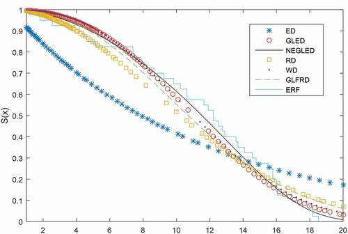
The log-likelihood value of NEGLED model is largest compare to the considered models which indicates the best fit of NEGLED to the given dataset, see Table 5. At 5% significance level the ${\chi }_{0.05}^2$ critical values for 1, 2, 3, and 4 d.f. are 3.841, 5.991, 7.815, and 9.488, respectively. Next, the LR test statistic for all the models are greater than ${\chi }_{0.05}^2$ critical values for corresponding d.f., see Table 5. Consequently, at 5% level of significance, we reject all the null hypotheses i.e. GLFRD, GLED, RD, WD, and ED. Considering all the above results, we may conclude that the NEGLED model is superior competitor for lifetime datasets than the ED, RD, WD, GLFRD, and GLED models.

6. Conclusion

In this article, a new distribution named NEGLED has been introduced which generalizes the GLED model studied by Mahmoud and Alam (2010) and several other well-known distributions. We investigated some statistical properties of the proposed distribution like HRF, quantile function, random sample generation, moments, stress–strength parameter, and order relations. To illustrate the MLEs behavior with increasing sample size, MLE and inference for the NEGLED model using simulation were obtained. It was found that the MLE method provides good estimates for the NEGLED model. At last, using the proposed distribution and some well-known distributions, a real-life dataset is fitted. It was found that, compared to the other distributions (ED, RD, WD, GLED, and GLFRD), the NEGLED model offers a better fit to the Leukemia dataset. Therefore, accounting the flexibility of PDF and HRF, the NEGLED model can be utilized as an effective model for lifetime data applications.

Acknowledgements

We are very thankful to the Editorial board and the reviewers for their valuable comments and suggestions which helped to improve the manuscript significantly.

Disclosure statement

No potential conflict of interest was reported by the authors.

Additional information

Funding

This work was supported by the No direct funding.

Notes on contributors

Neeraj Poonia

Neeraj Poonia obtained his M.Sc. in Statistics (2017) from the Central University of Punjab, Bathinda, India. He is currently pursuing his Ph.D. in Statistics in the School of Basic Sciences at the Indian Institute of Technology Mandi, Himachal Pradesh, India. His research interest includes probability distribution theory and applied statistics.

Sarita Azad

Sarita Azad obtained her Ph.D. in Mathematics (2008) from Delhi University and the Indian Institute of Science, India. She is currently working as an assistant professor in the School of Basic Sciences at the Indian Institute of Technology Mandi, Himachal Pradesh, India. Her area of research includes climate change modelling, statistical data analysis, time series analysis and forecasting, and distribution theory.