Agricultural eco-efficiency and climate determinants: application of dea with bootstrap methods in the tropical montane cloud forests of Puebla, Mexico

ABSTRACT

This research analyzes the eco-efficiency of peasant production in a sample of 32 Puebla municipalities located in the tropical montane cloud forests (TMCF) and the influence of climatic factors, considering data from two years 2016–2017. Therefore, window data envelopment analysis approach with bootstrap in two stages was used. The results allow us to draw two basic conclusions. 1) It is possible, imitating the benchmarks, at the aggregate level in the region, to increase annual revenue and preserved areas by 58.7%, with the same inputs; or equivalently, reduce inputs and environmental costs by 36.98% with the same level of production. 2) Eco-efficiency scores are significantly affected by climatic factors and thus, the increase in temperature and the reduction in precipitation should have predominantly positive impacts on the region’s eco-efficiency. This finding should be based on the characteristics of the region—humid mountainous forest with rain for most of the year and persistent mist almost at ground level. Based on this information, strategies can be defined by decision makers to harmonize economic growth and environmental preservation, as well as adaptive policies and actions to reduce vulnerability and improve the resilience of peasant producers.

KEYWORDS:

• eco-efficiency
• farming
• Tropical Montane Cloud Forests
• Climate Determinants
• DEA with two-stage bootstrap

1. Introduction

One of the themes discussed at the 26th United Nations Conference on Climate Change in Glasgow, Scotland, was the preservation of forests. At this conference, according to the website (https://news.un.org/en/story/2021/11/1104642), 110 countries, home to 85% of the world’s forests, signed a declaration, pledging to stop and reverse deforestation by 2030. This is an important step; however, the next and most difficult is the implementation of this commitment at the regional and local level, without compromising the sustainable development of the communities that live there.

In many forests, a large number of economically vulnerable small farmers live and work. They are families with limited resources to maintain or increase productivity and competitiveness, marginalized from social assistance, and affected by the fragmentation of rural properties with the independence of their adult sons (Donatti et al., 2019). Therefore, the implementation of increasingly strict regulations on environmental protection has generated a notable concern about its effects, a priori, negative in these communities.

This situation is no different in Mexican tropical montane cloud forests (TMCF),¹ where decision-makers face two major challenges. The first indicates the need to make the communities that live there more productive and efficient so that they can offer more products with higher quality and competitive prices, capable of facing the direct competition of industrial-scale agriculture (Morton, 2007). The second challenge arises from the evidence that agricultural intensification and expansion in forestry areas can generate environmental damage not offset by economic benefits. The removal of native primary vegetation cover compromises the ecosystem services provided by flora and fauna, which also run the risk of degradation. It induces erosion, a reduction in soil nutrients, and an increase in greenhouse gas (GHG) emissions, which end up interfering with both the rainfall regime and the planet’s temperature. This creates a vicious cycle, as changes in temperature and precipitation patterns can damage the agricultural activity itself (Donatti et al., 2019; Kummu et al., 2021).

Therefore, the challenges in this region demand answers to the following questions: Is it possible to raise production and, at the same time, reduce environmental impacts and the use of production inputs? in other words, is a more eco-efficient agriculture feasible? If plausible, to what extent can agriculture be more eco-efficient in? How can temperature and precipitation affect eco-efficiency? Around these questions is the central problem of this article.

In recent decades, the literature has shown great contributions to the development of robust models for empirical analysis of efficiency, productivity, eco-efficiency, and their determining factors (Emrouznejad & Yang, 2018). From the seminal works of Simar (1992) and Wilson (1993), innovative approaches have emerged using bootstrap techniques to overcome the limitations of classical models: Stochastic Frontier Analysis—SFA (Aigner et al., 1977; Meeusen & van den Broeck, 1977) and Data Envelopment Analysis—DEA (Charnes, Cooper, & Rhodes, 1978). These approaches fall under the so-called stochastic and semiparametric DEA and make a symbiosis that integrates the random term contained in SFA-type methods to the boundary estimated by non-parametric DEA-type methods.

Although the use of the stochastic and semiparametric DEA model has become popular in the last decade, in the most diverse areas, there is a gap in the literature, especially in the study of the relationship between climatic factors and agricultural eco-efficiency. As far as is known, in the case of the analysis of Mexican agriculture with this method, there are no studies on eco-efficiency, and articles on the impact of climate factors on efficiency and productivity in Latin America and the Caribbean are scarce (Lachaud et al., 2017). Even so, it is possible to cite some works that include in the study of the efficiency and productivity of climatic variables: Mullen (2007) for the analysis of Australian agriculture; Villavicencio et al. (2013) for the USA; Khanal et al. (2018) for Nepal; Ojo and Baiyegunhi (2020) for Gori-Maia et al. (2021) for Brazil.

This study aims to estimate robust two-stage bootstrap DEA eco-efficiency scores for agriculture in TMCF of the State of Puebla, on a municipal basis, considering data from 2016–2017. For this, in the first stage, the classic inputs and products of the sector were used, adding two environmental externalities: one positive and the other negative. At this stage, bootstrap techniques allowed for detecting outliers, estimating bias, correcting scores, as well as testing the type of returns to scale and the evolution of eco-efficiency in the two years studied. In the second stage, temperature and precipitation variables are used to explain the corrected eco-efficiency using the truncated Tobit regression model.

In this way, the study provides insights into benchmarks, goals for improving eco-efficiency in low-performing municipalities, and the possible impact of climate variables. It is hoped that the results can be particularly useful for formulators and decision-makers in defining and designing strategies that harmonize economic growth and environmental preservation, supporting the region’s sustainable development.

2. Background

The TMCF represents a biome that occupies a small area of the planet’s surface. Bruijnzeel (2001) estimated that, at the beginning of the 21st century, these woods occupied around 381,000 km², approximately 0.26% of the planet’s area. Despite its small size, it is a biome that contributes a set of ecosystem services. This type of forest provides wood, food, medicinal substances and fibers, purifies and preserves water resources and conserves fauna and flora.

In Mexico, one area of TMCF is located at the Oriental Sierra Madre, in rugged terrain with an altitude ranging from 400 to more than 2,800 meters above sea level, with temperatures around 12 to 20 °C and high humidity due to frequent rainfall that range between 1000 and 3000 mm. In 2013, it was estimated that the area of the Mexican TMCF was almost 17,000 km² (1% of the national territory) and, despite being highly fragmented and dispersed, four-fifths were considered to be unchanged; the remaining was made up of almost 12% of the degraded area, 6% of the deforested area and 2% of area under-recovery (Sánchez-Ramos & Dirzo, 2014).

The Comisión National para el Conocimiento y Uso de la Biodiversidad (CONABIO) in its Information System on TMCF, reports the existence of great diversity: for example, 5533 species only with flowers, added to the 630 species of ferns and related plants. This represents 27% of the country’s floristic richness and about 2% of the world’s total floristic (Villaseñor, 2010). Nevertheless, given the fragility of the TMCF and the deterioration caused by human activities, there is a transition to an ecosystem that replaces primary vegetation with secondary vegetation, the fragmentation of the biome, and the migration and extinction of animals and plants (Cruz-Cárdenas et al., 2014). Families in the region practice shade coffee planting but carry out subsistence agriculture by cutting and burning the forest, which increases the degradation of the biome.

3 Theoretical methodological framework

In economics, efficiency develops from the joint concept of production possibility (CPP)—technology set (T). This set incorporates the transformed inputs (x) and the outputs (y) generated by a set of available production processes. It is expressed mathematically as:

(1) $T=\left\{\left(x,y\right)|xcanproducey\right\}$(1)

where: in a broader concept (eco-efficiency), vector x represents production factors and environmental costs; and y is the set of desired products, including positive externalities.

Shephard (1972) and Färe (1988) describe the properties of the CPP. These properties define a space in the negative as ${\mathrm{\Re }}^{p+q}$, constituted by the x and $\mathbf{y}\in {\mathrm{\Re }}^q$ of the n productive units (called DMUs—Decision Making Unit) that make up the CPP. The upper limit of space determines the boundary $\left(T^{\delta }\right)$ of the CPP that involves the points that represent the DMU. Farrell (1957) shows that it is possible to build this boundary with linear segments, from the convex combinations of efficient DMUs. Thus, inefficient DMUs are located in points inside the CPP, showing that they are not maximizing production or minimizing inputs.

Hence the concept and measures of eco-efficiency. Eco-efficiency is revealed when a DMU obtains the highest level of desired products possible with a given level of input and environmental impact or when it requires the least possible amount of inputs and environmental cost to produce a given number of products. Its measurement results from the calculation of the Euclidean distance that separates each DMU from the border formed by the benchmarks. Thus, it is possible to define two measures of technical efficiency (): i) Farrell’s technical efficiency-oriented to maximize outputs with a given input level, ${\theta }_{OO}$; ii) Farrell’s technical efficiency aimed at minimizing the inputs with a given level of products, ${\theta }_{IO}$. Farrell’s (1957) efficiencies are inverse to Shephard’s (1970) radial efficiencies.

3.1 DEA Models

Having a set of n CPP observations $\left(S_n=\left\{x_i,y_{i}toi=1,\dots ,n\right\}\right)$ it is possible to estimate the frontier of the CPP ($T^{\delta })$ and the Farrell efficiency $\theta$, using the Data Envelopment Analysis (DEA) method. This is a nonparametric linear programming procedure, developed by Charnes, Cooper & Rhodes (1978) and called the DEA-CCR or CRS model. It characterizes the technology through the estimator ${\hat{T}}_{CCR}$ of T and calculates $\hat{\theta }$, an estimator of $\theta$, imposing the properties of constant return to scale (CRS). The output-oriented eco-efficiency estimator with ${\hat{T}}_{CCR}$ e $\left(x_i,y_i\right)$ for each DMU_i is defined with the following linear programming problem (PPL):

(2) ${\hat{\theta }}_i{\left(x_i,y_i\right)}_{CCR-OO}=max\left\{{\hat{\theta }}_i|{\hat{\theta }}_i{y}_i\le Y\lambda ,x_i\ge X\lambda ,\lambda \in {\mathcal{R}}_{+}^n\right\}$(2)

where Y= [y₁, …,y_n] and X= [x₁, …,x_n] represent, respectively, the matrices of the outputs (including the positive externalities) and inputs (including the environmental costs) of the n observations; x_i e y_i—the vectors of inputs and outputs, respectively, of the assessed DMU_i; $\lambda$ =[$\lambda$ ₁, … $,\lambda$ _n] _1xn—the vector that determines the linear combination of the best practices in the construction of the frontier. ${\hat{\theta }}_i$ is the output-oriented eco-efficiency index of DMU_i that must be greater than or equal to 1. If ${\hat{\theta }}_i=1$ the DMU_i is considered eco-efficient. For other cases, it will be eco-inefficient. ${\hat{\theta }}_i{y}_i$ gives the projection of ($x_i,y_i)$ on the frontier, at the maximum level of outputs possible with the available inputs. In this way, it is possible to define improvement targets for eco-inefficient DMUs.

Similarly, one can define a new PPL and find the input-oriented eco-efficiency estimator for each DMU_i.

(3) ${\hat{\theta }}_i{\left(x_i,y_i\right)}_{CCR-IO}=min\left\{{\hat{\theta }}_i|y_i\le Y\lambda ,{\hat{\theta }}_i{x}_i\ge X\lambda ,\lambda \in {\mathcal{R}}_{+}^n\right\}$(3)

where $0<{\hat{\theta }}_i\le 1$. If ${\hat{\theta }}_i=1$ the DMU_i is considered eco-efficient. Otherwise, it will be eco-inefficient. ${\hat{\theta }}_i{x}_i$ determines the projection of ($x_i,y_i)$ on the efficient frontier and indicates the intensity of waste verified in the production process. It is necessary to register that with the technology with constant returns ${\hat{\theta }}_{i,CCR-IO}=1/{\hat{\theta }}_{i,CCR-OO}$.

The DEA-CCR model was further complemented by Banker et al. (1984) to include the property of increasing, constant, or decreasing scale income in different parts of the frontier. This is called the DEA-BCC or VRS model, in which the PPL for the product-oriented eco-efficiency estimator with ${\hat{T}}_{BCC}$ for each DMU_i is defined:

(4) ${\hat{\theta }}_i{\left(x_i,y_i\right)}_{BCC-OO}=max\left\{{\hat{\theta }}_i|{\hat{\theta }}_i{y}_i\le Y\lambda ,x_i\ge X\lambda ,1\lambda =1,\lambda \in {\mathcal{R}}_{+}^n\right\}$(4)

On the other hand, the PPL of the input-oriented DEA-BCC model is:

(5) ${\hat{\theta }}_i{\left(x_i,y_i\right)}_{BCC-IO}=min\left\{{\hat{\theta }}_i|y_i\le Y\lambda ,{\hat{\theta }}_i{x}_i\ge X\lambda ,1\lambda =1,\lambda \in {\mathcal{R}}_{+}^n\right\}$(5)

Thus, for a DMU_i, the ${\hat{\theta }}_{BCC}$ is estimated by adding, in the DEA-CCR PPL, the restriction $1\lambda =1$, that is, ${\sum }_{i=1}^n{\lambda }_i=1$. This allows incorporating the variable returns property and ensuring that DMU_s are only compared with DMU_s of equivalent size, disregarding scale inefficiency.

The explanation of the scores ${\hat{\theta }}_{BCC-OO}$ and ${\hat{\theta }}_{BCC-IO}$ is the same as in the DEA-CCR model, concerning the maximum possible level of outputs and the minimum possible level of inputs, respectively. However, ${\hat{\theta }}_{BCC-IO}\ne 1/{\hat{\theta }}_{BCC-OO}$ and the DEA-BCC efficiency will always be greater than or equal to that achieved with DEA-CCR, that is, the BCC efficiency scores tend to be less restrictive than those obtained with DEA-CCR.

Cooper et al. (2007) present other extensions of the DEA model. Among them, we are interested in the Window Analysis model. Window analysis, proposed by Charnes et al. (1984), is valid for measuring intertemporal efficiency. It allows analyzing the same DMU in several periods (t) and identifying the year in which the DMUs were more or less efficient. Therefore, the sample has n*t observations. This increases the number of DMUs analyzed, which can be useful when dealing with small samples. In addition, it is possible to use DEA with unbalanced panel data, that is, panels that do not have the same number of DMUs in each period. However, the DEA window analysis implicitly assumes that each DMU is independent, different in each period and that there are no technical changes in the analyzed period.

3.2 Outlier detection

The models specified above are deterministic, calculate punctual efficiency values, and thus become sensitive to measurement errors and omissions as well as to the existence of outliers. Therefore, its application requires a previous data cleaning procedure. Wilson (1993) suggests a first step, such as exploratory data analysis, before using any boundary estimation.

Bogetoft and Otto (2011) recommend the multivariate data cloud method to detect outliers. This method identifies the atypical cases by calculating the influence of each DMU on the CPP. The influence refers to the impact of removing one DMU from the sample on measuring the efficiency of other DMUs. The method starts by calculating the volume of the point cloud (in the space formed with the variables used), estimated by the determinant of the input-output matrix. Afterward, a DMU is removed and the volume change is observed. If the volume variation is high, then it is possible to conclude that said DMU is an outlier. The volume change is calculated by R⁽ⁱ⁾ = D_i/D, where D is the determinant of the initial matrix and the D_i—determinant after DMU_i removal. Therefore, if the DMU_i is not an outlier, R⁽ⁱ⁾ will have a value close to 1; otherwise, its value will be close to zero, denoting an influential observation.

The process must be repeated for each DMU and a growing set of deleted DMUs. The number (r) of removed DMUs in the pool is arbitrary at the researcher’s discretion. However, its size must be large enough to detect outliers masked by other outliers. Usually, 10% of the sample is taken, following the estimates of Banker and Chang (2006). When examining the values of R^r for the sets of r DMUs, we look for the first smallest value, which is compared with the other R^r. If the difference is large, the $R_{min}^r$ will be formed by a group of outliers. To get a clear picture of these differences and how they depend on the number of DMUs excluded Wilson (1993 and 2008) recommends building a graph with the ordered pairs $\left(r,log\left(R^r/R_{min}^r\right)\right)$. In this graph, outliers are identified when there is a relatively large interval between the points above 0 and the point at 0.

3.3 Statistical inference of bootstrapped DEA estimators

Another problem of classical DEA models, arising from their deterministic nature, is related to the estimation of point values without debating the stochastic noise and uncertainty surrounding this estimate. However, it would be of great relevance for empirical use if eco-efficiency analysis were complemented with statistical inference techniques that define confidence intervals, hypothesis testing, and correlation analysis. This allows for evidence of the reliability and acceptance of the scores of the DEA models and helps to qualify comparisons of eco-efficiency between DMUs, as well as the effect of exogenous variables. To make this complementation and obtain more robust efficiency indicators, a semi-parametric and stochastic DEA based on bootstrap techniques was developed.

The stochastic DEA is based on the fact that the set of n observations is just a sample of the CPP, which is not exhaustively known. Therefore, it is assumed that both the inputs and outputs and the eco-efficiency scores are random variables, resulting from an unknown data generating process (DGP), an underlying density function from which other observations can be produced. Naturally, it is assumed that there is a bias between the true technology T (unknown and unobservable) and the $\hat{T}$ estimated based on a given sample of observations.

For small samples with unknown distributions, bootstrap is the most appropriate method for statistical inference. Bootstrap is widely used to obtain estimates with greater precision, calculate bias, and confidence intervals and perform hypothesis tests on parameters of interest. The main idea of bootstrap is to obtain a “new” set of random data, resampled with replacement over the original data set (Efron & Tibshirani, 1993). Resampling is repeated several times to create new samples (pseudo-samples) of the same size as the original. From the set of samples, we obtain the distribution of the estimates of the parameter of interest which should be like the true one, and we can draw robust conclusions about the statistics that interest us. In other words, the essence of the bootstrap is to generate a fictitious distribution so like the real one that the results obtained from it can be considered analogous to those obtained with population data.

In this work, DEA based on bootstrap techniques will be used to estimate eco-efficiency confidence intervals and test three hypotheses: the existence of return to scale, the difference in eco-efficiency between two periods, and the dependence between eco-efficiency and external factors.

3.3.1 Bootstrap to estimate bias and confidence interval of DEA indexes

To operationalize this procedure, Simar and Wilson (1998) suggested a special type of bootstrap, called smooth. This is different from the classic naive bootstrap, which is inconsistent in inferring DEA indicators. In this new proposal, new bootstrap efficiency indexes for each DMU (${\hat{\theta }}_i^{\ast })$ are estimated from the initial indexes, using a kernel density estimate with smoothing and reflection methods. Then, these new indexes are used to generate a new sample $S_n^{\ast }$ formed (respecting the radial nature of the efficiency) as follows: to estimate ${\hat{\theta }}_i^{\ast }{\left(x_i^{\ast },y_i^{\ast }\right)}_{OO}$ use $y_i^{\ast }=y_i\frac{{\hat{\theta }}_i^{\ast }}{{\hat{\theta }}_i}$ and $x_i^{\ast }=x_i$; to estimate ${\hat{\theta }}_i^{\ast }{\left(x_i^{\ast },y_i^{\ast }\right)}_{IO}$ is given by $x_i^{\ast }=x_i\frac{{\hat{\theta }}_i}{{\hat{\theta }}_i^{\ast }}$ and $y_i^{\ast }=y_i$. With these new inputs and outputs, we get a new efficiency index ${\hat{\theta }}_i^{\ast }$. By replicating this process B times for each DMU we will have a vast amount of bootstrap efficiency scores, a set ${\left\{{\hat{\theta }}_i^b\right\}}_{b=1}^B$ and a joint density function $\hat{f}\left(x_i^{\ast },y_i^{\ast }\right)$ for each DMU_i. This distribution provides a reliable estimate of the true efficiency index of DMU_i, this reliability being greater when B → ∞ and n → ∞. Simar and Wilson (1998) suggest that at least 2000 samples are needed for asymptotic results to be good.

As Simar and Wilson (1998) point out, when the bootstrap is consistent, the distinction between initial efficiency (${\hat{\theta }}_i$) and bootstrap efficiency (${\hat{\theta }}_i^{\ast }$) should be similar to the difference between initial efficiency and true efficiency (${\theta }_i$) for a given DMU_i:

(6) $\left[{\hat{\theta }}_i^{\ast }-{\hat{\theta }}_i\right]\stackrel{aprox}{\to }\left[{\hat{\theta }}_i-{\theta }_i\right]$(6)

Therefore, the bias for each DMU_i can be revealed, by the equations:

(7) ${\widehat{bias}}_i=\frac{1}{B}\sum _{b=1}^B{\hat{\theta }}_i^{\ast }-{\hat{\theta }}_i={\overline{\stackrel{ˆ}{\theta }}}_i^{\ast }-{\hat{\theta }}_i$(7)

where ${\overline{\stackrel{ˆ}{\theta }}}_i^{\ast }$ is the average of B bootstrap efficiency estimates of the DMU_i. So, the estimator of $\theta i$ with bias correction is:

(8) ${\tilde{\theta }}_i={\widehat{\theta }}_i-{\widehat{v{i}^{\prime }es}}_i={\widehat{\theta }}^i-{\overline{\widehat{\theta }}}_i^{*}+{\widehat{\theta }}_i=2{\widehat{\theta }}_i-{\overline{\widehat{\theta }}}_i^{*}$(8)

It is also observed that knowing the empirical distribution of bootstrap efficiency and bias, it is possible to estimate confidence intervals with a significance level (1-α), computing the critical values a_α and b_α, so that

(9) $Pr\left[-b_{\alpha }\le {\hat{\theta }}_i^{\ast }-{\hat{\theta }}_i\le -a_{\alpha }\right]\approx Pr\left[-b_{\alpha }\le {\hat{\theta }}_i-{\theta }_i\le -a_{\alpha }\right]\approx 1-\alpha$(9)

To calculate a_α and Simar and Wilson (1998, 2000) propose the use of the percentile method, which is based on ordering bias-corrected estimates from highest to lowest and eliminating, at both ends of this ordering, the percentage (α/2) of values. Thus, the estimated confidence interval will be

(10) ${\hat{\theta }}_i+a_{\alpha }\le {\theta }_i\le {\hat{\theta }}_i+b_{\alpha }$(10)

This procedure, formulated for the DMU_i, is the same that must be followed for each and every one of the other DMUs that make up the original sample.

The smoothed bootstrap algorithm to estimate the bias and confidence interval of DEA indexes is operated by the R boot.sw98 function available in the FEAR library (Wilson, 2008).

3.3.2 Test of the return to scale model

The freedom to choose one model (CCR or BCC) or adopt multiple models may be inadequate. Taking an unproven assumption about frontier returns to scale can seriously change efficiency measures if the actual technology is another (Simar & Wilson, 2002). Therefore, in the development and validation of the DEA method, one must test whether the set of technology T from which our observations are sampled exhibits constant returns to scale or not. The authors formalize the test with a pair of hypotheses: the null hypothesis (H₀): T is CCR or the alternative hypothesis (H_a): T is BCC, using the following estimator:

(11) $S=\frac{{\sum }_{i=1}^n{\hat{\theta }}_{i,CCR}}{{\sum }_{i=1}^n{\hat{\theta }}_{i,BCC}}$(11)

where, S ≤1, since ${\hat{\theta }}_{i,BCC}\ge {\hat{\theta }}_{i,CCR}$. If S is close to 1, H₀ must not be rejected and if S is significantly less than 1, H_a must be considered true. Therefore, we must find a critical value $c_{\alpha }$ that will determine whether we should reject H₀, when S <$c_{\alpha }$ is according to a significance level: usually 5%.

The distribution of the population parameter of S is unknown. Therefore, it is not possible to determine $c_{\alpha }$ immediately. To estimate the distribution of this estimator, Simar and Wilson (2002) advise using the bootstrap technique. With the help of the R boot.sw98 function, the algorithm obtains the sets of bootstrap efficiency scores for the CCR model, for the BCC model, and the distribution of S. In this way, we can compare the estimated value of S in (11) with the critical value at 5% to decide on H₀.

3.3.3 Efficiency difference test for two periods

According to Bogetoft and Otto (2011), if the set of n DMUs is divided into two groups with K₁ and K₂, where n = K₁ + K₂, we may also be interested in testing whether there are significant differences between the efficiencies of the two groups. The authors argue that this procedure is relevant if one intends to test whether a specific treatment in a group of DMUs is more efficient than another, whether a specific region offers more favorable conditions for companies than another, etc. In our case, we are interested in testing whether the distribution of eco-efficiency of municipalities in 2016 ($\hat{f}\left({\theta }_{2016}\right))$ is significantly different from 2017. Thus, the test can be formalized as the null hypothesis, H₀: $\hat{f}\left({\theta }_{2016}\right)$= $\hat{f}\left({\theta }_{2017}\right)$; versus the alternative hypothesis, H_a: $\hat{f}\left({\theta }_{2016}\right)\ne \hat{f}\left({\theta }_{2017}\right)$.

There are several ways to perform these tests. If the assumption of the efficiency distribution is not possible, Banker (1993) suggests using the Kolmogorov-Smirnov (K-S) test and Bogetoft and Otto () complement it with the Kruskal-Wallis test. Thus, these tests will be used to verify the equality of the two corrected eco-efficiencies distributions.

3.3.4 Testing the dependence of eco-efficiency on external factors: Second-stage analysis

After estimating the corrected indexes and performing the aforementioned tests, for Bogetoft and Otto () naturally the following questions arise: why are some DMUs more efficient than others? Is efficiency affected by weather disturbances and other exogenous factors?

The search for answers to these questions led to the emergence of the semi-parametric technique called two-stage analysis (Simar & Wilson, 2007). In the first, the corrected efficiency indexes are calculated and, in the second, we try to identify the impact of other variables (Z) on the efficiency of the DMUs. These variables (Z) are called exogenous, non-discretionary variables and can be internal or external to the production process. Lovell (1993) advises the use of variables under the manager’s control in the first stage and variables over which the producer does not control in the second, such that the second stage variables are not correlated with the inputs and outputs used in the first.

To investigate whether a Z vector explains variations in efficiency, Tobit regression is usually used. This method is estimated by maximum likelihood and is used when the dependent variable is truncated by value ranges. However, as the DEA efficiency indexes have serial correlation and there is often multicollinearity in the contextual variables, biased results can be obtained, especially when the sample is small.

To overcome this problem, Simar and Wilson (2007) indicate the application of bootstrap to a truncated regression model (Tobit or equivalent) in which $\theta i=Z_i\beta +{\epsilon }_i$. Here, $\theta i$ represents the corrected eco-efficiency, estimated in the first stage; $Z_i$ is the vector of predictor variables that are expected to explain the eco-efficiency indices through the vector of parameters $\beta$ to be estimated; and the vector ${\epsilon }_i$ is the random error associated with each DMU, indicating the part of eco-inefficiency not influenced by $Z_i$. It is assumed that ${\epsilon }_i$ has a normal distribution with an average 0 and variance ${\sigma }_{\epsilon }^2$ censored between 0 and 1. This procedure allows you to test consistently which are the significant influencing variables and their sign (positive or negative).

Simar and Wilson (2007) developed two algorithms that incorporate the bootstrap procedure into a truncated regression model. In this research, we will use Algorithm #1, recommended for samples with less than 400 units and up to three outputs and three inputs.

4 Variables

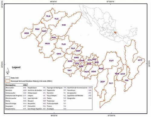
This section describes the sample and data used. The sample consisted of a group of 32 municipalities in the State of Puebla (Figure 1), representing 15% of the 217 municipalities in this State. They are located in the TMCF, in the mountainous region of Sierra Norte, east of the capital of the Mexican Republic and have a humid and hot climate, with abundant rainfall in summer. Families practice planting coffee in the shade and do subsistence agriculture by cutting and burning the forest, which increases the degradation of the biome.

Figure 1. Municipalities of Puebla, located in the TMCF.

The analysis of these municipalities was carried out in terms of input and output indicators commonly used for agricultural efficiency and productivity analyses. But a negative externality was added as input and a positive environmental externality as an output. More specifically, the following variables were considered. As input: x₁—people employed in the primary sector (paid and familiar); x₂—an area of agricultural use in hectares; x₃—greenhouse gas (GHG) emissions in the agricultural sector in tons of CO₂ equivalent which represents a proxy of the environmental cost; as outputs: y₁- total production value in thousands of Mexican pesos; y₂- a preserved area with forest in hectares, which represents a proxy of environmental services provided by nature in this area.

Furthermore, to investigate the association of climatic factors with eco-efficiency in the second stage, the average annual temperature (in °C), precipitation of the municipalities (in mm) and their squared values (T^2 and P^2) were selected. The inclusion of T^2 and P^2 is because at the extremes of these variables (low or high temperatures and lack or excess of precipitation) we must observe similar effects and their impacts are not constant (that is, they have different rates of variation -ascending or descending).

Data were extracted to two years (2016 and 2017) from different official databases according to Hernández Cayetano (2020) (See end of text “Data Availability Statement” section).

5 Results analysis

5.1 Descriptive analysis, outlier detection, and final sample

Table 1 shows the descriptive statistics of inputs, products, and climate variables, allowing for an overall view of the sample referring to the 64 DMUs analyzed (32 municipalities in 2 years −2016-2017). The Table indicates that, for all variables, the minimum values are well below the 1st quartile and the maximum values are well above the 3rd quartile. This shows the existence of significant heterogeneity in the data and evidence of potential extreme observations (outliers), mainly in y₁- total production value.

Table 1. Descriptive statistics of inputs (x), outputs (y), and environmental determinants

	x1	x2	x3	y1	y2	T	P
Average	2124.44	5667.62	332.98	47171578.94	2694.39	17.10	2316
Median	1545.00	3747.17	250.00	17190019.53	2499.48	16.96	2234
Standard deviation	1702.94	5011.00	284.70	76477785.67	2107.35	1.548	565.8
Minimum	50.00	109.95	86.00	359510.05	60.55	14.43	1212
1st quartile	851.80	1578.60	167.50	9294241.00	1253.19	15.99	1977
3rd quartile	3073.50	8649.20	356.00	60205400.00	3418.06	18.14	2610
Maximum	6078.00	22458.00	1421.00	505135644.70	8787.10	21.89	4098

As pointed out, DEA models are especially sensitive to the presence of outliers. Therefore, a preliminary purification of the data was performed, using the routine developed by Wilson (1993) in the FEAR 2.01 package for the R programming language. In this analysis, the possibility of removing more than 10% of the sample was considered, an r =8, an acceptable size for a sample 64.

The results are presented in Table 2, which show which exclusions provide the minimum value of R^r (the ratio of the new volume of the data cloud to the initial volume). The first line of Table 2 shows that the exclusion of DMU 45 will result in a value of R¹ =0.2015, the minimum value of R¹ when only one observation is excluded from the sample. The second line, r =2, indicates that excluding DMUs 54 and 45 simultaneously we obtain an R² =0.1335. The same understanding is valid for the other lines. Complementing the Table, Graph 1 represents a dashed line connecting the second lowest values for each r, illustrating the separation between the lowest log ratios for each r value. Thus, for r = 1 a jump relatively larger than the rest is obtained when excluding the DMU₄₅, the Tlatlauquitepec municipality of 2016 (TLT16).

Table 2. Matrix of outliers for the initial sample

r	Deleted observations	${\mathrm{R}}_{min}^{\left(\mathrm{r}\right)}$
1	45	0.2015
2	54 45	0.1353
3	53 54 45	0.0772
4	23,535,445	0.0517
5	2,324,535,445	0.0266
6	232,453,185,445	0.0174
7	23,245,318,175,445	0.0095
8	2,324,555,318,175,445	0.0063

Analyzing the TLT16 municipality, it is possible to notice the existence of a possible typographical error in the variable y₁- total production value. This value is the maximum observed in Table 1, being 10 times greater than y₁ for this municipality in 2017. Therefore, it was decided to remove this DMU from the sample.

Graph 1. Log-ratio for the initial sample.

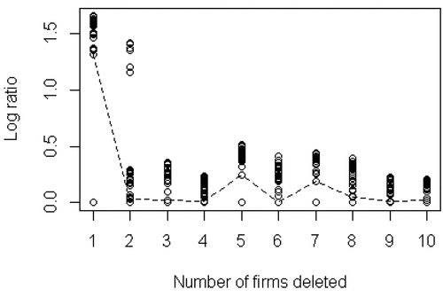
In Graph 1, we observe two other jumps: r =5 and r =7. However, the DMUs that form r =5 and r =7 (except 45) are neither at the minimum input extremes nor at the maximum output extremes. Therefore, because they are relatively smaller jumps, it was decided to keep these DMUs in the sample. Decisions about atypical cases are not mechanical, they must be taken with prudence. Simar and Wilson (2015) indicate that determining what constitutes an outlier necessarily implies a certain subjectivity on the part of the researcher.

5.2 Statistical inference of DEA eco-efficiency

After defining the new sample (63 DMUs), the return to scale test was performed, since the choice of technology is a fundamental issue and if decided arbitrarily, inadequate conclusions can be reached. As already suggested, this test was performed using the CCR and BCC ecoefficiency scores with the DEA window analysis method and the bootstrap procedure. The null hypothesis of CRS technology prevalence can be rejected if the estimated statistic S in (11) is less than the critical value obtained by the bootstrap estimators.

Bootstrapping the test used 2000 replications, giving an S = 0.8157 and a critical value of 0.6541 at a 5% significance level. Thus, it is suggested not to reject the CRS technology. Therefore, it can be assumed that in the studied region the DMUs operate with a similar production scale, with no relative scale inefficiency.

This result must be supported by the geography of the region and by the fact that in the municipalities studied, peasants’ production oriented in part to subsistence economy predominates. In this type of mountain farming, production is carried out on small properties, with little technological diversity, low use of inputs and machines, and an insignificant amount of external labor, where the family usually plays the role of owner, manager and is still responsible for all production and marketing logistics. Without cooperatives, and technical and financial assistance, it is difficult to find significant inequality in the scale of production.

Adopting the CRS technology as the dominant one, we started to estimate the eco-efficiency values, considering the random error inherent in the data. Here, the window analysis and the DEA-Bootstrap proposal by Simar and Wilson (1998, 2000) was also used, using 2000 replications. As a result, a stochastic production frontier closer to the real one is established to estimate the eco-efficiency levels.

Graph 2 shows the bias-corrected efficiency estimates and 95% confidence intervals and Table 3 records the values of the main results: the deterministic and bias-corrected eco-efficiency levels and their confidence interval for the output-oriented CCR model. But, due to the large number of DMUs, only the three most eco-efficient and the three most eco-inefficient municipalities are shown in the Table. Thus, when closer to one (1) the DMU is more eco-efficient; otherwise, if eco-efficiency is greater than 1, it will be more eco-inefficient. The results confirm that there are non-negligible eco-inefficient behaviors in the region and, therefore, it is possible to increase eco-efficiency.

Graph 2. Bias-corrected efficiency estimates and 95% confidence intervals (Source: elaborated by the authors).

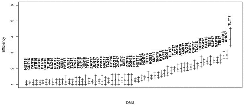
Table 3. Eco-efficiency

Dmu	Eco-efficiency without bias correction	Eco-efficiency with bias correction	95% confidence interval
			Lower limit	Upper limit
HUT16	2.028	1.094	1.009	1.207
CUT16	1.039	1.097	1.028	1.206
YAN16	1.000	1.114	1.009	1.264
. . .
AHC16	3.091	2.789	2.624	3.090
AHC17	2.942	2.830	2.644	3.128
TLT17	3.525	3.833	3.433	4.548
AVERAGE (STANDARD DEVIATION)	2.40 (2.44)	1.59 (0.58)	1.44 (0.46)	1.82 (0.64)

Source: Elaborated by the authors.

In Table 3, as in Graph 2, the DMUs were classified from lowest to highest corrected eco-inefficiency. It is noted that the DMU₁₅, the municipality Huitzilan de Serdán in 2016 (HUT16), was the best position in the ranking. Thus, the multiplication of its index by the product vector ($1.094\ast y_{15})$ will give the projection of this municipality on the efficient frontier, the maximum level of outputs with the available inputs (x₁₅). The municipality with the lowest eco-efficiency was Tlalauquitepec in 2017 (TLT17) with an index of 3.833, within the confidence interval 3,433–4.548. This allows us to consider that in this municipality, as well as in others that have very high scores, increasing its products to be eco-efficient will require a great effort. In this way, it is possible to define improvement goals for the evaluated municipalities.

From the results reported in Table 3, other important inferences are derived. The average of the bias-corrected indices was 1,587, indicating that in the region, on average, the total value of production and the preserved area with forest can increase by 58.7%, maintaining the level of inputs and emission of effect gases greenhouse—GHG. Equivalently, this index shows that it is possible to reduce inputs and emissions by 36.98% (1-(1/1.587)) with the same level of production. It is also observed that the mean and the standard deviation (0.58) of the corrected eco-efficiency levels is smaller than those obtained for the uncorrected eco-efficiency. In other words, the corrected eco-efficiency indices are more robust than the indices estimated by the deterministic DEA method, suggesting an overestimation of the latter. This finding highlights the relevance of performing the bootstrap analysis when estimating the efficiency indices in small samples. It also indicates that great caution should be exercised when performing comparative analysis between DMUs, since, as shown by the confidence interval, there may be no significant difference between the indices. If two intervals intersect, it would be possible to affirm that the units do not have statistically different levels of eco-efficiency.

Using the corrected indices, we continued with the tests on the difference in eco-efficiency of municipalities between 2016 and 2017. Table 4 presents the results of descriptive statistics and hypothesis tests on equality of distributions for the two groups, 2016 and 2017. Both the Kolmogorov-Smirnov and the Kruskal-Wallis tests estimated a p-value greater than the 0.05 significance level, which leads us not to reject the null hypothesis. In other words, the difference between the 2016 and 2017 eco-efficiency distributions is not significant. This conclusion is corroborated by the descriptive statistics of the two groups and by Graph 3, which represents the distributions, in box-plot format, of the eco-efficiencies of each group. This result must be supported by the low probability of significant changes in eco-efficiency from one year to another, where producers have low resources for investments.

Graph 3. Boxplot of the corrected eco-efficiency indexes for the groups (Source: elaborated by the authors).

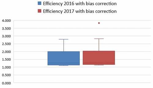
Table 4. Corrected eco-efficiency statistics for the Kolmogorov-Smirnov and Kruskal-Wallis groups and tests

	Group 1—municipalities 2016	Group 2—municipalities 2017
Minimum	1.094	1.134
1st Q.	1.131	1.173
Median	1.259	1.259
Average	1.546	1.627
3rd Q.	1.981	1.984
Maximum	2.789	3.833

Two-sample Kolmogorov-Smirnov test: d = 0.29032, p-value = 0.1151Kruskal-Wallis chi-squared test = 1.1207, df = 1, p-value = 0.2898Source: Elaborated by the authors

5.3 Impact of climate variations on eco-inefficiency indices

Figures 2 and 3 offer an overview of the temperature and precipitation levels, as well as the eco-efficiency indices calculated for the two years studied (2016 and 2017), respectively. The Figures do not allow us to visualize a clear pattern of correlation between climatic variables and eco-efficiency. Therefore, to understand the impact of climate on eco-efficiency, a Tobit regression analysis with bootstrap was performed between the corrected eco-efficiency (dependent variable) and the explanatory variables, temperature (T) and precipitation (P), considering their squared values (T^2 and P^2). With the four explanatory variables, the second stage model (Algorithm #1) by Simar and Wilson (2007, 2011) with 2000 replications is appropriate for an improvement in the statistical inference capacity of the relationship. In the application, output-oriented eco-inefficiency is the dependent variable that must be greater than or equal to 1. Therefore, it is necessary to clarify that a negative sign indicates a positive effect on efficiency (decreases eco-inefficiency) and a positive sign indicates a worsening (increases eco-inefficiency). Table 5 presents the results of the estimated model.

Figure 2. Temperature, precipitation, and eco-efficiency of 2016 in the study area.

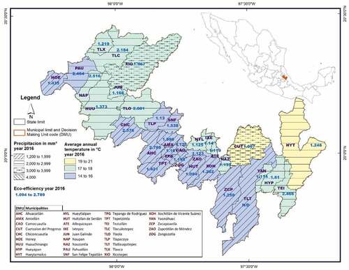
Figure 3. Temperature, precipitation, and eco-efficiency of 2017 in the study area.

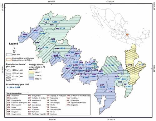
Table 5. Second stage model estimates

Model	Coefficient	95% confidence interval
		Lower limit	Upper limit
Intercepto	−36.4667100	−38.27547000	−34.65794000
T	4.9515190	4.72098800	5.18204900
P	−0.0014957	−0.00165565	−0.00133573
T^2	−0.1497322	−0.15647300	−0.1429913
P^2	0.0000005	0.00000043	0.0000005
Error deviation	1.4469570	1.44072400	1.45319000

Average marginal effect of temperature = −0.1610705Average Marginal Effect of Precipitation = 0.00065Source: Elaborated by the authors

The results reveal that both temperature and precipitation coefficients are statistically significant, at the 5% level, but they have a different impact on the eco-efficiency of the studied municipalities. As the estimated coefficients of the Tobit model cannot be interpreted as if they were linear regression estimators, the mean marginal effects were calculated, considering the two coefficients of both variables (T and P). The average marginal effect of temperature results in −0.1610705, which indicates that increasing the temperature by one unit reduces the eco-inefficiency by that value on average. Therefore, the increase in temperature contributes to improving eco-efficiency. The average marginal effect of precipitation was 0.00065, which indicates that reduction of the precipitation by one unit increases the eco-inefficiency in this value on average. Therefore, it is observed that the partial effect of temperature variability is greater than that of precipitation, which is very small.

The positive effects of increased temperature and reduced precipitation on eco-efficiency should be based on the characteristics of the region—humid mountain forest with rain for most of the year and persistent mist almost at ground level. In addition, it is known that these effects would reduce excess humidity, that creates an ideal environment for fungal proliferation, as well as promote restrictions on gas exchange in the soil, causing O₂ shortages and excess CO₂, impairing root development and biological nitrogen fixation in crops such as coffee and corn”.

6 Final considerations

In this work, agricultural eco-efficiency was estimated using the window data envelopment analysis approach in the municipalities of Puebla located in TMCF, pointing out how much it is possible to maximize economic and environmental objectives, having as reference the best practices of the region in 2016 and 2017. We employed the multivariate data cloud method, to identify and eliminate outliers that affect the eco-efficiency indices. Then, using bootstrap techniques, the scale-return significance test was performed. Once the CRS technology was confirmed, the corrected score for the random bias inherent in the data was estimated, as well as testing the difference in the eco-efficiency of the municipalities between 2016 and 2017. Furthermore, as the estimated scores are affected by uncontrollable factors not considered in the eco-efficiency calculations, truncated Tobit regression models with bootstrap were used to investigate how these environmental variables influenced these scores. In this way, an important gap is filled concerning the assessment of the environmental and economic performance of agriculture in one of the most vulnerable biomes in Mexico.

The results indicate that there are marked eco-inefficient behaviors. It is possible, at an aggregate level across the studied area, to increase annual agricultural revenue and preserved areas by 58.7%, with the same inputs and environmental costs, or equivalently, to reduce inputs and GHG emissions by 36.98% with the same level of annual agricultural revenue and preserved areas. Thus, the first and second questions of this research are answered, and it is shown that the results provide decision makers with important practical contributions to define policies that support the harmonization of economic growth and environmental preservation, as well as adaptive actions to reduce vulnerability and improve the resilience of peasant producers in the TMCF area in the face of possible climate changes.

The regression results answer the third question of this research and indicated that the eco-efficiency scores are also significantly affected by climatic factors. The results show that changes manifested by reduced rainfall and increased temperature will have predominantly positive impacts on the region. This must be explained by the mountainous and humid characteristics of the TMCF area.

The finding seems to dispute the general conclusions found in other research. For example, in the work of Sagarpa (2012) it is concluded that, in the region of the State of Puebla, the increase in temperature is related to a decrease in crop yields due to the stress caused by heat, the increase in fire. On the other hand, the reduction in rainfall has negative effects on productivity due to the incapacity of cultivation due to the lack of humidity, and dehydration of weeds and animals, among others. However, many of these researches are carried out considering extensive territories, warmer and more heterogeneous, disregarding the fact that the effects of climatic variations can be uneven in different regions. Hence, the importance of strengthening the studies in more homogeneous local scenarios that allow knowing the short-, medium- and long-term climate vulnerabilities to direct sustainable actions from the present.

Finally, it is necessary to emphasize that within the limitations of the study, one can consider the difficulty in obtaining disaggregated information to determine inputs, outputs, climatic data and to build a model with longer panel data. In this sense, as a line of future investigation, models are recommended that allow for the inclusion of trends in climate change, as well as contextual variables related to indicators of social, regional, and economic development.

Acknowledgements

The authors acknowledge the sponsorships from Consejo Nacional de Ciencia y Tecnología CONACYT(México); Secretaría de Investigación y Posgrado (SIP), IPN, México with the Project No. SIP20181987 and CIIEMAD- IPN are highly appreciated.

Disclosure statement

No potential conflict of interest was reported by the author(s).

Data Availability Statement

The database used and the data sources can be found in the open access link located in: https://data.mendeley.com/datasets/gf6xnkb5tw/1 and doi:10.17632/gf6xnkb5tw.1.

Additional information

Funding

This work was supported by the Consejo Nacional de Ciencia y Tecnología, CONACYT for Research Fellowship (SNI) of Mario del Roble Pensado-Leglise and Scholarship of Marisol Hernández Cayetano [Level II]; Instituto Politécnico Nacional, Proy SIP 20181987 [20181987; Consejo Nacional de Ciencia y Tecnología, CONACYT for Research Fellowship (SNI) of Mario del Roble Pensado-Leglise and Scholarship of Marisol Hernández CayetanoConsejo Nacional de Ciencia y Tecnología, CONACYT for Research Fellowship (SNI) of Mario del Roble Pensado-Leglise and Scholarship of Marisol Hernández Cayetano [Level II];

Notes

1. In this case, the notion of mesophilic mountain woods is considered equivalent to the notion of Tropical Montane Cloud Forests.

References

- Aigner, D., Lovell, C. A., & Schmidt, P. (1977). Formation and estimation of stochastic frontier production function models. Journal of Econometrics, 6(1), 21–14. https://doi.org/10.1016/0304-4076(77)90052-5
- Banker, R. D. (1993, October). Maximum likelihood, consistency and data envelopment analysis: A Statistical foundation. Management Science, 39 (10), 1265–1273. https://doi.org/10.1287/mnsc.39.10.1265
- Banker, R., & Chang, H. (2006). The super-efficiency procedure for outlier identification, not for ranking efficient units. European Journal of Operational Research, 175, 1311–1320. Ed. Elsevier. https://doi.org/10.1016/j.ejor.2005.06.028
- Banker, R. D., Charnes, A., & Cooper, W. W. (1984). Some models for estimating technical and scale inefficiencies in data envelopment analysis. Management Science, 30(9), 1078–1092. https://doi.org/10.1287/mnsc.30.9.1078
- Bogetoft, P., & Otto, L. (2011) Benchmarking with DEA, SFA, and . Ed. . ISSN pp. 0884–8289. Springer. ISBN 978-1-4419-7960-5 e-ISBN 978-1-4419-7961-2. https://doi.org/10.1007/978-1-4419-7961-2
- Bruijnzeel, L. A. (2001). Hydrology of tropical montane cloud forests: A reassessment. Land Use and Water Resources Research, 1(1732–2016–140258), 1.
- Charnes, A., Clark, C., Cooper, W., & Golany, B. (1984). A developmental study of data envelopment analysis in measuring the efficiency of maintenance units in the U.S. air forces. Annals Of Operations Research, 2(1), 95–112. https://doi.org/10.1007/BF01874734
- Charnes, A., Cooper, W., & Rhodes, E. (1978, Nov). Measuring the efficency of decision making units. European Journal of Operational Research, 2(6), 429–444. https://doi.org/10.1016/0377-2217(78)90138-8
- Cooper, W. W., Seiford, L. M., & Tone, K. (2007). Data envelopment analysis: A comprehensive text with models, applications, references and DEA-solver software (Vol. 2). Springer.
- Cruz-Cárdenas, G., Villaseñor, J. L., López-Mata, L., Martínez-Meyer, E., & Ortiz, E. (2014). Selección de predictores ambientales para el modelado de la distribución de especies en Maxent. Revista Chapingo. Serie ciencias forestales y del ambiente, 20(2), 187–201. https://doi.org/10.5154/r.rchscfa.2013.09.034
- Donatti, C. I., Harvey, C. A., Martinez-Rodriguez, M. R., Vignola, R., & Rodriguez, C. M. (2019). Vulnerability of smallholder farmers to climate change in central America and Mexico: Current knowledge and research gaps. Climate and Development, 11(3), 264–286. https://doi.org/10.1080/17565529.2018.1442796
- Efron, B., & Tibshirani, R. J. (1993). An introduction to the bootstrap (pp. 473). Chapman and Hall.
- Emrouznejad, A., & Yang, G.-L. (2018). A survey and analysis of the first 40 years of scholarly literature in DEA: 1978–2016. Socio-economic Planning Sciences, 61, 4–8. https://doi.org/10.1016/j.seps.2017.01.008
- Färe, R. (1988). Fundamentals of production theory. Springer-Verlag.
- Farrell, M. J. (1957). The measurement of productive efficiency. Journal of the Royal Statistical Society. Series A (General), 120(3), 253–281. https://doi.org/10.2307/2343100
- Gori-Maia, A., Silveira, R., Veneo, C., Burney, J., & Cesano, D. (2021). Climate resilience programmes and technical efficiency: Evidence from the smallholder dairy farmers in the Brazilian semi-arid region. Rev. Climate and Development. https://doi.org/10.1080/17565529.2021.1904812
- HernándezCayetano, M. (2020). Correlación espacial de ecoeficiencia y clima en los municipios poblanos del Bosque Mesófilo de Montaña de México. Tesis de Maestría, MCEAS-CIIEMAD-IPN, 27 de octubre de 2020. INSTITUTO POLITÉCNICO NACIONAL - CIIEMAD. https://tesis.ipn.mx/jspui/handle/123456789/29409
- Khanal, U., Wilson, C., Hoang, V.-N., & Lee, B. (2018). Farmers‘ Adaptation to Climate Change, Its Determinants and Impacts on Rice Yield in Nepal. Ecological Economics, Elsevier, 144(C), 139–147. https://doi.org/10.1016/j.ecolecon.2017.08.006
- Kummu, M., Heino, M., Taka, M., Varis, O., & Viviroli, D. (2021). Climate change risks pushing one-third of global food production outside the safe climatic space. Rev. One Earth, 4(5), 720–729. https://doi.org/10.1016/j.oneear.2021.04.017
- Lachaud, M., Bravo-Ureta, B., & Ludena, C. (2017). Agricultural productivity in Latin America and the Caribbean in the presence of unobserved heterogeneity and climatic effects. Rev. Climatic Change, 143(3–4), 445–460. http://dx.doi.org/10.1007/s10584-017-2013-1
- Lovell, C. K. (1993). Production Frontiers and Productive Efficiency. In H. O. Fried, C. K. Lovell, & S. S. Schmidt (Eds.), The measurement of productive efficiency-techniques and applications (pp. 3–67). Oxford University Press.
- Meeusen, W., & van den Broeck, J. (1977). Efficiency Estimation from Cobb-Douglas Production Functions with Composed Error. Published Wiley, Rev. International Economic Review, 18(2), 435–444. https://doi.org/10.2307/2525757
- Morton, J. (2007). The impact of climate change on smallholder and subsistence agriculture. Proceedings of the National Academy of Sciences, 104(50), 19680–19685. December 11, 2007 https://doi.org/10.1073/pnas.0701855104
- Mullen, J. (2007). Productivity growth and the returns from public investment in R&D in Australian broadacre agriculture. The Australian Journal of Agricultural and Resource Economics, 51(4), 359–384. https://doi.org/10.1111/j.1467-8489.2007.00392.x
- Ojo, T., & Baiyegunhi, L. (2020). Determinants of climate change adaptation strategies and its impact on the net farm income of rice farmers in south-west Nigeria. Rev. Land Use Policy, 95(1). https://doi.org/10.1016/j.landusepol.2019.04.007
- Sagarpa. (2012). México: El sector agropecuario ante el desafío del cambio climático. México: Secretaría de Agricultura, Ganadería, Desarrollo Rural, Pesca y Alimentación. http://www.sagarpa.gob.mx/programas2/evaluacionesExternas/Lists/Otros%20Estudios/Attachments/37/Cambio%20Climatico.pdf
- Sánchez-Ramos, G., & Dirzo, R. (2014). El bosque mesófilo de montaña: Un ecosistema prioritario amenazado. In Gual-Díaz, M. y A. Rendón-Correa (comps.). Bosques Mesófilos de Montaña de México: Diversidad, Ecología y Manejo (pp. 109–139). 978-607-8328-07-9. Comisión Nacional para el Conocimiento y Uso de la Biodiversidad. https://www.academia.edu/12475725/Bosque_Mes%C3%B3filos_de_Monta%C3%B1a_de_M%C3%A9xico_diversidad_ecolog%C3%ADa_y_manejo
- Shephard, R. W. (1970). The Theory of Cost and Production Functions. Princeton University Press.
- Shephard, R. W. (1971). Theory of Cost and Production Functions. Ed. Princeton University Press.
- Simar, L. (1992). Estimating efficiencies from frontier models with panel data: A comparison of parametric, non-parametric and semi-parametric methods with bootstrapping. Journal of Productivity Analysis, 3(1–2), 167–203. https://doi.org/10.1007/978-94-017-1923-0_11
- Simar, L., & Wilson, P. W. (1998). Sensitivity analysis of efficiency scores: How to bootstrap in nonparametric frontier models. Management Science, 44(1), 49–61. http://dx.doi.org/10.1287/mnsc.44.1.49
- Simar, L., & Wilson, P. W. (2000). Statistical inference in nonparametric frontier models: The state of the art. Journal of Productivity Analysis, 13(1), 49–78. https://doi.org/10.1023/A:1007864806704
- Simar, L., & Wilson, P. W. (2002). Non-parametric tests of returns to scale. European Journal of Operational Research, 139(1), 115–132. https://doi.org/10.1016/S0377-2217(01)00167-9
- Simar, L., & Wilson, P. W. (2007). Estimation and inference in two-stage, semi-parametric models of production processes. Journal of Econometrics, 136(1), 31–64. https://doi.org/10.1016/j.jeconom.2005.07.009
- Simar, L., & Wilson, P. W. (2011). Two-stage DEA: Caveat emptor. Journal of Productivity Analysis, 36(2), 205–218. https://doi.org/10.1007/s11123-011-0230-6
- Simar, L., & Wilson, P. W. (2015). Statistical approaches for non-parametric frontier models: A guided tour. International Statistical Review, 83(1), 77–110. https://doi.org/10.1111/insr.12056
- Villaseñor, J. L. (2010). El bosque húmedo de montaña en México y sus plantas vasculares.Catálogo florístico-taxonómico. Comisión Nacional para el Conocimiento y Uso de la Biodiversidad-Universidad Nacional Autónoma de México. Springer.
- Villavicencio, X., McCarl, B. A., Wu, X., & Huffman, W. E. (2013). Climate change influences on agricultural research productivity. Rev. Climatic Change, 119(3–4), 815–824. https://doi.org/10.1007/s10584-013-0768-6
- Wilson, P. W. (1993). Detecting outliers in deterministic nonparametric frontier models with multiple outputs. Journal of Business and Economics Statistics, 11(3), 319–323. https://doi.org/10.2307/1391956
- Wilson, P. W. (2008). FEAR: A software package for frontier efficiency analysis with R. Socio-Economic Planning Sciences, 42(4), 247–254. https://doi.org/10.1016/j.seps.2007.02.001