Land‑use and land‑cover dynamics nexus to local climate variability in Suha watershed, upper Blue Nile basin, Northwest Ethiopia

ABSTRACT

This study examined the nexus between land use, land cover dynamics, and climate variability and change in the Suha sub-watershed of the upper Blue Nile basin (1990–2020). Data sources such as Landsat images (LULC, NDVI, and LST) and NMAE/KNMI (rainfall) were used and analyzed using ArcGIS 10.7.1, QGIS 2.8.3, and XLSTAT 19. The relationship between NDVI and climate variables was determined using Pearson’s correlation coefficient, while the cellular automata-artificial neural network technique was used to predict future LULC change. Results showed that among the six land use classes, cultivated land gained more than 30%, while grassland lost more than 20% in each decade. The LULC dynamic in the future also showed that bare land and the built-up area had the highest increments, while bush-shrub land had the highest diminishing trends. The NDVI values of each land use class were between −0.14 and +0.74 in 1990 and −0.09 and 0.68 in 2000, respectively. In 2013, the NDVI value ranged from −0.04 to +0.46, and in 2020, it was from −0.08 to 0.55, respectively. The NDVI value of the different land uses showed a decreasing trend. However, LST and rainfall in the watershed showed an increasing and decreasing trend, respectively, which is associated with the LULC daynamics. The correlation between NDVI and LST was found to be negative, whereas the relationship between NDVI and rainfall was positive. Hence, an appropriate use of land is an undeniable fact to minimize the undesirable influence of LULC change on climate variability in the area.

KEYWORDS:

• Climate Variability, Land use Land Cover dynamic
• NDVI
• Prediction, Suha watershed

1. Introduction

The land use and land cover (LULC) changes that are induced by human activities have a considerable considerable impact on specified ecosystems at the global, regional, and local scales. Land-use changes can influence climate by changing the properties of the land surface, which is not only the direct heat source of the troposphere but also one of the main sources of atmospheric water vapor (Hajihosseini et al., 2019). Therefore, a change in the characteristics of the land surface directly influences the land surface-atmosphere interaction and thus changes the characteristics of the atmosphere, which in turn leads to climate variability and unpredicted rainfall patterns (Yin et al., 2017).

For example, deforestation (Zhang & Liang, 2020), afforestation (Amare et al., 2018), agriculture practices, and urbanization (Deng et al., 2013) all influence the energy budget of the land surface, the distribution of precipitation on the soil, runoff, and evapotranspiration conditions. The land-use practices also have an important influence on the characteristics of the regional climate system. Also, recent research suggests that the LULC changes affect the temperature and precipitation extremes (Gogoi et al., 2019). In this regard, climate variability is an important contributor to the degradation of land (erratic rainfall for erosion) (Hageback et al., 2005; Sewnet, 2015). On the other hand, changes in LULC driven by the need for more energy, food, and other resources to support a growing population result in changing the physical properties of the land surface.

As a result, it directly or indirectly exerts a notable impact on climate change and variability (Sleeter et al., 2018). The relationship between land use, land cover dynamics, and climate variability is expressed in its complex processes and feedback (Driouech et al., 2020). The rapidly changing pattern of land use from time to time intensified environmental problems such as climate change and variability (Dibaba et al., 2020a; Laux et al., 2017; Traore et al., 2021). The local changes in land use and land cover slowly extend to regional or even larger scales and consequently influence the global environment to change at large (Laux et al., 2017). Minale and Rao (2012) also point out that land useland cover change play a major role in climate variability at different spatial scales. Hence, it is necessary to first take into account the local and regional LULC change to grasp its effects on the respective local and regional climate.

In Ethiopia, LULC changes are temporally and spatially dynamic since the drivers are always changing (Dibaba et al., 2020b). Deforestation, for instance, has significantly affected the climate in Ethiopia (Berhanu & Beyene, 2015) and has become a major threat to atmospheric conditions, loss of biodiversity, desertification, and displacement of people (Nega et al., 2019). Clearing of forests has also resulted in heavy soil erosion and land degradation and, consequently, declines in annual crop yields, especially in the Ethiopian highlands (Eggen et al., 2016). Pieces of evidence obtained from the respective four districts of the study area show that much of the area was covered with considerable grass and forest before a few decades. However, the intensification of backward agricultural practices and the ever-increasing demand for land for various purposes have changed the land use and land cover pattern in a significant manner (Mekuriaw et al., 2020). Much of the land has been used for agriculture (mixed) without the necessary treatment and care. Besides, nowadays, the degradation and conversion level of the land is high, which is manifested in many ways, such as the incapability of crops and plant cultivation as it was done in the past. This in turn suggests that it has also impacts on the local climate pattern (Merga et al., 2022; Yeneneh et al., 2022).

Previously conducted studies on LULC and climate change at various spatio-temporal scales focused only on quantifying the changes using remote sensing tools independently to give a mere quantitative description but did not explain or provide a deep analytical view of the relationship between the pattern of land use, land cover, and climate change/variability. Hence, studies linking land cover changes with climate variability are not sufficient (Hassen & Assen, 2018).

The watershed is entirely located in areas where agricultural land is scarce. For millennia, it has been one of the most densely inhabited, badly degraded, and intensively exploited places. Topsoil erosion is mostly driven by seasonal and yearly fluctuated climate (Assefa, 2011). As a result, among other environmental difficulties, climatic variability and land degradation are the most important issues in the study watershed. For example, a dry period during the Belg (spring) and late arrival of the Kiremt (summer) seasons in the area exposes the local community to recurrent drought, which significantly affects their livelihood. The beginning and end timings of the summer season frequently depart from the usual period, affecting the previously known average value of rainfall volume and distribution. This situation drew the attention of the researcher to focus on the following sub-objectives in the study area: These were (i) to assess the spatiotemporal LULC and NDVI change at the microwatershed level (1990–2020) and (ii) to investigate land surface temperature (LST) and rainfall trends in the study area (1990–2020). (iii) to identify the relationship between LST/rainfall and NDVI from 1990 to 2020 in the Suha watershed, and (iv) to predict the LULC dynamic and trend in the next 20 years in the Suha watershed.

1.1. Materials and methods

1.1.1. Description of the study area

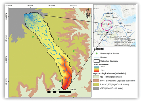
Suha sub-watershed is a portion of the fourteen Abay sub-basins called the North Gojjam sub-basins. The topography is undulating and variable, including rugged hills, mountains, and gentle plains. The watershed’s slope ranges from 0 to 50 percent, although the dominant slope class is 15 to 30 percent (Mekuriaw et al., 2020). In its relative location, the watershed is found in the southeastern part of Choke Mountain, which is the head of the Blue Nile/Abay in Ethiopia. Runoff from this watershed directly drains into the Abay River. The watershed has around 790 sq. km and is geographically located between 10°10’−10°40’ N latitude and 37°50’−38030’E longitude.

It is found in three traditional agro-climatic zones: Dega (2300–3200 m), Woina Dega (1500–2300 m), and Kolla (500–1,500 m) (G/Eyesus et al., 2003). A large segment of the watershed falls under the Woina Dega (69.04%) and Kolla (19%) agro-climatic zones. Dega (11.9%) takes up the remaining portion of the agro-climatic zone. Rainfall, in general, has an a bimodal nature in its temporal distribution: Kiremt and Belg, i.e., the area falls within Kiremt (the main rainfall season), Belg (the little rainfall season), and Bega (the dry season) in the area. The months with high temperatures in the study are from February to May, which is locally known as Belg (the little rainy season). In contrast, the coolest months are from October to January, which is termed Bega (the driest season). The area receives a mean annual rainfall of around 1021 mm. The average monthly maximum and minimum temperatures in the watershed vary from 9.4 °C to 25.1 °C, respectively.

The soil type and its characteristics are closely related to the parent material and the past geological processes that it has undergone at different times. According to FAO soil classification, the most dominant types in the watershed are nitosols and cambisols (Mekuriaw et al., 2020). These groups of soils constituted 47% and 31% of the study’s watershed, respectively.

In addition, vegetation cover and distribution patterns have a strong linkage with the climatic condition of an area in different parts of the earth. Thus, vegetation distribution in the area is highly governed by the type of local climatic conditions that exist at the specific site (agro-ecological zone). The lower altitude of the area, mostly classified as Kolla (low land), is covered with shrubs, bush, and stunted acacia vegetation, whereas the majority part, locally known as Woina Dega (midland) and Dega (highland), is dominated by vegetation like Bahir zaf (Eucalyptus), Tid (Juniperus procera), Zigba (Podocarpus gracilior), and kosso (Hagenia abyssinica) (Mekuriaw et al., 2020).

Administratively, the watershed is located in the east Gojjam zone of Amhara Regional State in North Western Ethiopia (Figure 1). It lies in four districts (woredas): Debay Tilatgin, Enemay, Shebel Berenta, and Dejen. According to the CSA (2007), the total population of the districts, including the capital, was 499,684. Females share slightly above half (50.8 percent) of their counterparts in the population. The estimated sex ratio was 97 males to 100 females. The most significant portion of the population (93.6 percent) lives in rural areas, whereas the remaining belongs to the urban group.

Figure 1. Location of Suha watershed.

Of the given total population, most of them engaged in agricultural (mixed) economic activities. Since the watershed has vast agricultural land, farmers cultivate various crop types, including cereals, legumes, oilseeds, and cash crops. The majority of the watershed’s area is used for agriculture, specifically crop cultivation and livestock rearing, which confirms the practice of mixed agricultural practice.

2. The land sat data and analysis method

2.1. LULC and NDVI data

This study employed a number of geospatial data for the land use land cover change and climate analysis, which were obtained from the United States Geology Survey (USGS) of the Earth’s Explorer website (https://earthexplorer.usgs.gov/) and other sources. The rationale for this is that it has the longest and most useful source of Earth’s data, with a medium to high spatial resolution of 30 m, and it is also freely available (Khun et al., 2021; Nayak, 2021). To identify the LULC, LST, and vegetation changes using normalized difference vegetation index (NDVI), the Landsat image of Operational Land Imager (OLI), Landsat 8, Enhanced Thematic Mapper Plus (ETM+), Landsat 7, and Landsat 5 Thematic Mapper (TM) were used (Table 3). The Landsat imageries were taken during the dry season for the 1990, 2000, 2013, and 2020 intervals, to get clear and visible images for the analysis. The selection of the years is based on major events such as forest resource management system change (1991), land redistribution in the Amhara region (1998), resettlement program in the Amhara region (2003), the introduction of the green economy (2010) and communal land distribution to the youth in the study area (2019). Dry season and cloud-free images were used to avoid the effect of seasonal variations (Kindu et al., 2013). In addition, the dry season is mostly considered as the best period to analyze differences among images. The time interval is set as nearly ten years, which is used in most LULC change analysis literature to detect and visualize the change (Belay & Mengistu, 2019; Eggen et al., 2016; Hassen & Assen, 2018). The area is covered with different types of land use types/classes (Belay & Mengistu, 2021; Yeneneh et al., 2022). However, some discrepancy in the time interval (+ or − 2/3 year) is taken into account due to the accessibility and quality of Landsat images from USGS archives for the study watershed.

Table 3. Description of the remotely sensed data

Satellite & sensor	Path	Row	Date of acquisition	Resolution	Source	Purpose
Landsat 5 TM	169	53	16/03/1990	30m	USGS	LULC & LST analysis
Landsat 7 ETM+	169	53	03/02/2000	30m	USGS	LULC & LST analysis
Landsat 8 (OLI)	169	53	08/01/2013	30m	USGS	LULC & LST analysis
Landsat 8 (OLI)	169	53	06/04/2020	30m	USGS	LULC & LST analysis
ENMA&KNMI			01/01/1990 30/12/2020	4km/month	ENMA/KNMI	Rainfall analysis

However, for the convenience of this study, the LULC pattern is characterized into six dominant classes: cultivated land, forestland, grazing land, built-up area, shrub/bushland, and bare land to see the direct correlation between climate elements (temperature and rainfall and NDVI) (Table 1).

Table 1. LULC changes categories in the study area

LULC classes	Description
Cultivated Land	Areas used for farmlands, small-scale irrigation, and the scattered rural settlements that are closely associated with the cultivated fields. These were combined into one class, as it was difficult to detect the dispersed rural settlements as a detached LULC class where fragmented cultivated land exists around settlements.
Forestland	Sites are relatively covered by dense forests with closed canopies (eucalyptus plantations found in homesteads and farmlands are also considered in this class).
Grazing land	Areas mainly covered with grasses and used as a source of animal feed and grazing field
Built up area	Areas with all types of artificial surfaces including residential areas (emerging rural towns, villages) occupied by living houses and constructions.
Shrub –bushland	Shrub-bushland dominated land with isolated small trees always with a lower range of grass.
Bare Land	Includes degraded areas, over-exploited cultivated farmlands, exposed bade rocks

Source: (Berhanu & Bisrat, 2018; Yeneneh et al., 2022 and local elders).

2.2. Image processing and classification

As a prerequisite, the pre-processing of the images includes layer-stacking, sub-setting, geometric correction, and radiometric correction tasks before the image classification and analysis work was done on each image to improve the quality of the image. To ensure uniformity amongst datasets during analysis, all satellite datasets were projected to the Universal Transverse Mercator map projection system zone 37N and World Geodetic System 84 (WGS84) datum (Belay & Mengistu, 2019). Layer stacking was carried out to convert multiple images into a single multi-band image layer. Since remotely sensed data are susceptible to distortions, haze, and noise reduction were applied to remove the possible distortions due to acquisition systems and platform movements (Girma et al., 2022). The study boundary is laid in different paths/rows; therefore, a raster mosaic was used to join the images and form a larger image. Image enhancement operations were performed using spatial enhancement tools such as the Convolution function to improve the quality of the raster image. Masking and removing of extraneous data were performed using the Subset and Chip tool (Ayele et al., 2019; Girma et al., 2022).

The land uses land cover image was classified using both unsupervised and supervised image classification approaches. Unsupervised classification is useful for quickly assigning uncomplicated and broad land cover classes such as water/land , vegetation/non-vegetation, forested/non-forested, etc (Madariya & Sharma, 2022; Regasa et al., 2021). This implies that LULC change analysis is an important technique to detect and describe the magnitude of vegetation cover change over the different spatiotemporal scales in response to human activities. The two biophysical components, vegetation, and climate have a direct relationship over an area (Schmidt et al., 2013). Change in vegetation coverage patterns brings some sort of variation in climate either at the local or regional level. Therefore, the images were passed through the required preprocessing and post-process operations.

Then, for a detailed investigation and understanding of a given land use type and its change through time, the pixel-based supervised image classification using a maximum likelihood classification algorithm was carried out. Supervised image classification is a recommended classification approach to have good results when adequate training data is available about the study area (Hussain et al., 2022; Yeneneh et al., 2022; Yesuph & Dagnew, 2019). The researcher intends to employ the Maximum Likelihood algorithm, assuming that it can effectively reduce classification error for classes. This method takes into account both the class covariance matrices and mean vectors as signatures, and involves merging constituent spectral class signatures to obtain rationalized class signatures (Belay & Mengistu, 2019, ; Yesuph & Dagnew, 2019).

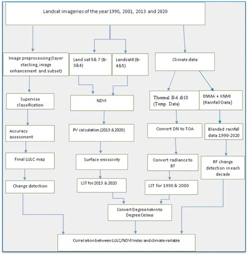
For each LULC type, training samples were selected by delimiting polygons around different demonstrative sites using Arc GIS 10.7.1 software (Nayak, 2021). Based on literature recommendations, 50 reference samples for each class were required and used for image classifications (Dibaba et al., 2020a). In addition, spectral signatures of different LULC classes resulting from the Landsat images were noted using the pixels enclosed by these polygons. Various band and color combinations were utilized to differentiate and interpret the surface aspects of the image during the process. The training data sets were often utilized for producing class signatures and classifying the entire image into useful information land use/type classes. Ancillary data such as topographic maps, GPS records, and the LULC history of the study area were gathered during field observation from elders and documents that were later used to complement the software-based classification task. A detailed flow of the work is depicted in the flow chart (Figure 2).

Figure 2. The overall work flow of the study.

2.3. Climate data (land surface temperature and rainfall)

2.3.1. Retrieving Land Surface Temperature (LST) from landsat image

Different researchers used various satellite images to drive land surface temperature (LST) like from land sat images and MODIS images (Guha et al., 2022; Hussain & Karuppannan, 2021; Mngube et al., 2020). However, the land sat image is the common one to estimate LST since it is easily accessible and a long period of image record is available from USGS respiratory. For this, the thermal infrared band 10 for Landsat 8 TIR image and band 6 for land sat 5/7 were used. For the bands that have a spatial resolution of 100 m, resampling was done using the nearest neighbor algorithm with a pixel size of 30 m to match the optical bands and make a suite for further analysis. To make further analysis of this variable, a stepwise operation was carried out as a prerequisite similar to the LULC image. Hence, the following steps were considered to correct the atmospheric distortion of the satellite data to estimate the LST from the TM, TM+, and OLI thermal bands (band 6 for land sat 5/7 whereas band 10 for land sat 8). First, estimating the spectral radiance of the image from the digital number of each pixel using Equation (1) was done. Satellite sensors measure the reflectance from the earth’s surface as digital numbers (DN) representing every pixel of the image (Guha et al., 2022; Yeneneh et al., 2022).

(1) $\lambda =\left(\frac{\mathrm{L}\mathrm{m}\mathrm{a}{\mathrm{x}}_{\lambda -}\mathrm{L}\mathrm{m}\mathrm{i}{\mathrm{n}}_{\lambda }}{\mathrm{Q}\mathrm{c}\mathrm{a}\mathrm{l}\mathrm{m}\mathrm{a}\mathrm{x}-\mathrm{Q}\mathrm{c}\mathrm{a}\mathrm{l}\mathrm{m}\mathrm{i}\mathrm{n}}\right)\ast \left(\mathrm{Q}\mathrm{c}\mathrm{a}\mathrm{l}-\mathrm{Q}\mathrm{c}\mathrm{a}\mathrm{l}\mathrm{m}\mathrm{i}\mathrm{n}\right)+\mathrm{L}\mathrm{m}\mathrm{i}{\mathrm{n}}_{\lambda }$(1)

Where Lλ represents spectral radiance, Cal= quantized calibrated pixel value in DN., Lmax =spectral radiance scaled to Qcal max in (watts/(m² × sr × μm)), Lminλ=Spectral radiance to Qcalmin in (watts/(m² × sr × μm)), Qcalmin=Minimum quantized calibrated pixel value (corresponding to Lminλ) in DN and, Qcalman=Maximum quantize calibrate pixel value (corresponding to Lminλ) in DN = 255.

But in the case of land sat 8 although bands 10 and 11 are allotted to thermal detection, band 10 is recommended to extract LST due to the high uncertainty in band 11 (Chibuike et al., 2018; USGS, 2019) and it is estimated by using the following formal (2)

(2) $L\lambda =ML\ast Q\mathrm{\_}cal+AL-O\mathrm{\_}i$(2)

Where Lλ =TOP spectral radiance (watts/(m² × sr × μm))

ML=Radiance multiplicative band (0.0003342), obtained from the Meta format of the image

AL=Radiance added Band (0.1), obtained from the Meta data of the image

Q_cal=quantize and calibrated standard product pixel values (DN)

Oi=correction value for band 10 which is 0.29, obtained from the Meta data of the image.

The second step is to convert the spectral radiance value to LST. Spectral radiance values for bands 10 and 11 were changed to radiant surface temperature under the assumption of uniform emissivity using pre-launch calibration constants for the Landsat 8 OLI sensor as indicated in Table 1. It is done by applying Plank’s inverse function (Chibuike et al., 2018) using the following Equal Meta data

(3) $\mathrm{B}\left(\mathrm{T}\right)Metadata\left(K\mathrm{\_}1/L\lambda +1\right)$(3)

Where BT=TOP of atmosphere brightness/effective at satellite temperature in kelvin

Lλ =TOP spectral radiance (watts/(m² × sr × μm))

K1 and K2 are constant values for (TM), (TM+), and (OLI), respectively as shown in (Table 2).

Table 2. The calibration constants for each sensor and selected thermal bands

Sensors with thermal bands	Constant1-K1(watts/(m^2 × sr × μm))	Constant 2- K2 (Kelvin watts/(m^2× sr × μm))	Rescaling factors for Landsat 8 (B10)
Landsat 5 (band 6)	607.76	1260.56	ML (Radiance mult. Band)	AL (Radiance add band)
Landsat 7 (band 6)	666.09	1282.71
Landsat8 (band 10)	774.89	1321.08	0.0003342	0.1

In the third step, the LST obtained from Landsat ETM + and OLI/TIRS was converted into degrees Celsius (C°) for easy understanding (4) (John et al., 2020; Merga et al., 2022).

(4) $LST\left({ }^{\mathrm{o}}C\right)=T\left(K\right)-273.15$(4)

However, to get the LST from Land sat eight and from band ten, it requires to proceed an additional step keeping the previous steps as it is. Hence, the fourth step is estimating the land surface emissivity (E) of an image, which plays a significant role in the existing surface temperature of that site. It is calculated by using the normalized difference vegetation index (NDVI) and the appropriate bands for NDVI estimation (Chibuike et al., 2018; Merga et al., 2022). Hence, the PV value is calculated by using the following equation (5).

(5) $E=0.004\ast PV+0.986$(5)

Where E=land surface emissivity, 0.004 and 0.986=correspond to a correction value, PV=proportion of vegetation which is obtained (Gohain et al., 2021; Merga et al., 2022) using the following equation (6)

(6) $\text{PV}=\left[-0.15em\left[\text{NDVI-NVI}\right]-0.15em\right]\_\text{min}/\left[-0.15em\left[NDVI\right]-0.15em\right]\_\text{max}-\left[-0.15em\left[\text{NDVI}\right]-0.15em\right]\_\text{min}$(6)

Where PV= proportion of vegetation, NDVI=DN values for NDVI image, NDVI_min =Minimum DN values from DNVI image, and NDVI_max=Maximum DN values from DNVI image

For this, the NDVI value should be calculated using the red band (B-4) and the near-infrared band (B-5) of land sat 8 respectively using the following equation (7) (Merga et al., 2022; Tan et al., 2020).

(7) $NDVI=\left(\left(Band5-Band4\right)/\left(Band5+Band4\right)\right)$(7)

The last step is calculating the land surface temperature (LST) from band 10 based on the above results (Eq.2, Eq.3, and Eq.5) by applying the following Eq.8.

(8) $LST=BT/\left(\left(1+\left(\lambda \ast BT/c2\right)\ast \mathrm{l}\mathrm{n}\left(E\right)\right)\right)$(8)

Where LST= land surface temperature

BT= top of atmosphere brightness temperature (${ }^{\circ }\mathrm{C}$), λ=wavelength of emitted radiance, C₂=h*c/s which is 1.4388 × 10² mk = 14388mk, h=Planck’s constant = 6.626 × 10⁻³⁴ JS, S=Boltzmann constant = 1.38 × 10⁻²³Jk and C= velocity of light = 2.998 × 10⁸ m/s.

2.3.2. Retrieving the rainfall data

The rainfall data (1990–2020) were obtained from the Ethiopian National Metrological Agency (ENMA) and KNMI. The study obtained and used 4 km × 4 km reconstructed (blended) mean monthly rainfall data of the weather station records with the satellite estimate from ENMA of the year 1990 to 2015 and from KNMI of the year 2016 to 2020. The gridded data set is very useful in areas where the weather stations are limited in number and distribution, a missing data problem, and a short period of observation. Gridded rainfall records archived in the KNMI port were mainly taken from Cen Trend v1 and Climatic Research Unit Time-Series (CRU_TS) 4.04. This is also the most complete and updated dataset of gridded precipitation at the global scale, has a spatial resolution of up to 0.25, and covers the period from 1901 to now (Tsidu, 2012).In areas where there are insufficient weather stations and uneven distribution, as well as short observation records, the gridded data comes in helpful.

2.3.3. Estimation of NDVI

NDVI is one of the most widely used remote-sensing vegetation indices to identify the coverage of vegetation based on spectral values (Mngube et al., 2020). It is a biophysical parameter, which relates to photosynthetic vegetation to offer valuable information about the dynamics of vegetation covers over time. The main principle in using NDVI value is that vegetation leaves are highly reflective in the near-infrared and highly absorptive of the vegetation pigments (chlorophyll) in the visible red (Debie et al., 2022). The contrast between these channels can be used as an indicator of the status of the vegetation. The NDVI values were estimated as follows (Mohammed et al., 2019):

(9) $NDVI=\left(NIR-RED\right)/\left(NIR+RED\right)$(9)

where NIR is a near-infrared band (TM and ETM band 4, OLI band 5) as well as R is the red band (TM and ETM band 3, OLI band 4). The NDVI was estimated using ArcMap from Landsat images and expressed in a value between − 1 and 1.

2.3.4. Accuracy assessment

In the post-classification process, evaluating the accuracy of classification is fundamental work to validate the correctness of the work. For this validation, a set of reference points (240) were taken from the classified image which is independent of the training GPS points, as well as spatially and temporally distributed in the whole watershed and categorically encompassing all LULC types (Yesuph & Dagnew, 2019). The reference points were collected from the corresponding Google Earth, original Landsat images, previous reports and maps, and field observations. For instance, a topographic map of the years 1990, 2000, and 2013 was obtained from the Ethiopian Mapping Agency as a reference point to validate the classification process. Information from old age and informed people as well as corresponding high-resolution Google Earth images were also used for the years 1990, 2000, and 2013 as an additional source of data to validate the classification process. Also, field visits were used to collect sample points for the 2020 reference year (Belay & Mengistu, 2019). After this, the error matrix was calculated to see the overall accuracy and kappa coefficient by using the following Equation (10) and (11).

(10) $\mathrm{O}\mathrm{v}\mathrm{e}\mathrm{r}\mathrm{a}\mathrm{l}\mathrm{l}\mathrm{u}\mathrm{r}\mathrm{a}\mathrm{c}\mathrm{y}=\frac{\mathrm{n}\mathrm{u}\mathrm{m}\mathrm{b}\mathrm{e}\mathrm{r}\mathrm{o}\mathrm{f}\mathrm{s}\mathrm{a}\mathrm{m}\mathrm{p}\mathrm{l}\mathrm{i}\mathrm{n}\mathrm{g}\mathrm{c}\mathrm{l}\mathrm{a}\mathrm{s}\mathrm{s}\mathrm{e}\mathrm{s}\mathrm{c}\mathrm{l}\mathrm{a}\mathrm{s}\mathrm{s}\mathrm{i}\mathrm{f}\mathrm{i}\mathrm{e}\mathrm{d}\mathrm{c}\mathrm{o}\mathrm{r}\mathrm{r}\mathrm{e}\mathrm{c}\mathrm{t}\mathrm{l}\mathrm{y}}{\mathrm{n}\mathrm{u}\mathrm{m}\mathrm{b}\mathrm{e}\mathrm{r}\mathrm{o}\mathrm{f}\mathrm{r}\mathrm{e}\mathrm{f}\mathrm{e}\mathrm{r}\mathrm{e}\mathrm{n}\mathrm{c}\mathrm{e}\mathrm{s}\mathrm{a}\mathrm{m}\mathrm{p}\mathrm{l}\mathrm{i}\mathrm{n}\mathrm{g}\mathrm{c}\mathrm{l}\mathrm{a}\mathrm{s}\mathrm{s}\mathrm{e}\mathrm{s}}$(10)

Then, the overall accuracy, Kappa coefficient, producer’s accuracy, and user’s accuracy were calculated from the error matrix (Kebede, 2018; WoldeYohannes et al., 2018; Yesuph & Dagnew, 2019). The overall accuracy of the classification was computed by dividing the number of correct values in the diagonal’s matrix by the total number of values, which were taken as a reference point. On the other hand, the producer’s accuracy is derived by dividing the number of correct pixels in one class by the total number of pixels as derived from reference data. Also, the user’s accuracy was calculated by dividing the correct classified pixels by the total number of pixels, and the Kappa coefficient, which measures the agreement between the classification map and the reference data was calculated (WoldeYohannes et al., 2018).

(11) $kappacoefficient\left(K\right)=\frac{observedaccuracy-chanceassessment}{1-chanceagreement}$(11)

Kappa coefficients typically lie between zero and one. According to Dibaba et al. (2020a), a kappa value that is characterized as greater than 0.8 denotes a strong agreement, a value between 0.4 and 0.8 denotes a moderate agreement, and a value below 0.4 represents a poor agreement.

2.3.5. Spatio-temporal distributions of LULC change detection

One of the post-classification tasks is to conduct change detection among the different images which was carried out by comparing the LULC image on a pixel-by-pixel basis at different time scales (WoldeYohannes et al., 2018). After the classification has been done the change/difference is detected from 1990 to 2020 by breaking it into almost three decades (1990–2000, 2001–2013, and 2014–2020) using the change rate in percent for each type of land use and land cover. Hence, to determine the magnitude, trend, and rate of land use/land cover changes in the watershed, the area comparison analysis was made by subtracting the total area of each class (Yesuph & Dagnew, 2019). The rates of change of LULC classes and their percentage were therefore determined by the following Eq.:

(12) $C=\left(A_{t2}-A_{t1}f\right)/A_t\ast 100$(12)

where A_t1 is the area of land use under one class in time t1; A_t2 is the area of the same type of LULC in time t₂, A_t is the total area of the catchment and C is the rate of change in percent (Hassen & Assen, 2018).

2.3.6. Correlation between LULC (NDVI) and climate variables

After the LULC change classification, NDVI and climate trend analysis were done. This was again followed by a correlation analysis. It was carried out between LULC change and climate variables (LST/rainfall) by using Pearson correlation Spearman (PCC). The NDVI values, which were derived from each LULC class, were employed on the side of LULC change. A linear regression analysis model was also employed to identify the coefficient of determination between the LULC and climate variables in the study within the given period. The PCC model is given as follows;

(13) $r_{xy}=\frac{{\sum }_{i=1}^n\left(xi-xm\right)\ast \left(yi-ym\right)}{\sqrt{{\sum }_{i=1}^n{\left(xi-xm\right)}^2+{\sum }_{i=1}^n{\left(yi-ym\right)}^2}}$(13)

where r_xy is the simple correlation coefficient of variables x and y, xi is the NDVI or vegetation cover of the i^th year/month, yi is the climatic element (LST/RF) of the i^th year/month, xm is the average NDVI or vegetation cover for all years/months, ym is the average LST/RF for all years/months (Li et al., 2004).

It was applied to each pixel using Statistical Software of Microsoft Excel (XLSTAT version 19 software (Nega et al., 2019). It is a statistical measure of the strength of a linear relationship between paired data. The coefficient values range from −1 to 1, where 1 indicates a perfect positive relationship, −1 indicates a perfect negative relationship and 0 indicates no relationship exists (John et al., 2020; Nayak, 2021). The Evans standard leveling method (Evans, 1996) was used to calculate Pearson’s correlation value in the matrix and the strengths of the coefficient of determination (R²) for the regression model. The t-test distribution was used to determine the statistical significance of the trend and correlation coefficient values (Table 4).

Table 4. The correlation coefficient (r) and the coefficient of determination (R²) categorical values

Level of statistical strength	r value (absolute)	R^2
Very weak	0.00–0.19	0.00–0.036
Weak	0.20–0.39	0.04–0.15
Moderate	0.40–0.59	0.16–0.35
Strong	0.60–0.79	0.36–0.63
Very strong	0.80–1.00	0.64–1.00

Generally, to see the overall flow of the analysis work, based on the sub-specified objectives, the following sketch was developed. LULC, NDVI derived from each LULC, LST, and rainfall were the main components/variables in this study (Figure 2).

2.3.7. Prediction of LULC dynamics

Prediction of LULC change is one of the most important tasks among environmentalists to make appropriate plans and decisions in related resource management and conservation (Baig et al., 2022).LULC dynamic is governed by many biophysical and socio-economic variables. Hence, identifying the most influential factors based on the study area context before the prediction is a viable task.

2.3.8. Driving factors and model specification

Predicting LULC change (dependent variable) is determined by several biophysical and socio-economic variables (Girma et al., 2022). These factors had a substantial impact on land use and land cover patterns in the past. As a result, the driving variables (independent variables) were used for simulating the LULC dynamics (Hussien et al., 2023). The physical variables included in the model calibration were chosen because of their significant relation with LULC dynamics, which includes elevation, slope, and distance from the stream/rivers. The elevation is recognized as the imperative topographic factor affecting LULC change. Slope affects the spatial trends of land cover change suppose that the gentler a land slope is, the easier it is to have land use changes. Also, river proximity provides convenience to residents to access resources while changing land (Girma et al., 2022; Hussien et al., 2023).

On the other hand, socioeconomic factors such as population density, distance from the urban/city center, and distance from the road were also considered since they play a significant role as a driving force in affecting the landscape pattern of land use land cover. Population density is the most prominent anthropogenic factor in land use change where the higher the density more frequent land use change. Anthropogenic disturbance has a strong association with the land cover type. Distance from urban can be taken as a very strong driver for land use land cover change where the closer the land to the urban center is the easier for land use change. Distance from the road also determines accessibility to different sites, which is one of the major drivers in attracting more urban users and expansion.

A digital elevation model (DEM) of 30 m resolution from the Advanced Space borne Thermal Emission and Reflection Radiometer (ASTER) was used to prepare the elevation, slope, and stream network of the study watershed (https://earthexplorer.usgs.gov/). However, road network, population density, and urban/city centers were obtained from this site (https://www.diva-gis.org/gdata). Consequently, these data sets were produced using ArcGIS software and then exported to QGIS version 2.8.3 to run the potential transition maps using the MOLUSCE plugin. All variables were standardized into the same number of scales (classes) and geographical projections in the way that fit the models.

Although numerous prediction models exist, the artificial neural network (ANN) model was utilized in combination with cellular automata (CA) to anticipate land use changes. An artificial neural network (ANN) is a computational model that can perform tasks such as prediction, classification, and decision-making (Baig et al., 2022; Bhartendu et al., 2022; Leta et al., 2021). It has a dynamic simulation capacity, high efficiency of performance with limited data, simple calibration steps, and the ability to reproduce different LULC and complicated patterns. The model combines the CA and Markov chains to model land use changes across network categories (Baig et al., 2022; Bhartendu et al., 2022). The CA-ANN model is coupled with the MOLUSCE Module (QGIS Plugin), which was recently made available to evaluate present LULC changes and estimate future LULC. It has four different models: Multi-Criteria Evaluation (MCE), Artificial Neural Networks (ANN), Logistic Regression (LR), and weights of evidence (WoE). This module may use the Markovian technique to generate a transition potential/possibility matrix and train a simulation model (Bhartendu et al., 2022).

3. Result and discussion

3.1. Land Use-Land Cover (LULC) changes

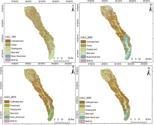
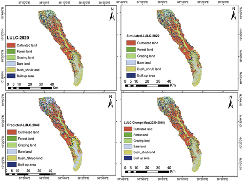
A pixel-based supervised image classification with a maximum likelihood algorithm was used to classify the land sat images and by considering the interest of the study, six dominant LULC classes were generated. Few other LULC classes can be generated but their proportion is insignificant to give classes. For that, those undefined pixels have been incorporated within neighboring classes within the system. The ultimate classification products provided an impression of the major LULC features of the study area from 1990 to 2020. Cultivated land, the dominant land use type of the catchment, covered 43.99% in 1990, 51.16% in 2000, 57.90% in 2013, and 60.83% in 2020 respectively (Table 5). The proportion of bare land in 1990, 2000, 2013, and 2020 was 7.43%, 8.03%, 8.06 and 8.96 % of the total area, respectively. The built-up area covered 7.14%, 8.54%, 8.91%, and 9.07% area of the catchment in 1990, 2000, 2013, and 2020, respectively. This figure indicated that both bare land and built-up areas increased from 1990 to 2020. However, forestland, grazing land, and shrub-bush land area showed a decreasing trend in the above respective years. For instance, from 1990 to 2020, forestland decreased from 6.89% to 3.93% in the study area. Similarly, grazing land in the years 1990, 2000, 2013, and 2020 was 18.94%, 12.56%, 9.72%, and 7.08% respectively. In addition, bush-shrub land in 1990, 2000, 2013, and 2020 was 15.62%, 14.21%, 11.16%, and 10.13% respectively. For the period 1990 to 2020, grazing land, bush-shrub land, and forestland experienced the greatest drop, while cultivated land experienced the greatest gain. In the research area, the LULC was higher for changes from 2013 to 2020 than for changes from 1990 to 2000 and 2001 to 2013.

Table 5. LULC areal distribution from 1990 to 2020 in the study watershed

LULC type	Area
	1990		2000		2013		2020
	Ha	%	Ha	%	Ha	%	Ha	%
Cultivated Land	34729	43.99	40391	51.16	45715	57.90	48025	60.83
Forest	5436	6.89	4340	5.50	3357	4.25	3106	3.93
Grazing land	14953	18.94	9920	12.56	7673	9.72	5587	7.08
Bare land	5864	7.43	6342	8.03	6362	8.06	7075	8.96
Bush-shrub	12332	15.62	11218	14.21	8811	11.16	8001	10.13
Built-Up	5637	7.14	6740	8.54	7033	8.91	7157	9.07
Total	78951	100	78951	100	78951	100	78951	100

The distribution of LULC change over the last thirty years is also depicted on the map (Figure 3). As the figure depicted, expansion in agricultural land, bare land, and built-up showed a continuous increment whereas forestland, grazing land, and bush-shrub land depicted a continuous decline in the study area over the given period. To understand this, the spatiotemporal distribution of the LULC in the Suha watershed is presented in Figure 3. Mostly, the expansion of the cultivated land was at the expense of the forestland, grazing land, and bush-shrub land in the catchment. Due to this most of these land, use classes were converted to cultivated, bare, and built-up areas in the study area. The finding of this study agrees with those previous LULC change research reports conducted within the various watersheds of the Blue Nile basin and other parts of the country. Most of the findings of this research documented the continuous expansion of farmlands/built-up areas at the expense of other land use/cover types particularly forest and grazing land workflow (Dibaba et al., 2020a, ; Mekuriaw et al., 2020; WoldeYohannes et al., 2018). According to Dibaba et al. (2020a), the reason behind this is that there is a continuous demand for agricultural and settlement/built-up areas in most of the country including the study area due to high population growth.

Figure 3. LULC maps for the years 1990, 2000, 2013, and 2020 of Suha watershed.

The spatial rate of change analysis over the study period showed that the cultivated and grassland showed a high rate of conversion during the first decade of the study period in which the cultivated land gained about 38.04% of land from the others, whereas the grassland losses about 33.81% to the others LULC from 1990 to 2000. In this period, the least change was observed in the bare land (4.55% gained) in the area (Table 6). Similarly, cultivated land, bushland, and grassland experienced very dramatic changes between 2001 and 2013 in the area. Cultivated land showed the highest rate of change and gained about 48.08% of the land, whereas bush-shrub land declined by 21.74% followed by grazing land by about 20.29% in this time scale, the least conversion was observed on bare land (0.18% gain) as the previous time. Between 2013 and 2020, grassland lost the highest percentage of the land (33.14%) whereas cultivated land gained the percentage of the land (36.7%) as compared to the other land use classes. The minimum change was identified in the built-up area during this period, which was a 1.97% gain. When the overall change is assessed from 1990 to 2020, more or less cultivated and grazing land showed a high change as compared to the others. Cultivated land gained about 41.48% of land from others, whereas grazing land shrank by 29.22% of land in the study area. Bare land showed less change even in the whole period of analysis (3.78% gained). The FGD participants and elders revealed that LULC changes are driven by both anthropogenic and natural causes. As a comparison to the natural causes, anthropogenic activities were found the main drivers of LULC change. High demand for agriculture, population growth, wood extraction, urban expansion, and a lack of continued environmental conservation were some of the identified drivers in the area.

Table 6. LULC change analysis from 1990 to 2020 in the study watershed

LULC type	Change detection (loss/gain)
	1990–2000		2001–2013		2013–2020		1990–2020
	Ha	%	Ha	%	Ha	%	Ha	%
Cultivated Land	5662	38.04	5324	48.08	2310	36.70	13296	41.48
Forest	−1096	8.71	−983	7.07	−251	3.99	−2330	7.27
Grazing land	−5033	33.81	−2247	20.29	−2086	33.14	−9366	29.22
Bare land	478	4.55	20	0.18	713	11.33	1211	3.78
Bush-shrub	−1114	7.48	−2407	21.74	−810	12.87	−4331	13.51
Built-Up	1103	7.41	293	2.65	124	1.97	1520	4.74

The changing trend indicated that cultivated land, bare land, and built-up areas showed an increasing trend whereas the other land use types manifested more or less a decreasing trend across the reference period (Figure 4 and Table 6). The findings are consistent with study reports indicating that agricultural expansions and increased human settlement, driven by rapid population growth, significantly accelerate the LULC shift in many parts of Ethiopia and other regions of the country (Merga et al., 2022; Nayak, 2021, Tewabe & Fentahun, 2020; WoldeYohannes et al., 2018). The reason behind this was partly related to the change of land use policy, which led to the redistribution of grazing land and clearance of shrubs for the expansion of farmlands and new settlement centers at different times. These revealed that further vegetation clearance in search of additional farmlands, new settlement units, and grazing could eventually transform the initial extents of all land use land covers into another type in addition to the natural factors (Hassen & Assen, 2018; Yeneneh et al., 2022; Yesuph & Dagnew, 2019).

Figure 4. LULC change from 1990 to 2020 in Suha watershed.

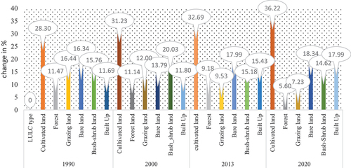
The extent of LULC change (from 1990 to 2020) can also be easily visualized using the following bar graph (Figure 4). As the graph shows cultivated land showed a continued increase followed by bare land whereas the grazing and forest land showed continued decreasing pattern over the study period in the watershed.

3.2. The accuracy assessment result

In order to verify the accuracy of classification, more than 240 validation points, which were geographically and temporally spread in the whole watershed and categorically comprising all LULC types were created by stratified random sample technique (Yesuph & Dagnew, 2019). Corresponding high-resolution Google Earth images were used as additional sources of information that supported the validation process. Then the accuracy assessment result was identified as the user, producer, and overall accuracies, in addition to the kappa coefficient (Table 7). The overall accuracy and kappa statistics were applied to assess classification accuracy. The producer and user accuracies of both classes were consistently high (Rwanga & Ndambuki, 2017; Tewabe & Fentahun, 2020). The overall accuracy for the 1990, 2000, 2013, and 2020 maps was 89%, 90%, 92%, and 91%, respectively. The Kappa statistics were 0.81, 0.86, 0.84, and 0. 82 for the 1990, 2000, 2013, and 2020 maps, respectively. The Kappa statistics showed a strong agreement for the years 2000, 2013, and 2020, respectively.

Table 7. Summary of the accuracy assessment result in the study watershed

LULC type	1990		2000		2013		2020
	UA	PA	UA	AP	UA	AP	UA	AP
Cultivated Land	90.79	91.21	91.31	93.45	93.74	93.19	94.23	92.41
Forest	92.71	89.16	89.26	84.46	92.91	86.93	70.56	85.82
Grazing land	80.82	80.38	80.48	90.72	94.35	77.65	90.21	75.43
Bare land	77.76	80.32	80.42	77.79	69.36	78.65	72.14	86.04
Bush-shrub land	94.65	93.68	93.78	95.01	94.43	94.43	93.19	90.76
Built-Up	73.86	95.54	95.89	76.27	89.47	95.01	95.32	91.23
Overall accuracy (%)	0.89		0.90		0.92		0.91
Kappa coefficient.	0.81		0.86		0.84		0.82

3.3. The trend of the Normalized Vegetation Index

In remote sensing, each land use/cover has a distinct interaction with the electromagnetic spectrum; thus, such surface features could be captured in the satellite image and recognized using spectral indices such as the NDVI transform (Hereher, 2017; Nega et al., 2019). This is because it enables us to detect the land use and land cover change in a given area within a specified time. NDVI value estimation is assessed based on the spectral properties of vegetation i.e. it depends on its absorption of visible light, energy used in photosynthesis, and reflected near-infrared (NIR) radiation. In this study, the NDVI value of the study area was derived using Landsat images of the years 1990, 2000, 2013, and 2020 as shown in Figure 5. To do this, ERDAS Imagine 2015 software was mainly used and the NDVI value was found between −0.14 to + 0.74 in 1990, and from −0.09 to 0.68 in 2000, respectively, in the study area. Figure 5 also depicted that in 2013, NDVI values changed (minimum −0.04 to maximum + 0.46), and in 2020, the NDVI value was found from −0.08 to 0.55 in the area. Higher NDVI values showed that there is more health and better coverage of vegetation, and forest/grasses in the area whereas lower values of NDVI showed that there is unhealthy and less vegetation coverage in the area. Environmental change/conversion from one land use/land cover to the others (from forest/grazing land to cultivated Land, build-up area, or bare land) is one of the prominent factors. Therefore, the NDVI map of Figure 5 showed a major decrease from the initial to the last period set for this study in the watershed. Overall, the maximum NDVI value was observed in 1990, when more forest, grazing, and bush-shrub land was available than in the other periods. When bare soil, built-up area, and cultivated land are enlarged, the vegetation cover becomes shirked, which in turn influences the value of NDVI in recent times as compared to the previous one in the area. The trend of NDVI value for each LULC in each decade also confirmed that it declined from time to time (Table 8).

Figure 5. The NDVI maps of the years 1990, 2000, 2013, and 2020 in Suha watershed.

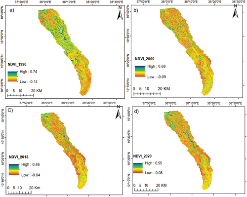
Table 8. The relative change and correlation between NDVI and climate variables from 1990–2020

Year	Cultivated (NDVI)	Forest (NDVI)	Grazing land (NDVI)	Bare land (NDVI)	Bush shrub land (NDVI)	Built up (NDVI)	LST	RF
1990	0.22	0.45	0.38	0.20	0.30	0.25	25.66	1060.84
2000	0.25	0.23	0.28	0.15	0.31	0.23	27.02	1056.52
Change	0.05	−0.22	−0.10	−0.05	0.01	−0.02	1.36	−4.31
2013	0.10	0.22	0.21	0.14	0.13	0.17	30.04	1053.93
Change	−0.10	−0.23	−0.07	−0.02	−0.18	−0.08	3.02	−2.60
2020	0.09	0.12	0.15	0.17	0.11	0.13	32.17	1049.99
Change	−0.02	−0.10	−0.06	0.03	−0.03	0.04	2.13	−3.94

3.4. Land Surface Temperature (LST) changes

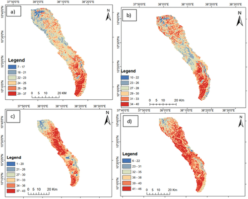
The mean LST of the study watershed in the last 30 years showed a steady increase, which is consistent with the global warming trend (Tan et al., 2020). This was mainly observed when we calculated the LST for each land use/land cover class (Table 44). Fig. 45 also depicted the spatial and temporal pattern of LST in the years 1990, 2000, 2013, and 2020 in the Suha watershed. The value of LST was found to be 7–37°C in 1990, 10–40°C in 2000, 1–43°C in 2013, and 6–46°C in 2020, respectively. The increasing trend of LST would be associated with the drastically changing and degraded area of the site, which could be manifested by the expansion of bare land and build-up from 1990 to 2020. Comparatively, the upper part of the study area exhibits a lower temperature due to relatively higher vegetation coverage and high-altitude effect. In contrast, the central part exhibits somewhat rising LST due to rapid urban expansion and shrinking vegetation cover, particularly from 2013 onwards. The highest deviation was noticed in maximum and minimum temperatures for the year 2020 (46°C) and (6°C), respectively (Figure 6). Although there exist some limitations on the remotely sensed LST-derived data, the recorded LST is acceptable and can be used for further analysis in temperature variability/change in the study area. Furthermore, the maximum LST values in the area were observed among the central part in which high urbanization and quick infrastructure expansion were observed, representing a positive relationship between LST and built-up area. A study conducted both globally and locally came to a similar conclusion, stating that increasingly built-up areas and barren lands have the greatest LST, whereas the temperature in vegetated rural areas tends to drop (Karakuş, 2019; Nega et al., 2019; Regasa et al., 2021; WoldeYohannes et al., 2018).

Figure 6. The LST maps of the years 1990(a), 2000(b), 2013(c) and 2020(d) in Suha watershed.

3.5. Rainfall changes and trends

The Mann-Kendall trend test (MK) and Sen Slope estimator were used to see the time-series data from 1990 to 2020 in the study watershed to see the seasonal and annual rainfall trends. The trend analysis was done for the mean annual and summer (main rainy season) rainfall in each decade in the given period. The MK results test revealed that during the annual and Kiremt season (0.78 mm/season), a statistically non-significant decreasing trend (1.056 mm/year) was observed at 0.05, respectively. Not only the temporal trend but also the spatial distribution of it showed a significant variation from time to time in the upper, middle, and lower parts of the watershed (Figure 7).

Figure 7. The rainfall maps of the year 1990, 2000 2013, and 2020 in Suha watershed.

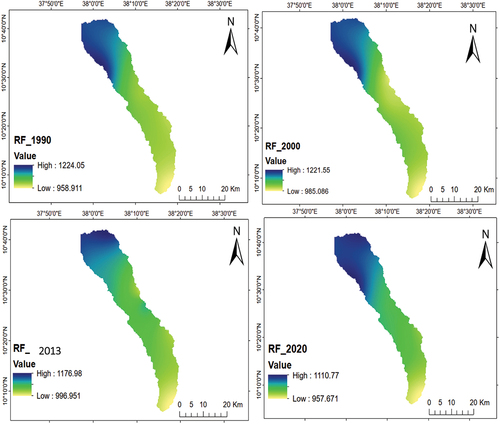
This implies that the decreasing trend of rainfall during the main rainfall (kiremt season) season brought a significant impact on the mean annual rainfall trend and pattern over the given period. Other seasons such as spring (Belg-little rain season) and winter might show an increasing trend but the impact would be much less as compared to the main rainfall season. The results are consistent with the findings of Asfaw et al. (2018) who found a statistically significant decreasing trend of the summer and annual rainfall with a rate of 15.03 and 13.12 mm per decade, respectively, in the north-central part of Ethiopia. Furthermore, a study conducted by Feke et al. (2021) at Horro Guduru in the northwestern parts of Ethiopia revealed that declining annual rainfall was observed over the last 33 years.

3.6. Relationship between LULC vs. Climate variables

The changes in LULC have a considerable influence on local climate variability, especially in agricultural and urban areas. It is one of the main driving forces for global climate change. For example, the change from vegetation to urban built-up causes not only interruptions of carbon and water cycles but also affects the energy fluxes between the land and the atmosphere (Hereher, 2017). For this, NDVI has been widely used as an indicator of vegetation abundance to estimate LST in different studies (Regasa et al., 2021; Xiao & Weng, 2007). The correlation analysis was done, and its mean coefficient reached as high as 0.40 (Table 4). Hence, the correlation between LULC change and major climate elements such as LST and rainfall can be examined by an analysis of the changes in NDVI.

3.7. LST vs NDVI (LULC)

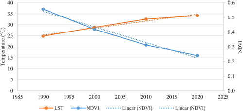
The result presented in Table 8 and Figure 10 showed the relative change and correlation between the mean value of LST, and different categories of land use land cover NDVI (taken in the dry season) classes in each decade in the study watershed. Based on the results obtained from each land use/cover class, cultivated land (0.22 & 0.25), bare lands (0.2 & 0.15), and built-up area (0.22 & 0.25)) showed the lowest NDVI value in 1990 and 2000 years respectively (Figure 5). Also, in the last two decades (2013 and 2020), a similar situation was observed among the above land use categories with some differences in their NDVI value. On the other hand, forest land, grazing land, and grassland had a higher value in the same two decades, where there was some disparity in the recent two decades (2013 and 2020). The trends in NDVI value also indicated the highest and lowest change between 1990 and 2020, in which the highest was in forestland (0.33), whereas the lowest was observed in bare land (0.03) among the different LULCs. In general, the overall pattern of NDVI values decreases from 1990 to 2020 almost in all LULCs in the study area. Furthermore, the mean total annual LST of the area showed an increasing trend from 1990 to 2020 in the watershed. When the mean annual temperature was low, the NDVI of all land cover categories was high (Table 8). On the contrary, when the mean annual temperature was high, the NDVI of all land cover categories was low. For instance, the mean annual temperature increases of 1.36 ̊C, 3.02 ̊C, and 2.13 ̊C were observed from 2000 to 1990, from 2013 to 2000, and from 2020 to 2013, respectively, in the study sub-watershed. This means that an inverse relationship was observed between the two groups of variables (LST and NDVI). A similar finding was also found and stated that the NDVI value of a LULC was high while LST was low in areas where there is better coverage of vegetation/grasses while the LST and on times when greenness increases. With an increase in the NDVI, the mean LST decreased significantly, which means they are negatively correlated with the mean LST (Tan et al., 2020; Yue et al., 2007).

The analysis further suggested that the mean variation of LST due to the change in NDVI value of the different LULCs, particularly in the dry season was explained based on the coefficient of determination that ranges from moderate to the highest values (Table 9). The highest variation was observed on grazing land (R² = 0.92), forestland (R² = 0.86), and cultivated land (R² = 0.94), in the study area. The correlation between LST and those LULCs was statistically significant (p = 0.05). On the other hand, moderate variation in LST related to NDVI was seen among bare land (R² = 0.31), bush-shrub land (R² = 0.64), and builtup area (R² = 0.82) in the study period. Temperature variation throughout the given period showed relatively moderate in the 1990s and 2000s whereas it showed a greater variation from 2010 to 2000 among the different LULCs in respective to their NDVI values.

Values in bold are different from 0 with a significance level of alpha = 0.05

Regarding the Pearson’s correlation coefficient between mean temperature and land use/land cover (cultivated Land, forestland, grazing land, bare Land, bush shrub, and built-up area), the NDVI value was negative 0.97, 0.93, 0.96, 0.55, 0.80 and 0.91, respectively. In the study area, the increasing temperature affected the NDVI value negatively.

3.8. Rainfall vs. NDVI (LULC)

The analysis between rainfall and NDVI showed from modern to strong correlation among the different land use/land cover classes in the study area. Table 8 and Table 9, of the Pearson correlation coefficient between mean annual rainfall and each LULC (cultivated Land, forest land, grazing land, bare Land, bush shrub, and built-up area) of NDVI was found to be 0.91, 0.96, 0.95, 0.64, 0.67 and 0.95, respectively. The results are statistically significant with forestland, grazing land, and built-up area, and it is positively correlated with the all-land use/land cover category. Like in the case of LST, dry season NDVI data was used to show the impact and association of vegetation cover on rainfall because only vegetation that is entirely independent of precipitation survives in the dry season, but others, like grasses and crops, dry out. Furthermore, the mean total annual rainfall of the area showed a decreasing trend from 1990 to 2020 in the area as indicated in Table 8. When the mean annual rainfall was high, the NDVI of all land cover categories was high, and vice versa is true (Table 8). For this, a decrease of 4.31 mm, 2.6 mm, and 3.94 mm in rainfall was observed from 2000 to 1990, from 2013 to 2000, and from 2020 to 2013, respectively, in the study sub-watershed. The result further showed that the rainfall of each LULC’s NDVI was positive. Previous studies also indicated that dry season NDVI value showed the impact of changes in vegetation cover on the rainfall trend of an area because only vegetation that is entirely independent of rainfall exists in the dry season but others like grasses/crops couldn’t (Gohain et al., 2021; Hussain & Karuppannan, 2021; Nega et al., 2019).

Table 9. Correlation matrix & coefficient of determination (Pearson) b/n mean climate variables & NDVI value of each LULC (1990 to 2020)

Description of r/n	Variables	Cultivated (NDVI)	Forest (NDVI)	Grazing (NDVI)	Bare (NDVI)	Bush Shrub (NDVI)	Built up (NDVI)
Correlation matrix	LST	−0.97	−0.93	−0.96	−0.55	−0.80	−0.91
	RF	0.91	0.96	0.95	0.64	0.67	0.95
Coefficient(R^2)	LST	0.94	0.86	0.92	0.31	0.64	0.82
	RF	0.83	0.92	0.90	0.41	0.44	0.90

3.9. Prediction of land use land cover change

The CA-ANN model was used to describe the changing potential of the predicted LULC dynamics from the artificial neural network (ANN) learning process. Primarily the model requires historical LULC data sets which have an initial (2014) and final (2020) year and variables that include both the physical (slope, distancefrom river,) and socio-economic (distance from road , distance from existing population density) as depicted in Figure 8. This model utilized those data as inputs to produce a simulation land use land cover dynamic map and changing matrix between 2014 and 2020 before the actual prediction was done between the years 2020 and 2040. The MOLUSCE plugin in QGIS was used to carry out this operation. The plugin also produces a transition probability matrix that shows the proportion of classes that have changed from one category to the other and calculates the proportion of area changes in a particular year. Additionally, the plugin created a change map from 2014 to 2020 for each land use land cover class. In the cellular automaton-Artificial neural network (CA-ANN) model, the ANN-Multi-layer perception method was used to predict the variations in LULC as shown in Figure 8.

Figure 8. Structure of ANN-MLP model used for the predicting to see LULC transition potential.

Note: CL=Cultivated Land, FL=Forest Land, GL=Grazing Land, BL=Bare Land, BSL=Bush-Shrub Land, BU=Built up area.

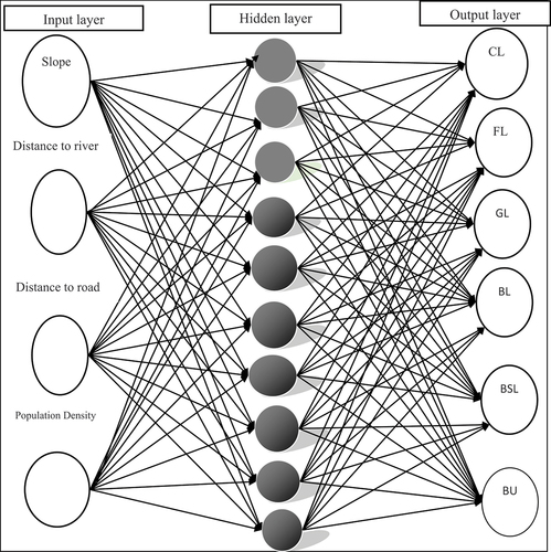
The 2014 and 2020 raster maps were used to model LULC change for the projection year, 2040 (Fig 9). It was employed to generate the transition potential of the LULC dynamic of the target year after considering all possible associations between all input components, and the land use transition was evaluated. The feedforward ANN predicts and classifies land use land cover change using a supervised backpropagation approach. It is made up of three layers: input, hidden, and output, which can detect differences in the input and output patterns. Each neuron generates a value that is the product of the values stored in the nodes of the layer above it and the network weights between them for this procedure. The prediction LULC maps were developed using the dynamics and patterns of existing LULCs.

Figure 9. Predicted LULC change from 2020 to 2040 in the Suha watershed.

The simulated 2020 map was compared to the actual classified 2020 LULC map to validate the CA-ANN-MLP model. The model was trained with a learning rate of 0.001 and momentum of 0.001. The CA-ANN-MLP training process was repeated 100 times with a neighborhood value of 3 pixels and 10 hidden layers. The trained model was then simulated to produce 2040 maps. CA-ANN -MPL is built on interactions between connected neurons and changes in the strength of the connections that support those interactions (Bhartendu et al., 2022).

In general, the plugin and model (CA-ANN-MLP) model generated a transition probability matrix that displays the proportion of classes that have changed to other classes and calculates the rate of the altered area in a given year. It developed a change map from 2014 to 2020 for each of the six LULC classifications in the research area, which are cultivated land, forestland, pasture land, bare land, bush-shrub land, and built-up area. The LULC dynamic of 2040 was estimated based on the dynamics and pattern of the existing LULC (2020-LULC and other specified factors) using raster maps from 2020.

3.10. LULC dynamic and map of the predicted years (2040)

The CA-ANN simulation was used to generate forecasted LULC maps for the study watershed from 2020 to 2040. The total area covered by the six different LULC classes and their areal cover is illustrated in Table 10. The observed outcomes clarified that there is a steady land use land cover changes within the study period. Due to a continued change, bare land has shown the highest and most significant increment from 7075 ha (8.96%) in 2020 to 7103.37 ha (12.55%) in 2040 as compared to the other land use categories. Similarly, the built-up area has shown substantial growth from 7157 ha (9.07%) in 2020 to 7157 ha (9.66) in 2040. Cultivated land was also the other LULC type that exhibited an increment in the prediction where the area increased from 48,025 ha (60.83 %) in 2020 to 48,028 ha (61.21%) in 2040. On the other hand, due to the high increasing rate of bare land and built-up area, the highest diminishing trends were observed in the bush-shrub land from 8001 ha (10.13%) in 2020 to 7976.52 (7.03%) in 2040 which was followed by grazing land 5587 ha (7.08%) in 2020 to 5578.23 ha (5.97%) in 2040 in the change detection matrix. Similarly, forestland experiences a decline from 3106 ha (3.93%) in 2020 to 3103.15 (3.57%) in 2040. A similar research report conducted in Bihar, India, indicated that both are showing continuous increment regarding bare land and built-up area whereas in the case of cultivated land, a decreasing trend was found which is contrary to the finding of this study (Bhartendu et al., 2022). A prediction of LULC study conducted by Girma et al. (2022) in the Gidabo watershed, Ethiopia, indicated that agricultural land, built-up area, and bare land showed the possible expansion over the expense of the other LULC types (forest, grassland, and shrub lands) in the future (2021–2035). Generally, the highest conversion of land in terms of gaining and losing in areal coverage was detected at bare and bush-shrub land by 3.61% and 3.11%, respectively, from 2020 to 2040.

Table 10. The predicted area of the LULC change in hectares in Suha Watershed (2021-2040)

LULC Classes	2020 (ha)	2040 (ha)	Δ(ha)	2020%	2040%	Δ %
Cultivated land	48025	48028	3.00	60.83	61.21	0.38
Forest land	3106	3103.15	−2.85	3.93	3.57	−0.36
Grazing land	5587	5578.23	−8.77	7.08	5.97	−1.11
Bare land	7075	7103.37	28.37	8.96	12.55	3.61
Bush-Shrub land	8001	7976.52	−24.48	10.13	7.03	−3.11
Built up land	7157	7161.73	4.73	9.07	9.66	0.60
Total	78951	78951	789.51	789.51	0	100.00

This suggests that the constantly changing patterns in LULC will have a negative impact on land system processes, particularly the growth in built-up land and the loss of natural vegetation such as forest and bush-shrub land (Bhartendu et al., 2022; Karakuş, 2019). Ethiopia has been facing recurrent drought and flooding every year which touches many parts of the country including the study area (Kidane et al., 2019; Regasa et al., 2021; Tewabe et al., 2020).

3.11. The implication of LULC change on climate variability

Land use/land cover change is inextricably related to local climate patterns in a variety of ways, and it plays an important part in the interaction between the land and the atmosphere (Fan et al., 2015). It has the potential to cause climatic variability/change at a variety of regional and temporal dimensions. Changes in land use/land cover, for example, alter the flow of sensible heat between the land surface and the atmosphere, which influences the local climate through greenhouse gas absorption or emission and by changing the physical qualities of the land surface (Yesuph & Dagnew, 2019). As a result, changes in LULC, such as the conversion of forestland to agricultural land uses, can have a significant impact on land surface climate interactions by modifying the exchange of heat, moisture, trace gas fluxes, and albedo. It can also have a significant impact on evapotranspiration rates, which can enhance climate extremes such as droughts.

In this study, the analysis of NDVI and the major climate elements (LST and rainfall) indicated that there is a strong correlation in the given LULC categories in the study area. In one of the LULC types, the correlation coefficient reached as high as 0.97 (Table 4). As shown above, the impact of LULC change on climate elements can be examined by analyzing the changes in NDVI of each LULC.

The correlation indicates that the LST of the study area increases as the NDVI value of each land use/land cover is reduced in each land use type within the study period (in each decade). For example, the zonal statistic of the NDVI against LST indicated that the mean LST of vegetated area (forestland, grazing land, and bush-shrub lands) is greater than the non-vegetated area (cultivated land, bare land and built-up area) in the area through the study period (1990 to 2020). To see this, the mean NDVI value of relatively vegetated LULC categories were 0.45,0.31, and 0.28, whereas their LST records were 24.89°C, 26.13°C, and 27.58°C in 1990. In the meantime, the mean LST records in the non-vegetated LULC types were 30.89°C, 30.67°C and 28.89°C whereas their mean NDVI were 0.22,0.20 and 0.25 in the same year (1990). Similarly, the non-vegetated area LST is significantly higher than the LST records of vegetated areas in 2020.

The reason behind this is that the NDVI value of the non-vegetated area (cultivated land ,bare land and built up) area considerably decreased from time to time as compared to the vegetated area in the study area. The NDVI values were 0.09, 0.17, and 0.13 and their LST were 28.89°C, 30.89°C, and 30.67°C while the NDVI value of the vegetated area were 0.12, 0.15, and 0.11, and their LST records were 24.89°C, 26.13°C, and 27.58°C, respectively, in the watershed. Furthermore, in both cases, a regression line produced dramatic clarification, showing a strong negative relationship between NDVI and LST. The same investigation on the relationship between LST and NDVI showed that forest/grass environments with high NDVI had much lower LST because high forest cover reduces the heat stored in the soil and surface structures through transpiration, in addition to the shadow impact (Kidane et al., 2019; Mekasha et al., 2022; Tewabe & Fentahun, 2020).

Figure 10. The relationship between mean annual LST and NDVI in the Suha watershed.

However, the correlation between rainfall and NDVI was found to be positive and strong in the study area in general though there is a great variation among each land use type which is similar to the findings of others (Nega et al.,2019).

Finally, the zonal statistics between NDVI and rainfall also show that the vegetated areas have relatively more rainfall than the non-vegetated areas (lesser mean rainfall). For instance, in 1990, the NDVI values of forestland, bush-shrub land, and grazing land were 0.45, 0.30, and 0.38, respectively, whereas the average rainfall records in the same LULCs were 1085.51 mm, 1061.48 mm, and 1053.27 mm. On the other hand, NDVI in the less vegetated areas such as bare land, cultivated land, and built-up area was found as 0.20, 0.22, and 0.25, while the rainfall was 1053.24 mm, 1073.92 mm, and 1085.62 mm, respectively, as shown in Table 8. In the same year, the mean annual rainfall over vegetated and non-vegetated areas was 1,402.7 mm and 1,243 mm, respectively, in the watershed (Figure 11).

The NDVI value of those more vegetated and less vegetated areas was also seen to detect whether the trend between LULCs and rainfall was decreasing in the same direction and extent or not in the watershed in 2020. The result showed that land use/covers such as forest, bush-shrub, and grazing land had higher NDVI value and rainfall than those less LULC categories. It was found that the mean NDVI values of those land use categories were 0.12,0.11, and 0.15, while the rainfall records were 1058.41 mm,1049.58 mm, and 1059.97 mm, respectively, in 2020. Contrary to this, the value of the less vegetated areas such as bare land, built and cultivated lands were 0.17, 0.13, and 0.09, while the mean annual rainfall records were 1004.93 mm, 1044.01 mm, and 1047.04 mm, respectively, in 2020 in the watershed. When the NDVI value of a given LULC decreases, the mean rainfall amount of that land use type also declines by a certain level (Fig. 9). Studies conducted by Kidane et al. (2019) and Nega et al. (2019) also reported that the vegetated areas experienced more rainfall (greater minimum, maximum, and mean) than the non-vegetated areas through time.

Figure 11. The relationship between mean annual rainfall and NDVI in the Suha watershed.

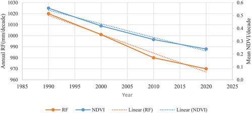
Generally, the results confirmed that the NDVI value with rainfall in the watershed indicated that the mean annual rainfall and NDVI were high in 1990 and low in 2020. This means that NDVI and mean annual rainfall decreased from 1990 to 2020 in the watershed. The regression line in Fig. 11 also supported this finding that at the beginning (1990), both NDVI and rainfall were found at the top. In contrast, at the end (2020), these variables fall to the lower value simultaneously, which implies that both had a strong positive relationship in the study area under the investigation period (1990 to 2020).

4. Conclusion

In this study, Landsat images were used to recover and determine the spatial pattern of LULC and main climate variables (LST and rainfall) in the Suha watershed, a northwest highland of Ethiopia, from 1990 to 2020. In the research area, the variance of LST and rainfall over six different land use/land cover classes were studied over a decadal period. The results of LULC analysis suggested that there was a significant conversion from one type to the other classes in the last three decades in the study area. Compared to other groups of land in the watershed, agricultural land, built-up areas, and bare/crop-out land dominated the conversion process, experiencing a significant increase in size. In addition to the direct assessment, the rapid land use/land cover conversion was traced by using the proxy indicator of the respective land use NDVI values from the study period. The result indicated that the NDVI value of each land use/land cover class was decreasing from time to time. The spatiotemporal distribution of LST and rainfall were also detected from the land sat image and other sources in the watershed over the study period on a decadal basis. The LST showed a drastically increasing trend, while the rainfall revealed a considerably decreasing trend from 1990 to 2020.

Based on the findings, the correlation between the different land use/land cover changes and LST was strong and negative. The relationship between LULC and rainfall, on the other hand, was shown to be reasonably robust and positive in the research area. To determine the impact of land use/land cover change on the primary climatic elements, the coefficient of determination (R²) was calculated using land use/land cover classes as an independent predictor and the climate factors as response variables. The proportion of variance explained by the different land use/land classes in the LST and rainfall variables was substantial in each decadal period in the research area. The variation in mean annual LST explained by LULC was more pronounced than that of rainfall in the study area. This implies that the relationship between LST and LULC was relatively stronger than that of rainfall in the area. The predicted LULC dynamics also indicated that vegetated areas would show a remarkable shrink whereas the cultivated land, bare land, and built-up areas will expand over the expense of the above LULC types, which in turn affect the local climate trends.

Generally, the study clarified that the LULC changes become very rapid from time to time due to the high demand for land and its related resources (forest, grasses, water, etc.) for various purposes, which in turn negatively affect the spatiotemporal distribution pattern of local climates. This would again impose a negative impact on the overall socio-economic productivity of the local communities, particularly on smallholder farmers.

Hence, having compatible strategies and policies that could properly work with the utilization of natural resources (land and its related elements) is an undeniable fact since the impact of LULC conversion over the other essential climate elements such as LST and rainfall is significant in the area.

Disclosure statement

No potential conflict of interest was reported by the author(s).

References

- Amare, Wondie, M., Mekuria, W., & Darr, D. (2018). Agroforestry of smallholder farmers in Ethiopia: Practices and benefits. Small-Scale Forestry, 18(1), 39–24. https://doi.org/10.1007/s11842-018-9405-6
- Asfaw, Simane, B., Hassen, Asfaw, A., Hassen, A., & Bantider, A. (2018). Variability and time series trend analysis of rainfall and temperature in northcentral Ethiopia: A case study in Woleka sub-basin. Weather and Climate Extremes, 19, 29–41. https://doi.org/10.1016/j.wace.2017.12.002
- Assefa, A. (2011). Community based watershed development for climate change adaptation in Choke Mountain: The case of upper muga watershed in East Gojjam of Ethiopia.
- Ayele, G., Hayicho, H., & Alemu, M. (2019). Land use land cover change detection and deforestation modeling: In Delomena district of Bale zone, Ethiopia. Journal of Environmental Protection, 10(4), 532–561. Article 4 https://doi.org/10.4236/jep.2019.104031
- Baig, M. F., Mustafa, M. R. U., Baig, I., Takaijudin, H. B., & Zeshan, M. T. (2022). Assessment of land use land cover changes and future predictions using CA-ANN simulation for Selangor, Malaysia. Water, 14(3). Article 3. https://doi.org/10.3390/w14030402402.
- Belay, & Mengistu, D. A. (2019). Land use and land cover dynamics and drivers in the muga watershed, upper Blue Nile basin, Ethiopia. Remote Sensing Applications: Society & Environment, 15, 100249. https://doi.org/10.1016/j.rsase.2019.100249
- Belay, T., & Mengistu, D. A. (2019). Land use and land cover dynamics and drivers in the muga watershed, upper Blue Nile basin, Ethiopia. Remote Sensing Applications: Society & Environment, 15, 100249. https://doi.org/10.1016/j.rsase.2019.100249
- Belay, T., & Mengistu, D. A. (2021). Impacts of land use/land cover and climate changes on soil erosion in Muga watershed, upper Blue Nile basin (Abay), Ethiopia. Ecological Processes, 10(1), 68. https://doi.org/10.1186/s13717-021-00339-9
- Berhanu, W., & Beyene, F. (2015). Climate variability and household adaptation strategies in Southern Ethiopia. Sustainability, 7(6), 6353–6375. https://doi.org/10.3390/su7066353
- Berhanu, B., & Bisrat, E. (2018). Identification of surface water storing sites using Topographic Wetness Index (TWI) and Normalized Difference Vegetation Index (NDVI). Journal of Natural Resources & Development, 8, 91–100. https://doi.org/10.5027/jnrd.v8i0.09
- Bhartendu, S., Varun, M., Shruti, K., & Gowhar, M. (2022). Cellular automata-based artificial neural network model for assessing past, present, and future land use/land cover dynamics. Agronomy. 12(11):2772
- Chibuike, E. M., Ibukun, A. O., Abbas, A., & Kunda, J. J. (2018). Assessment of green parks cooling effect on Abuja urban microclimate using geospatial techniques. Remote Sensing Applications: Society & Environment, 11, 11–21. https://doi.org/10.1016/j.rsase.2018.04.006
- CSA. (2007). Population and housing census of Ethiopia. Central Statistical Agency (CSA).
- Debie, E., Anteneh, M., & Asmare, T. (2022). Land use/cover changes and surface temperature dynamics over abaminus watershed, Northwest Ethiopia. Air, Soil and Water Research, 15, 11786221221097916. https://doi.org/10.1177/11786221221097917
- Deng, X., Zhao, C., & Yan, H. (2013). Systematic modeling of impacts of land use and land cover changes on regional climate: A review. Advances in Meteorology, 2013, 1–11. https://doi.org/10.1155/2013/317678
- Dibaba, W. T., Demissie, T. A., & Miegel, K. (2020a). Drivers and implications of land use/land cover dynamics in Finchaa catchment, northwestern Ethiopia. Land, 9(4). Article 4. https://doi.org/10.3390/land9040113.
- Dibaba, W. T., Demissie, T. A., & Miegel, K. (2020b). Drivers and implications of land use/land cover dynamics in Finchaa catchment, northwestern Ethiopia. Land, 9(4). Article 4. https://doi.org/10.3390/land9040113.
- Driouech, F., ElRhaz, K., Moufouma-Okia, W., Arjdal, K., & Balhane, S. (2020). Assessing future changes of climate extreme events in the CORDEX-MENA region using regional climate model ALADIN-Climate. Earth Systems and Environment, 4(3), 477–492. https://doi.org/10.1007/s41748-020-00169-3
- Eggen, M., Ozdogan, M., Zaitchik, B., & Simane, B. (2016). Land cover classification in complex and fragmented agricultural landscapes of the Ethiopian highlands. Remote Sensing, 8(12), 1020. https://doi.org/10.3390/rs8121020
- Evans, R. H. (1996). An analysis of Criterion variable reliability in Conjoint analysis. Perceptual and Motor Skills, 82(3), 988–990. https://doi.org/10.2466/pms.1996.82.3.988
- Fan, X., Ma, Z., Yang, Q., Han, Y., & Mahmood, R. (2015). Land use/land cover changes and regional climate over the Loess Plateau during 2001–2009. Part II: Interrelationship from observations. Climatic Change, 129(3), 441–455. https://doi.org/10.1007/s10584-014-1068-5
- Feke, B. E., Terefe, T., Ture, K., & Hunde, D. (2021). Spatiotemporal variability and time series trends of rainfall over northwestern parts of Ethiopia: The case of Horro Guduru Wollega Zone. Environmental Monitoring and Assessment, 193(6), 367. https://doi.org/10.1007/s10661-021-09141-8
- G/Eyesus, Y., Tesfaye, K., Mamo, G., Yeshanew, A., & Bekele, E. (2003). The use of agro climatic zones as a basis for tailored seasonal rainfall forecasts for the cropping systems in the central rift valley of Ethiopia. Insights and Tools for Adaptation: Learning from Climate Variability. https://doi.org/10.13140/2.1.1709.1522
- Girma, R., Fürst, C., & Moges, A. (2022). Land use land cover change modeling by integrating artificial neural network with cellular Automata-Markov chain model in Gidabo river basin, main Ethiopian rift. Environmental Challenges, 6, 100419. https://doi.org/10.1016/j.envc.2021.100419
- Gogoi, P. P., Vinoj, V., Swain, D., Roberts, G., Dash, J., & Tripathy, S. (2019). Land use and land cover change effect on surface temperature over Eastern India. Scientific Reports, 9(1). Article 1. https://doi.org/10.1038/s41598-019-45213-z.
- Gohain, K. J., Mohammad, P., & Goswami, A. (2021). Assessing the impact of land use land cover changes on land surface temperature over Pune city, India. Quaternary International, 575–576, 259–269. https://doi.org/10.1016/j.quaint.2020.04.052
- Guha, S., Govil, H., Taloor, A. K., Gill, N., & Dey, A. (2022). Land surface temperature and spectral indices: A seasonal study of Raipur city. Geodesy and Geodynamics, 13(1), 72–82. https://doi.org/10.1016/j.geog.2021.05.002
- Hageback, J., Sundberg, J., Ostwald, M., Chen, D., Yun, X., & Knutsson, P. (2005). Climate variability and land-use change in Danangou watershed, China—examples of small-scale farmers’ adaptation. Climatic Change, 72(1–2), 189–212. https://doi.org/10.1007/s10584-005-5384-7
- Hajihosseini, M., Hajihosseini, H., Morid, S., Delavar, M., & Booij, M. J. (2019). Impacts of land use changes and climate variability on transboundary Hirmand river using SWAT. Journal of Water and Climate Change, 11(4), 1695–1711. https://doi.org/10.2166/wcc.2019.100
- Hassen, E. E., & Assen, M. (2018). Land use/cover dynamics and its drivers in Gelda catchment, Lake Tana watershed, Ethiopia. Environmental Systems Research, 6(1). Article 1. https://doi.org/10.1186/s40068-017-0081-x.
- Hereher, M. E. (2017). Effect of land use/cover change on land surface temperatures—the Nile Delta, Egypt. Journal of African Earth Sciences, 126, 75–83. https://doi.org/10.1016/j.jafrearsci.2016.11.027
- Hussain, S., & Karuppannan, S. (2021). Land use/land cover changes and their impact on land surface temperature using remote sensing technique in district Khanewal, Punjab Pakistan. Geology, Ecology & Landscapes, 0(1), 46–58. https://doi.org/10.1080/24749508.2021.1923272
- Hussain, S., Lu, L., Mubeen, M., Nasim, W., Karuppannan, S., Fahad, S., Tariq, A., Mousa, B. G., Mumtaz, F., & Aslam, M. (2022). Spatiotemporal variation in land use land cover in the response to local climate change using multispectral remote sensing data. Land, 11(5), 595. Article 5 https://doi.org/10.3390/land11050595
- Hussien, K., Kebede, A., Mekuriaw, A., Asfaw Beza, S., & Haile Erena, S. (2023). Modelling spatiotemporal trends of land use land cover dynamics in the Abbay river basin, Ethiopia. Modeling Earth Systems and Environment, 9(1), 347–376. https://doi.org/10.1007/s40808-022-01487-3
- John, J., Bindu, G., Srimuruganandam, B., Wadhwa, A., & Rajan, P. (2020). Land use/land cover and land surface temperature analysis in Wayanad district, India, using satellite imagery. Annals of GIS, 26(4), 343–360. https://doi.org/10.1080/19475683.2020.1733662
- Karakuş, C. B. (2019). The impact of Land Use/Land Cover (LULC) changes on land surface temperature in Sivas city center and its surroundings and Assessment of urban heat island. Asia-Pacific Journal of Atmospheric Sciences, 55(4), 669–684. https://doi.org/10.1007/s13143-019-00109-w
- Kebede, A. S. (2018). Assessment of land use/land cover change using GIS and remote sensing techniques: A case study of Dendi district, Oromiya regional State. Undefined./paper/Assessment-of-Land-Use%2F-Land-Cover-Change-Using-GIS-Kebede/34450d65c2eab39c488e9275c8633868aa934686.
- Khun, L. Y., Amnat, C., Atsamon, L., Pariwate, V., & Can Trong, N. (2021). Land use land cover changes and their effects on surface Air temperature in Myanmar and Thailand.
- Kidane, M., Tolessa, T., Bezie, A., Kessete, N., & Endrias, M. (2019). Evaluating the impacts of climate and Land Use/Land Cover (LU/LC) dynamics on the hydrological responses of the upper Blue Nile in the central highlands of Ethiopia. Spatial Information Research, 27(2), 151–167. https://doi.org/10.1007/s41324-018-0222-y
- Kindu, M., Schneider, T., Teketay, D., & Knoke, T. . (2013). Land Use/Land Cover Change Analysis Using Object-Based Classification Approach in Munessa-Shashemene Landscape of the Ethiopian highlands. Remote Sensing, 5(5). https://doi.org/10.3390/rs5052411.
- Laux, P., Nguyen, P. N. B., Cullmann, J., & Kunstmann, H. (2017). Impacts of land-use/Land-cover change and climate change on the regional climate in the central Vietnam. In A. Nauditt & L. Ribbe (Eds.), Land use and climate change interactions in central Vietnam (pp. 143–151). Springer Singapore. https://doi.org/10.1007/978-981-10-2624-9_9
- Leta, M. K., Demissie, T. A., & Tränckner, J. (2021). Modeling and prediction of land use land cover change dynamics based on Land Change Modeler (LCM) in nashe watershed, upper Blue Nile basin, Ethiopia. Sustainability, 13(7), 3740. Article 7 https://doi.org/10.3390/su13073740
- Li, J., Lewis, J., Rowland, J., Tappan, G., & Tieszen, L. L. (2004). Evaluation of land performance in Senegal using multi-temporal NDVI and rainfall series. Journal of Arid Environments, 59(3), 463–480. https://doi.org/10.1016/j.jaridenv.2004.03.019
- Madariya, G., & Sharma, S. P. D. S. (2022). A comparative study on supervised and unsupervised techniques of land use and land cover classification.
- Mekasha, S. T., Suryabhagavan, K. V., & Kassawmar, T. (2022). Geospatial modeling of forest cover dynamics and impact on climate variability in Awi zone, Ethiopia. Tropical Ecology, 63(2), 183–199. https://doi.org/10.1007/s42965-021-00199-6
- Mekuriaw, A., Cherinet, M., & Tsegaye, L. (2020). Assessing the impact of land cover changes on selected ecosystem services in upper Suha watershed, Gojjam, Ethiopia. International Journal of River Basin Management, 19(4), 459–467. https://doi.org/10.1080/15715124.2019.1704767
- Merga, B. B., Moisa, M. B., Negash, D. A., Ahmed, Z., & Gemeda, D. O. (2022). Land surface temperature variation in response to land-use and land-cover dynamics: A case of Didessa river sub-basin in Western Ethiopia. Earth Systems and Environment, 6(4), 803–815. https://doi.org/10.1007/s41748-022-00303-3
- Minale, A. S., & Rao, K. K. (2012). Impacts of land cover/use dynamics of Gilgel Abbay catchment of Lake Tana on climate variability, northwestern Ethiopia. Applied Geomatics, 4(3), 155–162. https://doi.org/10.1007/s12518-012-0092-2
- Mngube, F. M., Kapiyo, R., Aboum, P., Anyona, D., & Dida, G. O. (2020). Subtle Impacts of temperature and rainfall patterns on land cover change overtime and future projections in the Mara river basin, Kenya. Open Journal of Soil Science, 10(9), 327–358. Article 9 https://doi.org/10.4236/ojss.2020.109018
- Mohammed, G. H., Colombo, R., Middleton, E. M., Rascher, U., van der Tol, C., Nedbal, L., Goulas, Y., Pérez-Priego, O., Damm, A., Meroni, M., Joiner, J., Cogliati, S., Verhoef, W., Malenovský, Z., Gastellu-Etchegorry, J.-P., Miller, J. R., Guanter, L., Moreno, J., Moya, I., & Zarco-Tejada, P. J. (2019). Remote sensing of solar-induced chlorophyll fluorescence (SIF) in vegetation: 50 years of progress. Remote Sensing of Environment, 231, 111177. https://doi.org/10.1016/j.rse.2019.04.030
- Nayak, S. (2021). Land use and land cover change and their impact on temperature over central India. Letters in Spatial and Resource Sciences, 14(2), 129–140. https://doi.org/10.1007/s12076-021-00269-2
- Nega, W., Hailu, B. T., & Fetene, A. (2019). An assessment of the vegetation cover change impact on rainfall and land surface temperature using remote sensing in a subtropical climate, Ethiopia. Remote Sensing Applications: Society & Environment, 16, 100266. https://doi.org/10.1016/j.rsase.2019.100266
- Regasa, M. S., Nones, M., & Adeba, D. (2021). A review on land use and land cover change in Ethiopian basins. Land, 10(6), 585. https://doi.org/10.3390/land10060585
- Rwanga, S., & Ndambuki, J. (2017). Accuracy Assessment of land use/land cover classification using remote sensing and GIS. International Journal of Geosciences, 08(4), 611–622. https://doi.org/10.4236/ijg.2017.84033
- Schmidt, M., Klein, D., Conrad, C., Dech, S., & Paeth, H. (2013). On the relationship between vegetation and climate in tropical and northern Africa. Theoretical and Applied Climatology, 115(1–2), 341–353. https://doi.org/10.1007/s00704-013-0900-6
- Sewnet, A. (2015). Land use/cover change at Infraz watershed, Northwestren Ethiopia. Journal of Landscape Ecology, 8(1), 69–83. Article 1 https://doi.org/10.1515/jlecol-2015-0005
- Sleeter, B., Loveland, T. R., Domke, G. M., Herold, N., Wickham, J., & Wood, N. J. (2018). Chapter 5: Land cover and land use change. In Impacts, risks, and adaptation in the United States: The fourth national climate assessment, volume II. U.S. Global Change Research Program. https://doi.org/10.7930/NCA4.2018.CH5
- Tan, J., Yu, D., Li, Q., Tan, X., & Zhou, W. (2020). Spatial relationship between land-use/land-cover change and land surface temperature in the Dongting Lake area, China. Scientific Reports, 10(1). Article 1. https://doi.org/10.1038/s41598-020-66168-6.
- Tewabe, D., Fentahun, T., & Li, F. (2020). Assessing land use and land cover change detection using remote sensing in the Lake Tana basin, northwest Ethiopia. Cogent Environmental Science, 6(1), 1778998. https://doi.org/10.1080/23311843.2020.1778998
- Traore, M., Lee, M. S., Rasul, A., & Balew, A. (2021). Assessment of land use/land cover changes and their impacts on land surface temperature in Bangui (the capital of Central African Republic). Environmental Challenges, 4, 100114. https://doi.org/10.1016/j.envc.2021.100114
- Tsidu, G. M. (2012). High-resolution monthly rainfall database for Ethiopia: Homogenization, reconstruction, and Gridding. Journal of Climate, 25(24), 8422–8443. https://doi.org/10.1175/JCLI-D-12-00027.1
- USGS. (2019). Landsat 8 Data Users Handbook | U.S. Geological Survey. https://www.usgs.gov/media/files/landsat-8-data-users-handbook
- WoldeYohannes, A., Cotter, M., Kelboro, G., & Dessalegn, W. (2018). Land use and land cover changes and their effects on the landscape of Abaya-Chamo basin, Southern Ethiopia. Land, 7(1), 2. Article 1 https://doi.org/10.3390/land7010002
- Xiao, H., & Weng, Q. (2007). The impact of land use and land cover changes on land surface temperature in a karst area of China. Journal of Environmental Management, 85(1), 245–257. https://doi.org/10.1016/j.jenvman.2006.07.016
- Yeneneh, N., Elias, E., & Legese, G. (2022). Detection of land use/land cover and land surface temperature change in the Suha watershed, North-Western highlands of Ethiopia. Environmental Challenges, 7, 13. https://doi.org/10.1016/j.envc.2022.100523
- Yesuph, A. Y., & Dagnew, A. B. (2019). Land use/cover spatiotemporal dynamics, driving forces and implications at the beshillo catchment of the Blue Nile basin, North Eastern highlands of Ethiopia. Environmental Systems Research, 8(1), 21. https://doi.org/10.1186/s40068-019-0148-y
- Yin, J., He, F., Xiong, Y. J., & Qiu, G. Y. (2017). Effects of land use/land cover and climate changes on surface runoff in a semi-humid and semi-arid transition zone in northwest China. Hydrology and Earth System Sciences, 21(1), 183–196. https://doi.org/10.5194/hess-21-183-2017
- Yue, W., Xu, J., Tan, W., & Xu, L. (2007). The relationship between land surface temperature and NDVI with remote sensing: Application to Shanghai Landsat 7 ETM+ data. International Journal of Remote Sensing, 28(15), 3205–3226. https://doi.org/10.1080/01431160500306906
- Zhang, Y., & Liang, C. (2020). Analysis of annual and seasonal precipitation variation in the Qinba Mountain area, China. Scientific Reports, 10(1), 961. https://doi.org/10.1038/s41598-020-57743-y