Bayesian estimation to identify crystalline phase structures for X-ray diffraction pattern analysis

ABSTRACT

Crystalline phase structure is essential for understanding the performance and properties of a material. Therefore, this study identified and quantified the crystalline phase structure of a sample based on the diffraction pattern observed when the crystalline sample was irradiated with electromagnetic waves such as X-rays. Conventional analysis necessitates experienced and knowledgeable researchers to shorten the list from many candidate crystalline phase structures. However, the Conventional diffraction pattern analysis is highly analyst-dependent and not objective. Additionally, there is no established method for discussing the confidence intervals of the analysis results. Thus, this study aimed to establish a method for automatically inferring crystalline phase structures from diffraction patterns using Bayesian inference. Our method successfully identified true crystalline phase structures with a high probability from 50 candidate crystalline phase structures. Further, the mixing ratios of selected crystalline phase structures were estimated with a high degree of accuracy. This study provided reasonable results for well-crystallized samples that clearly identified the crystalline phase structures.

GRAPHICAL ABSTRACT

IMPACT STATEMENT

We developed a method to automatically estimate crystalline phase structures from diffraction patterns using Bayesian inference. Our method successfully identified true crystalline phase structures with a high probability from 50 candidate crystalline phase structures.

KEYWORDS:

• X-ray diffraction
• Bayesian inference
• model selection
• automatic spectral analysis
• replica exchange Monte Carlo method

1. Introduction

Crystalline phase structure is essential for understanding the performance and properties of a material. Therefore, this study identified and quantified the crystalline phase structure of a sample based on the diffraction pattern observed when the crystalline sample was irradiated with electromagnetic waves such as X-rays. The measurement of the diffraction patterns using X-rays as probes is known as X-ray diffraction (XRD). The crystal structure of a material can be understood by analyzing the diffraction peaks in the XRD data.

A typical XRD data analysis method involves a simple comparison of the measured XRD data with a database. This method first detects the diffraction peaks in the measured XRD data by the smoothed derivative [1–3]. Thereafter, the diffraction angles of the detected peaks are compared with those of the diffraction patterns registered in the database and the similarity to the diffraction patterns in the database is calculated. The diffraction patterns ranked by similarity are suggested by an analyst. Thus, in a typical analysis, the experience and knowledge of the researcher are crucial to shorten the list from several candidate crystal structures. However, the typical diffraction pattern analysis is highly analyst-dependent and not objective. Additionally, there is no established method for discussing the confidence intervals of the analysis results. Consequently, the interpretation of the analysis results is highly dependent on the analysts. Diffraction pattern analysis methods have been proposed to solve such analytical problems [4,5].

In recent years, methods for diffraction-pattern analysis using Bayesian estimation have been proposed, allowing confidence intervals to be discussed [6,7]. Mikhalychev proposed a method for naive Bayesian estimation of crystalline phase structure using a simple model with intensity information only, without considering the peak profile, the background, and the Poisson noise model [7]. In addition, black-box optimization methods have been proposed for hyperparameters that are subjectively determined by an analyst [8]. The proposed method is effective for solving several problems in diffraction pattern analyses. However, this has not been sufficiently discussed from the perspective of automatic estimation of the crystal structure contained in a measured sample from the diffraction pattern. Identifying the crystalline phase structures contained in a diffraction pattern is challenging because the number of candidate crystalline phase structures can be in the order of tens or hundreds, leading to combination explosions. Moreover, this problem requires considerable computational time because the crystal structure contains dozens of diffraction peaks. Despite these challenges, it is necessary to establish a method for identifying crystalline phase structures from diffraction patterns with confidence intervals (probability).

This study aimed to establish a method for the automatic estimation of crystalline phase structures from diffraction patterns. The proposed method decomposes the measured diffraction patterns and automatically selects crystalline phase structures using the diffraction patterns measured at each institute associated with the crystal structures or obtained via simulations as basis functions. The proposed method makes three main contributions to literature.

• Crystalline phase structures can be selected precisely and automatically.

• Posterior distributions can be estimated (confidence intervals can be discussed).

• A global solution is provided (no initial value dependence).

The proposed method, which extracts material descriptors corresponding to the crystal structure from measured diffraction patterns, is expected to play an important role in promoting the development of data-driven materials. Note that in this paper the term ‘crystal structure’ refers specifically to the crystalline phase structure.

In this study, we provide reasonable results that allow clearer identification of the crystalline phase structures for more crystalline structures. Surprisingly, our method successfully detected crystalline phase structures containing only 2 [%]. However, a crystalline phase structure that contained only 1 [%] of the sample could not be detected, although we proposed a similar crystalline phase structure with low probability, suggesting a reasonable result.

2. Concept

Figure 1 shows an observation process of XRD data and a conceptual diagram of the proposed method. We suppose a multitude of candidate crystal phases and structures $\mathcal{F}$ when preparing the materials. The crystal structures contained in the material are selected by material synthesis, manufacturing processes, etc. This study treats the control variable dealing with crystal structure selection as the indicator variable $\mathit{g}\in \{0,1\}$. Ideally, the crystalline materials produced should have diffraction line spectra corresponding to the crystal phases and structures they contain. In practice, we observe diffraction peaks whose shapes are dependent on the profile parameters $\mathbf{\Theta }$ that correspond to the measurement environment. We considered a situation wherein only the observed diffraction data $\mathcal{D}$ and candidate crystal structures $\mathcal{F}$ were provided.

Figure 1. Observation process of XRD data and a conceptual diagram of the proposed method, that is, Bayesian inverse estimation to identify the crystalline phase structure and their known structures for XRD analysis [9].

The purpose of this study is to develop an automated Bayesian XRD analysis linked a database. In advanced materials, the crystalline phase structure contained in the XRD data is often unknown. This requires a method to automatically identify the crystalline phase structures in the data from a huge number of crystal phase structures in databases. We have therefore developed a methodology to precisely estimate the crystalline phase structure from XRD data by using the Bayesian estimation. In this study, we aimed to inversely estimate the structural indicator $\mathit{g}$ and profile parameter set $\mathbf{\Theta }$ from the observed diffraction data (XRD data) shown in Figure 1. The proposed method is a Bayesian inverse estimation method used to identify crystal structures for XRD analysis.

3. Model

3.1. Problem setting

The purpose is to estimate the profile parameters and the crystalline phase structures in the measured sample, considering the measured XRD data $\mathcal{D}=\{(x_i,y_i){\}}_{\mathit{i}=1}^N$ and the candidate crystal structure $\mathcal{F}$. Here, $x_i\in (0,180)$ and $y_i\in \mathbb{N}$ denote the diffraction angle $2\mathit{\theta }$ [${ }^{\circ }$] and the diffraction intensity [counts], respectively.

The candidate crystal structure factor set $\mathcal{F}$ is expressed as:

(1) $\mathcal{F}=\{{\mathcal{F}}_k|\mathit{k}\in \{1,2,\dots ,\mathit{K}\}\},$(1)

(2) $\mathrm{where}{\mathcal{F}}_k=\{(p_m^{(\mathit{k})},I_m^{(\mathit{k})})|\mathit{m}\in \{1,2,\dots ,M_k\}\}\subset \mathcal{F},$(2)

where $\mathit{K}\in \mathbb{N}$ is the number of candidate crystal structures and ${\mathcal{F}}_k$ is the $\mathit{k}$-th crystal structure factor. The elements of the crystal structure factor $p_m^{(\mathit{k})}\in (0,180)$ and $I_m^{(\mathit{k})}\in [0,1]$ are the diffraction angle (peak position) [${ }^{\circ }$] and relative intensity of the $\mathit{m}$-th diffraction peak in ${\mathcal{F}}_k$ for a crystal structure $\mathit{k}$. Further, $M_k\in \mathbb{N}$ denotes the number of peaks in ${\mathcal{F}}_k$. In this study, the candidate crystal structure factor set $\mathcal{F}$ is provided.

3.2. Profile function

XRD data can be represented by a profile function $f_{\mathcal{F}}(x_i;\mathrm{\Theta }):\mathbb{R}\to {\mathbb{R}}_0^{+}$, which is a linear sum of the signal spectrum $S_{\mathcal{F}}(x_i;{\mathrm{\Theta }}_{\mathrm{S}})$ and the background $\mathit{B}(x_i;{\mathrm{\Theta }}_{\mathrm{B}})$:

(3) $y_i\approx f_{\mathcal{F}}(x_i;\mathrm{\Theta }),$(3)

(4) $=S_{\mathcal{F}}(x_i;{\mathrm{\Theta }}_{\mathrm{S}})+\mathit{B}(x_i;{\mathrm{\Theta }}_{\mathrm{B}}),$(4)

where $(x_i,y_i)$ denote the measured data points, the function $S_{\mathcal{F}}(x_i;{\mathrm{\Theta }}_{\mathrm{S}})$ denotes the signal spectrum based on the candidate crystal structures $\mathcal{F}$, and the function $\mathit{B}(x_i;{\mathrm{\Theta }}_{\mathrm{B}})$ denotes the background. We set $\mathrm{\Theta }=\{{\mathrm{\Theta }}_{\mathrm{S}},{\mathrm{\Theta }}_{\mathrm{B}}\}$ as the profile parameter set. In addition, the sets ${\mathrm{\Theta }}_{\mathrm{S}}$ and ${\mathrm{\Theta }}_{\mathrm{B}}$ are the signal spectrum and background parameter sets, respectively.

The signal spectrum $S_{\mathcal{F}}(x_i;{\mathrm{\Theta }}_{\mathrm{S}})$ is expressed as a linear sum of the profile function (peaks) $C_{{\mathcal{F}}_k}(x_i;{\mathrm{\Theta }}_{\mathrm{S}}^{(\mathit{k})}):\mathbb{R}\to {\mathbb{R}}_0^{+}$ in a crystal structure ${\mathcal{F}}_k$ among the several candidates [10]:

(5) $S_{\mathcal{F}}(x_i;{\mathrm{\Theta }}_{\mathrm{S}})=\sum _{\mathit{k}=1}^K{h}_k{C}_{{\mathcal{F}}_k}(x_i;{\mathrm{\Theta }}_{\mathrm{S}}^{(\mathit{k})}),$(5)

where $h_k\in {\mathbb{R}}^{+}$ denotes the signal intensity of crystal structure factor ${\mathcal{F}}_k$. The profile function $C_{{\mathcal{F}}_k}(x_i;{\mathrm{\Theta }}_{\mathrm{S}}^{(\mathit{k})})$ of candidate crystal structure $\mathit{k}$ is defined as follows:

(6) $C_{{\mathcal{F}}_k}(x_i;{\mathrm{\Theta }}_{\mathrm{S}}^{(\mathit{k})})=\sum _{\mathit{m}=1}^{M_k}{I}_m^{(\mathit{k})}\mathit{V}\left(x_i;{\rho }_{\mathit{mk}},{\mathrm{\Sigma }}_k,{\mathrm{\Omega }}_k,r_k\right),$(6)

(7) $=\sum _{\mathit{m}=1}^{M_k}{I}_m^{(\mathit{k})}\{(1-r_k)\mathit{G}(x_i;{\rho }_{\mathit{mk}},{\mathrm{\Sigma }}_k)+r_k\mathit{L}(x_i;{\rho }_{\mathit{mk}},{\mathrm{\Omega }}_k)\},$(7)

(8) $\mathrm{where}{\rho }_{\mathit{mk}}=p_m^{(\mathit{k})}+{\mu }_k,$(8)

where ${\mu }_k\in \mathbb{R}\mathit{and}{r}_k\in [0,1]$ are the peak shift and Gauss-Lorentz ratio at the peak of crystal structure $\mathit{k}$, respectively, ${\rho }_{\mathit{mk}}\in \mathbb{R}$ is the peak position of the peak function, and the function $\mathit{V}(x_i):\mathbb{R}\to {\mathbb{R}}_0^{+}$ is a pseudo-Voigt function [11]. In addition, $\mathit{G}(x_i):\mathbb{R}\to {\mathbb{R}}_0^{+}$ and $\mathit{L}(x_i):\mathbb{R}\to {\mathbb{R}}_0^{+}$ are Gaussian and Lorentz functions, respectively. ${\mathrm{\Sigma }}_k=\mathrm{\Sigma }(x_i;u_k,v_k,w_k,{\alpha }_k):(0,180)\to {\mathbb{R}}^{+}$ and ${\mathrm{\Omega }}_k=\mathrm{\Omega }(x_i;s_k,t_k,{\alpha }_k):(0,180)\to {\mathbb{R}}^{+}$ are the Gaussian and Lorentzian widths of the peak, respectively, as a function of the diffraction angle $x_i\in (0,180)$. The width functions ${\mathrm{\Sigma }}_k(x_i)$ and ${\mathrm{\Omega }}_k(x_i)$ are expressed as

(9) $\mathrm{\Sigma }(x_i;u_k,v_k,w_k,{\alpha }_k)=\mathit{A}(x_i;{\alpha }_k)\sqrt{u_k{tan}^2\left(\frac{x_i}{2}\right)-v_{k}tan\left(\frac{x_i}{2}\right)+w_k},$(9)

(10) $\mathrm{\Omega }(x_i;s_k,t_k,{\alpha }_k)=\mathit{A}(x_i;{\alpha }_k)\left\{s_{k}sec\left(\frac{x_i}{2}\right)+t_{k}tan\left(\frac{x_i}{2}\right)\right\},$(10)

(11) $\mathrm{where}\mathit{A}(x_i;{\alpha }_k)=\left\{\begin{array}{cc}{\alpha }_k& (x_i\ge {\rho }_k)\\ 1& (x_i<{\rho }_k),\end{array}\right.$(11)

(12) $=\mathit{sign}(x_i-{\rho }_k)\frac{{\alpha }_k-1}{2}+\frac{{\alpha }_k+1}{2},$(12)

where $\{u_k,v_k,w_k\}$ and $\{s_k,t_k\}$ are the Gaussian and Lorentzian width parameter sets, respectively. Function $\mathit{A}(x_i;{\alpha }_k):\mathbb{R}\to \mathbb{R}$ is a function expressing the peak asymmetry, and ${\alpha }_k\in {\mathbb{R}}^{+}$ is the asymmetry parameter for the peak function. Further, the function $\mathrm{sign}(\cdot ):\mathbb{R}\to \{-1,1\}$ is the sign function and the trigonometric function $sec(\mathit{x})$ is $sec(\mathit{x})=1/cos(\mathit{x})$.

The optimization parameter set for the signal spectrum $S_{\mathcal{F}}(x_i;{\mathrm{\Theta }}_{\mathrm{S}})$ is expressed as:

${\mathrm{\Theta }}_{\mathrm{S}}=\{{\mathrm{\Theta }}_{\mathrm{S}}^{(\mathit{k})}|\mathit{k}\in \{1,2,\dots ,\mathit{K}\}\},$

$\mathrm{where}{\mathrm{\Theta }}_{\mathrm{S}}^{(\mathit{k})}=\{(h_k,{\mu }_k,{\alpha }_k,r_k,u_k,v_k,w_k,s_k,t_k)\}.$

Background $\mathit{B}(x_i;{\mathrm{\Theta }}_{\mathrm{B}}):\mathbb{R}\to \mathbb{R}$ is defined as follows:

(13) $\mathit{B}(x_i;{\mathrm{\Theta }}_{\mathrm{B}})=\mathit{aV}(x_i;0.0,{\sigma }_{\mathrm{bg}},{\sigma }_{\mathrm{bg}},r_{\mathrm{bg}})+\mathit{b},$(13)

where the background parameter set is ${\mathrm{\Theta }}_{\mathrm{B}}=\{\mathit{a},{\sigma }_{\mathrm{bg}},r_{\mathrm{bg}},\mathit{b}\}$.

3.3. Generation model

We assume that the observed data $\{(\mathit{Y},\mathit{X})\}=\{(x_i,y_i){\}}_{\mathit{i}=0}^N$ are stochastically distributed owing to statistical noise in the measurement. Next, we consider the joint distribution $\mathit{P}(\mathit{Y},\mathrm{\Theta })$, which can be expanded to $\mathit{P}(\mathit{Y},\mathrm{\Theta })=\mathit{P}(\mathrm{\Theta }|\mathit{Y})\mathit{P}(\mathit{Y})$. Using Bayes’ theorem to swap the orders of $\mathit{Y}$ and $\mathrm{\Theta }$, we can expand $\mathit{P}(\mathit{Y},\mathrm{\Theta })=\mathit{P}(\mathit{Y}|\mathrm{\Theta })\mathit{P}(\mathrm{\Theta })$. Hence, the posterior distribution $\mathit{P}(\mathrm{\Theta }|\mathit{Y})$ is expressed as:

(14) $\mathit{P}(\mathrm{\Theta }|\mathit{Y})=\frac{\mathit{P}(\mathit{Y}|\mathrm{\Theta })P(\mathrm{\Theta })}{\mathit{P}(\mathit{Y})}\propto \mathit{P}(\mathit{Y}|\mathrm{\Theta })\mathit{P}(\mathrm{\Theta }),$(14)

where $\mathit{P}(\mathrm{\Theta }|\mathit{Y})$ and $\mathit{P}(\mathrm{\Theta })$ are the posterior and prior distributions, respectively, in the Bayesian inference. Further, $\mathit{P}(\mathit{Y}|\mathrm{\Theta })$ is the conditional probability of $\mathit{Y}$ given the model parameter set $\mathrm{\Theta }$, which is a probability distribution explained by error theory.

To derive $\mathit{P}(\mathit{Y}|\mathrm{\Theta })$, we consider the observation process of $\{(x_i,y_i)\}$ at the observation data points. Assuming that the observed data are independent of each other, the conditional probability of the observed data $\{(\mathit{Y},\mathit{X})\}$ can be expressed as:

(15) $\mathit{P}(\mathit{Y}|\mathrm{\Theta })=\prod _{\mathit{i}=0}^N\mathit{P}(y_i|\mathrm{\Theta }).$(15)

As XRD spectra are count data, the conditional probability $\mathit{P}(y_i|\mathrm{\Theta })$ of the intensity $y_i$ for the diffraction angle $x_i$ follows a Poisson distribution $\mathcal{P}(y_i|f_{\mathcal{F}}(x_i;\mathrm{\Theta }))$:

(16) $\mathit{P}(y_i|\mathrm{\Theta })=\mathcal{P}(y_i|f_{\mathcal{F}}(x_i;\mathrm{\Theta }))$(16)

(17) $=\frac{{\mathit{f}}_{\mathcal{F}}{(x_i;\mathrm{\Theta })}^{y_i}exp(-f_{\mathcal{F}}(x_i;\mathrm{\Theta }))}{y_i!}.$(17)

The cost function $\mathit{E}(\mathrm{\Theta })\in \mathbb{R}$ is defined by the negative log-likelihood function $\mathit{E}(\mathrm{\Theta })=-ln\mathit{P}(\mathit{Y}|\mathrm{\Theta })$ and is expressed as follows:

(18) $\mathit{E}(\mathrm{\Theta })=-\sum _{\mathit{i}=0}^{N}ln\mathit{P}(y_i|\mathrm{\Theta }),$(18)

(19) $=-\sum _{\mathit{i}=0}^N\left\{y_{i}ln{f}_{\mathcal{F}}(x_i;\mathrm{\Theta })-f_{\mathcal{F}}(x_i;\mathrm{\Theta })-ln{y}_i!\right\}.$(19)

Further, $\mathit{P}(\mathrm{\Theta }|\mathit{Y})$ is expressed using the cost function $\mathit{E}(\mathrm{\Theta })$ and the prior distribution $\mathit{P}(\mathrm{\Theta })$ as follows:

(20) $\mathit{P}(\mathrm{\Theta }|\mathit{Y})\propto \mathit{P}(\mathit{Y}|\mathrm{\Theta })\mathit{P}(\mathrm{\Theta }),$(20)

(21) $=exp\{ln\mathit{P}(\mathit{Y}|\mathrm{\Theta })\}\mathit{P}(\mathrm{\Theta }),$(21)

(22) $=exp\{-\mathit{E}(\mathrm{\Theta })\}\mathit{P}(\mathrm{\Theta }).$(22)

3.4. Identification of crystalline phase structures

In the analysis of XRD spectra, the crystal structure contained in the measured sample is often unknown. Therefore, it is important to accurately estimate the true crystal structure contained in the candidate crystal structures $\mathcal{F}$. We introduce an indicator vector $\mathit{g}=\{g_k\in \{0,1\}|\mathit{k}\in \{1,2,\dots ,\mathit{K}\}\}$, which controls the existence of the crystal structure factors in Equation (5)(5) $S_{\mathcal{F}}(x_i;{\mathrm{\Theta }}_{\mathrm{S}})=\sum _{\mathit{k}=1}^K{h}_k{C}_{{\mathcal{F}}_k}(x_i;{\mathrm{\Theta }}_{\mathrm{S}}^{(\mathit{k})}),$(5) :

(23) $f_{\mathcal{F}}(x_i;\mathit{g},\mathrm{\Theta })=S_{\mathcal{F}}(x_i;\mathit{g},{\mathrm{\Theta }}_{\mathrm{S}})+\mathit{B}(x_i;{\mathrm{\Theta }}_{\mathrm{B}}),$(23)

(24) $S_{\mathcal{F}}(x_i;\mathit{g},{\mathrm{\Theta }}_{\mathrm{S}})=\sum _{\mathit{k}=1}^K{\mathit{g}}_k{h}_k{C}_{{\mathcal{F}}_k}(x_i;{\mathrm{\Theta }}_{\mathrm{S}}^{(\mathit{k})}),$(24)

where ${\mathit{g}}_{-}\mathit{k}=1$ indicates that the crystal structure factor ${\mathcal{F}}_k$ is present in the sample. Conversely, ${\mathit{g}}_{-}\mathit{k}=0$ implies that it is absent.

We now consider the joint distribution $\mathit{P}(\mathit{g},\mathit{Y},\mathit{\theta })$. $\mathit{P}(\mathit{g},\mathit{Y},\mathit{\theta })$ can be expanded to $\mathit{P}(\mathit{g},\mathit{Y},\mathit{\theta })=\mathit{P}(\mathit{Y}|\mathit{g},\mathrm{\Theta })\mathit{P}(\mathit{g})\mathit{P}(\mathrm{\Theta })$. According to Bayes’ theorem, the posterior distribution $\mathit{P}(\mathit{g},\mathrm{\Theta }|\mathit{Y})$ is expressed as:

(25) $\mathit{P}(\mathit{g},\mathrm{\Theta }|\mathit{Y})\propto \mathit{P}(\mathit{Y}|\mathit{g},\mathrm{\Theta })\mathit{P}(\mathit{g})\mathit{P}(\mathrm{\Theta }),$(25)

(26) $=exp(-\mathit{E}(\mathit{g},\mathrm{\Theta }))\mathit{P}(\mathit{g})\mathit{P}(\mathrm{\Theta }).$(26)

The cost function $\mathit{E}(\mathit{g},\mathrm{\Theta })$ that introduces the indicator vector $\mathit{g}$ is expressed as:

(27) $\mathit{E}(\mathit{g},\mathrm{\Theta })=-\sum _{\mathit{i}=0}^{N}ln\mathit{P}(y_i|\mathit{g},\mathrm{\Theta }),$(27)

(28) $=-\sum _{\mathit{i}=0}^N\left\{y_{i}ln{f}_{\mathcal{F}}(x_i;\mathit{g},\mathrm{\Theta })-f_{\mathcal{F}}(x_i;\mathit{g},\mathrm{\Theta })-ln{y}_i!\right\}.$(28)

Using the joint distribution presented above, the indicator vector $\mathit{g}$ is estimated from the marginal posterior distribution as follows:

(29) $\mathit{P}(\mathit{g}|\mathit{Y})=\int \mathit{d}\mathrm{\Theta P}(\mathit{g},\mathrm{\Theta }|\mathit{Y}),$(29)

(30) $=\mathit{P}(\mathit{g})\int \mathit{d}\mathrm{\Theta }exp(-\mathit{E}(\mathit{g},\mathrm{\Theta }))\mathit{P}(\mathrm{\Theta }),$(30)

We estimate the profile and background parameters using the posterior distribution $\mathit{P}(\mathrm{\Theta }|\mathit{Y},\mathit{g})$ on parameter set $\mathrm{\Theta }$.

4. Algorithm

4.1. Replica exchange monte carlo method — REMC method

We perform posterior visualization and the maximum a posteriori (MAP) estimation through sampling from the posterior distribution. A popular sampling method is the Monte Carlo (MC) method, which may be bounded by local solutions for cases when the initial value is affected or the cost function landscape is complex.

Therefore, the replica exchange Monte Carlo (REMC) method [12,13] was used to estimate the global solution. For sampling using the REMC method, a replica was prepared with the inverse temperature $\mathit{\beta }$ introduced as follows:

(31) $\mathit{P}(\mathit{g},\mathrm{\Theta }|\mathit{Y};\mathit{\beta }={\beta }_{\tau })=exp(-{\beta }_{\tau }\mathit{E}(\mathit{g},\mathrm{\Theta }))\mathit{P}(\mathit{g})\mathit{P}(\mathrm{\Theta }),$(31)

where the inverse temperature $\mathit{\beta }$ is $0={\beta }_1<{\beta }_2<\cdots <{\beta }_{\tau }<{\beta }_T=1$. For each replica, the parameters were sampled using the Monte Carlo method.

5. Technique

5.1. Tricks for high speeds

This sub-section describes the techniques used to realize Bayesian inference of XRD spectra. In XRD spectral analysis, the number of candidate crystal structure factors $\{{\mathcal{F}}_k{\}}_{\mathit{k}=1}^K$ and the number of peaks $M_k$ for each crystal structure factor ${\mathcal{F}}_k$ are enormous. Therefore, to calculate the cost function $\mathit{E}()$ for each sample, multiple loops of ${\sum }_{\mathit{i}=1}^N{\sum }_{\mathit{k}=1}^K{\sum }_{\mathit{m}=1}^{M_k}\mathit{E}(x_i)$ must be computed. $M_k$ is an immutable value because it is inherently determined by the crystal structure. Although reduction in the number of data $\mathit{N}$ by downsampling is feasible, it is expected that the peak structure will be broken or the separation accuracy will be significantly reduced owing to sharp XRD peaks.

Herein, we focused on the number of candidate crystal structures $\mathit{K}$. This study screened the candidate crystallographic structure factors. To calculate the cost function $\mathit{E}()$, the crystal structures with $g_k=0$ need not be calculated. In other words, only the selected crystal structures $\{{\mathcal{F}}_k|g_k=1\}$ need to be considered. In the proposed method, we compute ${\sum }_{\mathit{i}=1}^N{\sum }_{\mathit{k}\in \{{\mathcal{F}}_k|g_k=1\}}{\sum }_{\mathit{m}=1}^{M_k}\mathit{E}(x_i)$ where $\mathit{n}(\{{\mathcal{F}}_k|g_k=1\})<\mathit{K}$.

5.2. Rough pre-screening

In this study, we screened candidate crystallographic structures as described in sub-Section 5.1. This subsection describes the screening procedure. The similarity between the observed XRD data $\mathcal{D}$ and the crystal structure factor ${\mathcal{F}}_k$ was calculated and screening was performed by thresholding the similarity.

Figure 2 presents a supplementary diagram of the similarity calculation procedure, where parts (a) and (b) show the observed XRD data $\mathcal{D}$ and crystal structure factor ${\mathcal{F}}_k$, respectively. We resampled the data points close to $p_m^{(\mathit{k})}$ of ${\mathcal{F}}_k$ from the observed data $\mathcal{D}$. The resampled data points are indicated by the red points in Figure 2(a).

Figure 2. Supplementary diagram of the similarity calculation procedure. [(a) Observed XRD data $\mathcal{D}$ and (b) Crystal structure factor ${\mathcal{F}}_k$].

The resampled data points are denoted by the vector ${\mathit{y}}^{\prime }\in {\mathbb{N}}^{M_K}$. The intensity vector of the crystal structure is denoted by ${\mathit{I}}_k=(I_1^{(\mathit{k})},I_2^{(\mathit{k})},\cdots ,I_{M_k}^{(\mathit{k})}{)}^{\mathrm{T}}\in {\mathbb{R}}^{M_k}$. Our method computed the similarity between the vectors ${\mathit{y}}^{\prime }$ and ${\mathit{I}}_k$ for each crystal structure $\mathit{k}$. In this study, we used cosine similarity as the vector similarity.

6. Scope and limitations

This section presents the three limitations of the proposed method:

• The proposed method cannot refine the structural parameters owing to only the crystal structure selection and profile parameters being used as probability variables. Therefore, for precise crystal structure analysis, Rietveld analysis [14–17] must be performed with reference to the posterior distribution of the selected crystal structure and profile parameters.

• The proposed method automatically selects the crystal structure contained in the measurement sample from the candidate crystal structures. Therefore, crystal structures that are not included in the candidates or unknown crystal structures cannot be analyzed.

• The proposed method may provide confusing results when similar crystal structures are included in the candidates. We need to combine other measurement techniques to refine the crystalline phase structure.

7. Configuration

7.1. Configuration of prior distribution

We set the prior distribution over the parameter set ${\mathrm{\Theta }}_{\mathrm{S}}$ of the profile function as follows:

$\mathrm{Pattern}\mathrm{Intensity}:h_k\sim \mathcal{G}\left(k_G=4.00,{\theta }_G=\frac{{\mathit{y}}_{\min }-y_{\max }}{4}\right),$

$\mathrm{Pattern}\mathrm{shift}:{\mu }_k\sim \mathcal{N}({\mu }_N=0.00,{\sigma }_N=0.05),$

$\mathrm{Peakasymmetry}:{\alpha }_k\sim \mathcal{G}(k_G=5.00,{\theta }_G=0.25),$

$\mathrm{Lorentz}-\mathrm{Gaussianratio}:r_k\sim \mathcal{U}(u_U=0.00,l_U=1.00),$

$\mathrm{Gaussian}\mathrm{width}\mathrm{parameter}:u_k\sim \mathcal{G}(k_G=1.00,{\theta }_G=0.10),$

$\mathrm{Gaussian}\mathrm{width}\mathrm{parameter}:v_k\sim \mathcal{G}(k_G=1.00,{\theta }_G=0.10),$

$\mathrm{Gaussian}\mathrm{width}\mathrm{parameter}:w_k\sim \mathcal{G}(k_G=2.00,{\theta }_G=0.05),$

$\mathrm{Lorentz}\mathrm{width}\mathrm{parameter}:s_k\sim \mathcal{G}(k_G=2.00,{\theta }_G=0.05),$

$\mathrm{Lorentz}\mathrm{width}\mathrm{parameter}:t_k\sim \mathcal{G}(k_G=1.00,{\theta }_G=0.10).$

In addition, we set the prior distribution of the background (BG) parameter ${\mathrm{\Theta }}_{\mathrm{B}}$ as follows:

$\mathrm{BG}\mathrm{peak}\mathrm{area}:\mathit{a}\sim \mathcal{G}(k_G=2.00,{\theta }_G=y_{\max }),$

$\mathrm{BG}\mathrm{peak}\mathrm{width}:{\sigma }_{\mathit{bg}}\sim \mathcal{G}(k_{\sigma }=2.00,{\theta }_{\sigma }=2.50),$

$\mathrm{Lorentz}-\mathrm{Gaussian}\mathrm{ratio}:r_{\mathit{bg}}\sim \mathcal{U}(u_U=0.00,l_U=1.00),$

$\mathrm{Baseline}\mathrm{of}\mathrm{BG}:\mathit{b}\sim \mathcal{U}\left(u_U=y_{\min }-\frac{\sqrt{{\mathit{y}}_{\min }}}{2},l_U=y_{\min }+\frac{\sqrt{{\mathit{y}}_{\min }}}{2}\right).$

where the probability distribution $\mathcal{G}(k_G,{\theta }_G)$ is the gamma distribution and $k_G\in {\mathbb{R}}^{+}$ and ${\theta }_G\in {\mathbb{R}}^{+}$ are the shape and scale parameters, respectively. The probability distribution $\mathcal{N}({\mu }_N,{\sigma }_N)$ is a normal distribution, and ${\mu }_N\in \mathbb{R}$ and ${\sigma }_N\in {\mathbb{R}}^{+}$ are the mean and standard deviation, respectively. Whereas, the probability distribution $\mathcal{U}(u_U,l_U)$ is a uniform distribution, with $u_U\in \mathbb{R}$ and $l_U\in \mathbb{R}$ being the maximum and minimum values, respectively. Further, the values $y_{\min }\in \mathbb{N},y_{\max }\in \mathbb{N}$ are $y_{\min }=\min (\mathit{y})$ and $y_{\max }=\max (\mathit{y})$, where $\mathit{y}=(y_1,y_2,\dots ,y_N{)}^{\mathrm{T}}$.

7.2. Configuration of the sampling algorithm

For the exchange MC simulation, we performed 1000 steps of calculations and rejected 1000 of them as burn-in. The inverse temperature was set as follows:

(32) ${\beta }_{\tau }=\left\{\begin{array}{cc}0& (\mathit{\tau }=0)\\ {\eta }^{\mathit{\tau }-\mathit{T}}& (\mathit{\tau }\ne 0),\end{array}\right.$(32)

(33) $\mathrm{where}\mathit{\tau }\in \{0,1,2,\dots ,\mathit{T}\},$(33)

where the proportion $\mathit{\eta }\in {\mathbb{R}}^{+}$ was set to $\mathit{\eta }=1.2$, and the number of temperatures $\mathit{T}\in \mathbb{N}$ was set to $\mathit{T}=64$. The exchange of parameter sets between replicates was performed at each step.

7.3. Calculator specification

The calculator specifications were AMD Ryzen Thread ripper 3990X (64 core, 128 thread), 256GB DDR4–3200/PC4-25600SD, Ubuntu 18.04.5 LTS. We performed sampling using the REMC method with 32 threads.

7.4. Configuration of candidate crystal structures

We prepared 50 candidate crystal structures from the AtomWork [18], which is an inorganic material database containing data on the crystal structures, X-ray diffraction, properties, and state diagrams of inorganic materials extracted from scientific and technical literature. We selected 50 candidates based on the condition that they contained titanium (Ti) or oxygen (O) in their composition because this study analyzed the XRD data of the titanium dioxide $\mathrm{Ti}{\mathrm{O}}_2$ samples. Table 1 lists the 50 prepared candidate crystal structures.

Table 1. Fifty candidate crystal structures prepared from the AtomWork [17], which is the inorganic material database. Two $\mathrm{Mn}{\mathrm{O}}_2$ structure types were obtained from the literature [19,20], respectively.

chemical composition	crystal structure	chemical composition	crystal structure
TiO2	Rutile	TiO2	Anatase
TiO2	Brookite	O2	O2
Ti3O5	Ta3N5	Ti	Mg
Ti	W	TiO2	Fe2N0.94
Ti2O5	a	TiO2	CdI2
TiO2	Al2O3	TiO0.2	Mg
Ti5O9	Ti5O9	Ti7O13	Ti7O13
Ti9O17	Ti9O17	Ti4O7	a
Ti4O7	Ti4O7	Ti4O7	b
TiO2	Fe2N0.94	TiO	NaCl
Ti4O5	Ti4O5	TiO2	CdI2
Ti4O7	Ti4O7	Ti4O7	a
Ti4O7	b	Ti5O9	Ti5O9
Ti9O17	Ti9O17	Ti6O11	Ti6O11
Ti7O13	Ti7O13	Ti8O15	Ti8O15
Ti6O11	Ti6O11	Ti3O	Ti3O
TiO	TiO	Ti0.84O0.84	TiO
Ti4O5	Ti4O5	Ti	Ti
Ti6O	Ti6O	Ti6O	Ti6O
TiO2	Mg	TiO2	ZrO2-b
TiO2	MnO2	Ti2O5	b
Ti3O5	V3O5	TiO	WC
TiO2	VO2-b	TiO2	MnO2
Ti2O5	b	Ti2O5	a
TiO2	VO2-b	Ti3O5	V3O5

8. Results and discussion

8.1. Fitting results in actual measurement data

We conducted a calculation experiment on the measured XRD data. The results for artificial data, for which the true values are known, are presented in Appendix A. The measurement sample was a mixture of multiple types of $\mathrm{Ti}{\mathrm{O}}_2$: Anatase, Brookite, and Rutile. The mixture ratios were equal (1/1/1 wt. %). We prepared measurement samples such that the crystalline phases were homogeneous. Consequently, we measured the XRD data by using monochromatic X-rays of $\mathrm{Cu}{\mathrm{K}}_{\mathit{\alpha }1}$. Further, a non-reflecting plate cut from a specific orientation of a single crystal of silicon was used as the sample plate. The diffraction angles $2\mathit{\theta }$ were in the range of 10–60[${ }^{\circ }$], with $2\mathit{\theta }$ of $\mathit{x}=(10.00,10.02,10.04,\dots ,60.00{)}^{\mathrm{T}}$.

Figure 3 presents the selection results for each temperature obtained using the REMC method. The x- and y-axes denote the candidate crystal structures and inverse temperature index $\mathit{\tau }$, respectively. This figure visualizes the probability of indicator $\mathit{P}(\mathit{g}|\mathit{Y};\mathit{\beta }={\beta }_{\tau })$ [%]. The proposed method estimated the crystal structure of a sample from 50 candidates. Candidate crystal structures were obtained from AtomWork as described in Section 7.4. A high index corresponds to a lower temperature. The color scale indicates the probability of $g_k=1$ calculated from the sampling frequency. The dark red color indicates the presence of a crystal structure in the measured sample. The result for the lowest temperature ($\mathit{\tau }=64$) shows that our method could select the true crystal structures, that is, Anatase, Brookite, and Rutile, with 100 [%] probability. A computational time of approximately 3 h was required to obtain this result. Therefore, our method can be used to estimate the crystal structures of a sample by analyzing the full diffraction profile using Bayesian inference. Thus, the contribution of our method is the simultaneous identification of profile parameters and crystal structures and the provision of their posterior distributions.

Figure 3. Selection results from 50 candidates for each temperature in the REMC method. The x- and the y-axes denote the candidate crystal structures and index of inverse temperature $\mathit{\tau }$, respectively. This figure shows a visualization of the indicator probability $\mathit{P}(\mathit{g}|\mathit{Y};\mathit{\beta }={\beta }_{\tau })$ [%]. The large index corresponds to lower temperatures. The color scale denotes the sampling frequency of $g_k=1$ on a log scale. The dark red indicates the presence of crystal structure in the measured sample.

As shown in Figure 3, the selection probability of Brookite decreases at medium to high temperatures compared to those of Anatase and Rutile. This suggests that Brookite was more difficult to identify than Anatase and Rutile. In crystallography, Brookite is a low-temperature phase and is known to exhibit a poorer crystal structure than Rutile, which is high-temperature-stable. This difficulty in its determination is believed to originate from the low crystallinity of Brookite.

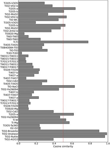
An analysis using all 50 candidates would require a considerable amount of time. Therefore, we performed prescreening using the cosine similarity described in Section 5. Figure 4 shows the cosine similarity between the measured XRD data $\mathcal{D}$ and crystal structure factors $\mathcal{F}$ during prescreening. In this figure, the red line denotes the threshold value, which was set to 0.5. The y-axis denotes cosine similarity. We performed the analysis using crystal structure factors with a cosine similarity greater than 0.5. This prescreening narrowed the list from 50 to 12 candidates. This is expected to result in significant reduction in the computational costs.

Figure 4. Cosine similarity between the measurement XRD data $\mathcal{D}$ and the crystal structure factors $\mathcal{F}$ for prescreening. In this figure, the red line denotes the threshold value set at 0.5.

We analyzed the measured XRD data using the 12 candidates that were narrowed down by prescreening. Figure 5 presents the selection results for each temperature obtained using the REMC method. The x- and y-axes denote the candidate crystal structures and the index of the inverse temperature $\mathit{\tau }$. The proposed method could select the true crystal structures of Anatase, Brookite, and Rutile with 100 [%] probability. The crystal structures and results of sampling all 50 candidates were successfully identified (shown in Figure 3). The computation required approximately 1 h, and pre-screening reduced the computational cost by a factor of three. These results indicate that prescreening can effectively improve the efficiency of the calculations. However, prescreening may exclude true crystal structures from the candidates.

Figure 5. Selection result from 12 candidates for each temperature in the REMC method. The x- and the y-axes denote the candidate crystal structures and the index of the inverse temperature $\mathit{\tau }$. This figure shows a visualization of the indicator probability $\mathit{P}(\mathit{g}|\mathit{Y};\mathit{\beta }={\beta }_{\tau })$ [%]. The large index corresponds to lower temperatures. The color scale denotes the sampling frequency of $g_k=1$ on a log scale. The dark red color indicates the presence of crystal structures in the measured sample.

Figure 6(a) shows the fitting results via the profile function in the measurement XRD data. In Figure 6(a), the black and red lines indicate the measured XRD data and the fitting profile functions, respectively. Figure 6(b) shows the peak components of the three crystal structures of $\mathrm{Ti}{\mathrm{O}}_2$: Anatase, Brookite, and Rutile. The red, green, and blue lines indicate the peaks of Anatase, Brookite, and Rutile, respectively. As shown in this figure, the estimated profile function facilitated a good fit of the XRD data. The mean Poisson cost $\mathit{E}(\hat{\mathrm{\Theta }})$ was 5.026.

Figure 6. Result of profile analysis in the measurement XRD data using our method [(a): Fitting result via profile function in the measurement XRD data. In this figure, the black and the red lines indicate the measurement XRD data and the fitting profile functions, respectively. (b): Peak components in three crystal structures of $\mathrm{Ti}{\mathrm{O}}_2$; Anatase, Brookite, and rutile. The red, green, and blue lines indicate the peaks of Anatase, Brookite, and rutile, respectively].

Figure 7 shows the posterior distribution of the peak area ratio in the triangular diagram when the measurement XRD data were analyzed using the proposed method. In Figure 7, the blue dots indicate the sampling results obtained using the REMC method. The units on the axes are percentages [%]. As evident, the results of the area ratio estimation exhibited extremely high precision.

Figure 7. Posterior distribution of the peak area ratio on the triangular diagram when analyzing the measurement XRD data using the proposed method. The units for the axes are percentages [%].

Figure 8 shows an expanded view of the posterior distribution of the peak used to determine its shape of the posterior distribution. In Figure 8, the red, green, and blue histograms correspond to the posterior distributions of Anatase, Brookite, and Rutile, respectively. As evident, the posterior distribution of Rutile, which has the best crystallinity, exhibited a sharper shape than Anatase and Brookite. The shape of the posterior distribution was similar to that of a quadratic function, where the y-axis represents a logarithmic scale. This implies that the posterior distribution exhibits a Gaussian probability distribution shape. The MAP estimate of the ratio was $\mathrm{Anatase}:\mathrm{Brookite}:\mathrm{Rutile}=35.7:31.8:32.5$ [%]. Because the structural ratio of the preparation is $\mathrm{Anatase}:\mathrm{Brookite}:\mathrm{Rutile}=33.3\dot{3}:33.3\dot{3}:33.3\dot{3}$ [%], the proposed method is considered a reasonable estimation.

Figure 8. Expanded view of the posterior distribution of the peak area ratio when analyzing the measurement XRD data using the proposed method. The units for the axes are percentages [%].

Figure 9 shows the posterior distribution of the profile parameters when analyzing the measurement XRD data using the proposed method. The red, green, and blue histograms represent the posterior distributions of Anatase, Brookite, and Rutile, respectively. Figure 9(a–d) show the peak height $\mathit{h}$, peak shift $\mathit{\mu }$, Gaussian – Lorentz ratio $\mathit{r}$, and asymmetry parameter $\mathit{\alpha }$, respectively. Figure 9(e,f) show the Gaussian width $\mathrm{\Sigma }(x_i;u_k,v_k,w_k,{\alpha }_k)$ and the Lorentz width $\mathrm{\Omega }(x_i;u_k,v_k,w_k,{\alpha }_k)$, where $x_i$ is $2\mathit{\theta }=60$ [°]. As indicated in part (a) of this figure, the height $\mathit{h}$ can be estimated with high precision using the proposed method. The figure shows that the peak shifts for all three crystal structures were positive ($\mathit{\mu }=0.04\sim 0.06$). This may be attributed to minute calibration deviations in the measurement device such as eccentricity and zero-point errors. As shown in parts (e) and (f) of this figure, the peak width of Rutile was narrow, indicating good crystallinity. Furthermore, we confirmed that Rutile with good crystallinity exhibited a sharp posterior distribution shape for most of the profile parameters. By contrast, Brookite with poor crystallinity, tended to exhibit a broad posterior distribution. This indicates that a structure with good crystallinity provides a highly precise estimation.

Figure 9. Posterior distribution of the profile parameters in the measurement XRD data. The red, green, and blue histograms correspond to the posterior distribution of Anatase, Brookite, and rutile, respectively. [(a): Peak height $\mathit{h}$, (b): Peak shift $\mathit{\mu }$, (c): Gauss-Lorentz ratio $\mathit{r}$, and (d): asymmetry parameter $\mathit{\alpha }$]. (e) and (f) are Gauss width $\mathrm{\Sigma }(x_i;u_k,v_k,w_k,{\alpha }_k)$ and Lorentz width $\mathrm{\Omega }(x_i;u_k,v_k,w_k,{\alpha }_k)$, where $x_i$ is $2\mathit{\theta }=60$ [${ }^{\circ }$]. The black dot-dash line is a true parameter of the profile function.

8.2. Analysis in measured data of non-uniform mixing ratios

Here, we show the analysis results for the measured data of non-uniform mixing ratios. We measured the samples with two different mixing ratios: (Case-01) $\mathrm{Rutile}/\mathrm{Anatase}=80/20\mathrm{mass}\mathrm{\%}$ and (Case-02) $\mathrm{Brookite}/\mathrm{Rutile}/\mathrm{Anatase}=97/1/2\mathrm{mass}\mathrm{\%}$. In addition to these ratios, the conditions were identical to those described in Section 8.1. The proposed method was applied to the measured data in both cases. The data for Case-01 and Case-02 are shown in Figures B1 and B5 of Appendix B, respectively.

First, we present the analysis results for Case-01. The data for Case-01 were included in Anatase and Rutile. Prescreening was used to reduce the number of candidates from 50 to 8. Figure 10 presents the selection results for each temperature using the REMC method. The x- and y-axes denote the candidate crystalline phase structures and the index of the inverse temperature $\mathit{\tau }$. The proposed method could select the true crystalline phase structures, which were Anatase and Rutile with a probability of 100 [%]. As shown in Figure 10, Anatase was not sampled using the REMC method at high temperatures. As evident, the determination of Anatase is more challenging than that of Rutile. This indicates that estimating structures with small component ratios is difficult. The fitting results are presented in Figure B1 in Appendix B.

Figure 10. Selection result for each temperature in the REMC method in case-01. The x- and the y-axes denote the candidate crystal structures and the index of the inverse temperature $\mathit{\tau }$. This figure shows a visualization of the indicator probability $\mathit{P}(\mathit{g}|\mathit{Y};\mathit{\beta }={\beta }_{\tau })$ [%]. The large index corresponds to lower temperatures. The color scale denotes the sampling frequency of $g_k=1$ on a log scale. The dark red color indicates the presence of crystalline phase structures in the measured sample.

Second, we present the analysis results for Case-02. The data for Case-02 included Anatase, Brookite, and Rutile. These data have a significantly low ratio of Anatase and Rutile. In particular, Rutile accounted for only 1%. Prescreening was used to reduce the number of candidates from 50 to 15. Figure 11 presents the selection results for each temperature obtained using the REMC method. The x- and y-axes denote the candidate crystalline phase structures and the index of the inverse temperature $\mathit{\tau }$. The proposed method selected Brookite and Anatase as the MAP estimation. The two selected structures were included in the true structures. Surprisingly, we succeeded in detecting Anatase, which accounted for only 2%. As shown in Figure 11, the estimation of Anatase, which has a low mixing ratio, was difficult. However, it can be confirmed that Rutile was not selected by the proposed method. We consider this a reasonable result because Rutile accounted for only 1% of the measured sample. The figure also shows that the $\mathrm{Ti}{\mathrm{O}}_2$ of $\mathrm{Mn}{\mathrm{O}}_2$ structure type was selected with a probability of approximately 50%. Table 2 lists the cell lattice parameters of $\mathrm{Mn}{\mathrm{O}}_2$ and Rutile crystal structures in $\mathrm{Ti}{\mathrm{O}}_2$ [19,21]. The $\mathrm{Ti}{\mathrm{O}}_2$ of $\mathrm{Mn}{\mathrm{O}}_2$ structure type was obtained from literature [19]. As shown in the table, $\mathrm{Mn}{\mathrm{O}}_2$ and Rutile crystalline phase structures are similar. Therefore, it was suggested that $\mathrm{Mn}{\mathrm{O}}_2$ structure type should be sampled instead of Rutile. Notably, the $\mathrm{Ti}{\mathrm{O}}_2$ of $\mathrm{Mn}{\mathrm{O}}_2$ structure type was not selected as the MAP solution. Our method may suggest a crystal structure similar to the true crystal structure by presenting a low probability of existence if the candidate does not contain a true crystalline phase structure. It is important to confirm the behaviour when the true crystalline phase structure is not included and when the crystal lattice is scaled, and this will be addressed in future work. The fitting results are shown in Figure B5 in Appendix B.

Figure 11. Selection result for each temperature in the REMC method in case-02. The x- and the y-axes denote the candidate crystal structures and the index of inverse temperature $\mathit{\tau }$. This figure shows a visualization of the indicator probability $\mathit{P}(\mathit{g}|\mathit{Y};\mathit{\beta }={\beta }_{\tau })$ [%]. The large index corresponds to lower temperatures. The color scale denotes the sampling frequency of $g_k=1$ on a log scale. The dark red color indicates the presence of crystalline phase structures in the measured sample.

Table 2. Cell lattice parameters of $\mathrm{Mn}{\mathrm{O}}_2$ and rutile crystal structure types in $\mathrm{Ti}{\mathrm{O}}_2$ [19,21].

Structure	Chemical	Length [nm]			Angle [degree]
Type	Composition	$\mathit{a}$	$\mathit{b}$	$\mathit{c}$	$<\mathit{\alpha }$	$<\mathit{\beta }$	$<\mathit{\gamma }$
Rutile	$\mathrm{Ti}{\mathrm{O}}_2$	0.30	0.46	0.46	90	90	90
$\mathrm{Mn}{\mathrm{O}}_2$	$\mathrm{Ti}{\mathrm{O}}_2$	0.29	0.49	0.94	90	90	90

9. Conclusion

The knowledge of the probability that a sample contains a candidate crystal structure from full-range XRD data considering both the diffraction angles of the peaks and the profile functions, is essential. This study aimed at the Bayesian estimation of the structure contained in a sample from a large number of crystal structure candidates in the analysis of XRD data. Therefore, indicator vectors were introduced into the profile function and the XRD data were analyzed by sampling the posterior distribution using the REMC method. Consequently, we succeeded in identifying the true crystal structures of 50 candidates with high probability. The proposed method also estimated the mixing ratio of the selected crystal structures with high precision.

In this study, we provide reasonable results that allow clearer identification of the crystal structure for more crystalline structures. Surprisingly, our method successfully detected crystal structures that accounted for only 2 [%] of the sample. However, a crystal structure that contained only 1 [%] of the sample could not be detected, although we proposed a similar crystal structure with low probability, suggesting a reasonable result. Our method is a highly sensitive and probabilistic analysis method that can automatically identify crystal structures from full-range XRD data.

Disclosure statement

No potential conflict of interest was reported by the author(s).

Additional information

Funding

This work was supported by MEXT/JSPS KAKENHI Grant Numbers [18K05191, and 19K12154].

Appendix A.

Fitting results in artificial data

We performed a calculation experiment with the artificial data. It was assumed that the XRD data were measured for a sample containing the three crystal structures of $\mathrm{Ti}{\mathrm{O}}_2$: Anatase, Brookite, and Rutile. We generated artificial data based on a set of true parameters and the model defined in Section 3. Table B1 lists the true parameters of the profile function for the artificial data. We set the x-axis $2\mathit{\theta }$ between 10° and 60° in increments of 0.02[${ }^{\circ }$], such that $2\mathit{\theta }$ is $\mathit{x}=(10.00,10.02,10.04,\dots ,60.00{)}^{\mathrm{T}}$. The background parameters ${\mathrm{\Theta }}_{\mathrm{B}}$ were set to $\mathit{a}=5000.0$, ${\sigma }_{\mathit{bg}}=6.0$, $\mathit{b}=10.0$, $r_{\mathit{bg}}=0.80$. We performed the analysis using the proposed method without knowing the crystal structure of the sample. The purpose of this experiment was to select the true crystal structures (Anatase, Brookite, and Rutile of $\mathrm{Ti}{\mathrm{O}}_2$) from the XRD data.

Figure B2 shows the selection results obtained using the proposed method on artificial XRD data. This figure shows the indicator probability $\mathit{P}(\mathit{g}=1|\mathit{Y})$ [%]. The proposed method estimates the crystal structure of a sample from 50 candidates. Candidate crystal structures were obtained from AtomWork as described in Section 7.4. The y- and x-axes indicate the crystal structure and indicator probability, respectively. As evident, the proposed method could select true crystal structures, that is, Anatase, Brookite, and Rutile, from 50 candidates with 100 [%] probability.

Figure B3(a) shows the fitting results obtained using the profile function for the artificial data. In Figure B3(a), the black and red lines represent the artificial data and fitting profile function, respectively. Figure B3(b) shows the peak components of the three crystal structures of $\mathrm{Ti}{\mathrm{O}}_2$: Anatase, Brookite, and Rutile. The red, green, and blue lines represent peaks of Anatase, Brookite, and Rutile, respectively. As evident, the estimated profile function provides a good fit. The mean Poisson cost $\mathit{E}(\hat{\mathrm{\Theta }})$ was 4.476, which is close to the true cost of 4.469 given by the true parameters.

Figure B4 shows the posterior distributions of the profile parameters. The red, green, and blue histograms represent the posterior distributions of Anatase, Brookite, and Rutile, respectively. Figure B4(a–d) show the peak height $\mathit{h}$, peak shift $\mathit{\mu }$, Gaussian–Lorentz ratio $\mathit{r}$, and asymmetry parameter $\mathit{\alpha }$, respectively. Figure B4(e,f) show the Gaussian widths $\mathrm{\Sigma }(x_i;u_k,v_k,w_k,{\alpha }_k)$ and Lorentz width $\mathrm{\Omega }(x_i;u_k,v_k,w_k,{\alpha }_k)$, where $x_i$ is $2\mathit{\theta }=60$ [${ }^{\circ }$]. In Figure B4, the black dot-dashed line represents the true parameter of the profile function. As evident, the expectation of the posterior distribution is in good agreement with the true values. In addition, the shape of the histogram is a quadratic function, where the y-axis represents the log scale. This implies that the posterior distribution exhibits a Gaussian probability distribution shape. Therefore, this experiment confirms that the proposed method works well on artificial data.

Appendix B.

Data and Fitting in Section 8.2

Figure B1 and Figure B5 show the fitting result of Case-01 and Case-02 in Section 8.2, respectively. In Figure (a), the black and red lines represent the measurement XRD data and the fitting profile function, respectively. Figure (b) shows the peak components. The red, green, and blue lines represent peaks of Anatase, Brookite, and Rutile, respectively.

Figure B1. Result of profile analysis in case-01 using our method [(a): Fitting result via profile function in the measurement XRD data. The black and the red lines represent the measurement XRD data and the fitting profile function, respectively. (b): Peak components in two crystal structures of $\mathrm{Ti}{\mathrm{O}}_2$; Anatase and rutile. The red and blue lines denote peaks of Anatase and rutile, respectively].

Table B1. True parameter of profile function in artificial data. We assumed that the XRD data were measured on a sample containing three crystalline phase structures of $\mathrm{Ti}{\mathrm{O}}_2$: Anatase, Brookite, and rutile.

${\mathrm{\Theta }}_{\mathrm{S}}$	Rutile	Brookite	Anatase
$h_k$	5000.0	5000.0	5000.0
${\mu }_k$	0.05	0.05	0.05
${\alpha }_k$	0.80	0.80	0.80.
$r_k$	0.50	0.50	0.50
$u_k$	0.005	0.005	0.005
$v_k$	0.005	0.005	0.005
$w_k$	0.05	0.10	0.15
$s_k$	0.10	0.15	0.20
$t_k$	0.005	0.005	0.005

Figure B2. Selection result from 50 candidates for each temperature using the REMC method for artificial XRD data. The x- and the y-axes denote the candidate crystal structures and the index of the inverse temperature $\mathit{\tau }$. This figure shows a visualization of the indicator probability $\mathit{P}(\mathit{g}|\mathit{Y};\mathit{\beta }={\beta }_{\tau })$ [%]. The large index corresponds to lower temperatures. The color scale denotes the sampling frequency of $g_k=1$ on a log scale. The dark red indicates the presence of the crystal structure in the measured sample.

Figure B3. Result of profile analysis in the artificial data using our method [(a): Fitting result via profile function in the artificial data. In this figure, the black and the red lines indicate the artificial data and the fitting profile function, respectively. (b): Peak components in three crystal structures of $\mathrm{Ti}{\mathrm{O}}_2$: Anatase, Brookite, and rutile. The red, green, and blue lines indicate peaks of Anatase, Brookite, and rutile, respectively].

Figure B4. Posterior distribution of the profile parameters in the artificial data. The red, green, and blue histograms are the posterior distribution of Anatase, Brookite, and rutile, respectively. [(a): Peak height $\mathit{h}$, (b): peak shift $\mathit{\mu }$, (c): Gauss-Lorentz ratio $\mathit{r}$, and (d): asymmetry parameter $\mathit{\alpha }$]. (e) and (f) are Gauss width $\mathrm{\Sigma }(x_i;u_k,v_k,w_k,{\alpha }_k)$ and Lorentz width $\mathrm{\Omega }(x_i;u_k,v_k,w_k,{\alpha }_k)$, where $x_i$ is $2\mathit{\theta }=60$ [degree]. The black dot-dashed line denotes the true parameter of the profile function.

Figure B5. Result of profile analysis in case-02 using our method [(a): Fitting result via profile function in the measurement XRD data. The black and red lines denote the measurement XRD data and the fitting profile function, respectively. (b): Peak components in two crystal structures of $\mathrm{Ti}{\mathrm{O}}_2$; Anatase and Brookite. The red and green lines denote peaks of Anatase and Brookite, respectively].

References

- Press WH, Teukolsky SA. Savitzky-golay smoothing filters. Comput Phys. 1990;4(6):669–20. doi:10.1063/1.4822961
- Taupin D. Automatic peak determination in x-ray powder patterns. J Appl Crystallogr. 1973;6(4):266–273. doi:10.1107/S0021889873008666
- Huang TC. Precision peak determination in x-ray powder diffraction. Aust J Phys. 1988;41(2):201–212. doi:10.1071/PH880201
- Surdu V-A, Győrgy R. X-ray diffraction data analysis by machine learning methods—a review. Appl Sci. 2023;13(17):9992. doi: 10.3390/app13179992
- Greasley J, Hosein P. Exploring supervised machine learning for multi-phase identification and quantification from powder X-ray diffraction spectra. J Mater Sci. 2023;58:1–15. doi:10.1007/s10853-023-08343-4
- Fancher CM, Han Z, Levin I, et al. Use of Bayesian inference in crystallographic structure refinement via full diffraction profile analysis. Sci Rep. 2016;6:8. doi: 10.1038/srep31625
- Mikhalychev A, Ulyanenkov A. Bayesian approach to powder phase identification. J Appl Crystallogr. 2017 Jun;50(3):776–786. doi: 10.1107/S1600576717004393
- Suzuki Y. Automated data analysis for powder X-ray diffraction using machine learning. Synchrotron Radiat News. 2022;35(4):9–15. doi:10.1080/08940886.2022.2112496
- Momma K, Izumi F. VESTA: a three-dimensional visualization system for electronic and structural analysis. J Appl Crystallogr. 2008 Jun;41(3):653–658. doi: 10.1107/S0021889808012016
- Toraya H. Array-type universal profile function for powder pattern fitting. J Appl Crystallogr. 1990 Dec;23(6):485–491. doi: 10.1107/S002188989000704X
- Wertheim GK, Butler MA, West KW, et al. Determination of the gaussian and lorentzian content of experimental line shapes. Rev Sci Instrum. 1974;45(11):1369–1371. doi: 10.1063/1.1686503
- Hukushima K, Nemoto K. Exchange Monte Carlo method and application to spin glass simulations. J Phys Soc Jpn. 1996;65(6):1604–1608. doi:10.1143/JPSJ.65.1604
- Nagata K, Sugita S, Okada M. Bayesian spectral deconvolution with the exchange Monte Carlo method. Neural Netw. 2012;28:82–89. doi:10.1016/j.neunet.2011.12.001
- Rietveld HM, HM Rietveld. Line profiles of neutron powder-diffraction peaks for structure refinement. Acta Crystallogr. 1967;22(1):151–152. doi:10.1107/S0365110X67000234
- Rietveld HM. A profile refinement method for nuclear and magnetic structures. J Appl Crystallogr. 1969 Jun;2(2):65–71. doi: 10.1107/S0021889869006558
- Rodríguez-Carvajal J. Recent advances in magnetic structure determination by neutron powder diffraction. Phys B Condens Matter. 1993;192(1–2):55–69. doi:10.1016/0921-4526(93)90108-I
- Akselrud L, Grin Y. Wincsd: software package for crystallographic calculations (version 4). J Appl Crystallogr. 2014;47(2):803–805. doi:10.1107/S1600576714001058
- Xu Y, Yamazaki M, Villars P. Inorganic materials database for exploring the nature of material. Jpn J Appl Phys. 2011 Nov;50(11S):11RH02. doi: 10.1143/JJAP.50.11RH02
- Akimoto J, Gotoh Y, Oosawa Y, et al. Topotactic oxidation of ramsdellite-type li0.5tio2, a new polymorph of titanium dioxide: Tio2(r). J Solid State Chem. 1994;113(1):27–36. doi: 10.1006/jssc.1994.1337
- Latroche M, Brohan L, Marchand R, et al. New hollandite oxides: Tio2(h) and k0.06tio2. J Solid State Chem. 1989;81(1):78–82. doi: 10.1016/0022-4596(89)90204-1
- Kim D-W, Enomoto N, Nakagawa Z-E, et al. Molecular dynamic simulation in titanium dioxide polymorphs: rutile, brookite, and anatase. J Am Ceram Soc. 1996;79(4):1095–1099. doi: 10.1111/j.1151-2916.1996.tb08553.x