
 ?Mathematical formulae have been encoded as MathML and are displayed in this HTML version using MathJax in order to improve their display. Uncheck the box to turn MathJax off. This feature requires Javascript. Click on a formula to zoom.
ABSTRACT
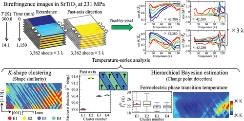
A new machine learning approach that transforms time-series analysis into temperature-series analysis is introduced to analyze stress-induced ferroelectricity in SrTiO3 at 231 MPa using birefringence images observed at successive temperatures. The spatial distribution of the temperature-series data for each of the 42,280 pixels was clustered using the multivariate -shape clustering method based on the shape similarity of the temperature dependence. In addition, to obtain the structural and ferroelectric phase transition temperatures,
and
, hierarchical Bayesian temperature-series estimation was performed at each pixel (as a lower level) constrained over the entire cluster (as a higher level) considering the measurement error. Consequently, the K-shape clustering method revealed four clusters corresponding to elongated ferroelectric domains, explained by slight differences in retardance and fast-axis direction. Statistical analysis of the Bayesian posterior probability distribution showed a uniform distribution of
over the sample, but an inhomogeneous distribution of
. The higher
regions exhibited a concentration of stress and/or strain. The Pearson correlation coefficient calculations suggested a strong to moderate relationship between the distribution of TF and the ferroelectric state, while the correlation between Tc and the ferroelectric state was weak or nonexistent. The combination of machine learning and statistics provides a more reliable and less arbitrary approach to analyzing temperature-series data. These multilevel analyses are particularly useful in studying critical phenomena near phase transition temperatures in condensed matter physics.
GRAPHICAL ABSTRACT
IMPACT STATEMENT
Temperature-series analysis, combined with statistics, provides deeper insights into numerous imaging data observed at successive temperatures. This method will bring innovation to study of critical phenomena in condensed matter physics.
1. Introduction
In condensed matter physics, one of the most important research topics is investigation of the complex relationship between temperature () and physical properties, particularly critical phenomena occurring near phase transition temperatures [Citation1]. These phenomena gain an additional layer of complexity when intertwined with changes in external parameters, such as magnetic field, electric field, and pressure. An increase in the number of external parameters generates complex, multivariate data structures that escalate in volume and complexity [Citation2–4]. Traditional analysis methods, which are typically limited to examining variables in isolation, struggle to unravel these complex interactions. To bridge this gap, we have proposed an innovative machine learning approach for analyzing
-dependent data, which is optimized for the study of critical phenomena in condensed matter physics.
Since the 2000s, remarkable progress has been made in imaging techniques for the detection of spatial information regarding physical properties [Citation5–10]. These developments are essential for the study of functional materials and focus on the formation and dynamics of macroscopic structures, such as domains or domain walls that affect magnetic, electrical, and transport properties. Therefore, advanced imaging techniques have become a fundamental part of materials research; however, such techniques have triggered an era of data explosion [Citation6–8]. For example, spectral imaging collects the wavelength () or energy dependence at each pixel to obtain a single image [Citation2,Citation4,Citation5]. Extracting meaningful insights from a large dataset remains challenging despite advances in measurement techniques. Traditional analysis methods, based on averaging data from selective regions of interest, are limited in scope and prone to arbitrary bias. They often fail to analyze the overall trends of complex distributions and may miss local but important details. This generates an opportunity for machine learning, i.e. by applying advanced algorithms, we can extract deeper insights from a large dataset that previously remained inaccessible [Citation11]. Pioneering research in condensed matter physics has involved the use of multivariate analysis methods based on statistics, i.e. principal component analysis [Citation12,Citation13], a multivariate curve resolution technique [Citation14], and nonnegative matrix factorization [Citation15], to analyze spectral imaging data. Although these methods are adept at extracting features by reducing multivariate data to a lower dimension, they prove insufficient at learning from data to make predictions or decisions for new data. Our machine learning approach is designed to analyze
-dependent imaging data, thus providing more accurate and flexible analysis than before.
We developed a novel machine learning approach for analyzing -dependent birefringence imaging data, focusing on stress-induced ferroelectricity in SrTiO
[Citation16–18]. Although such phase transition phenomena have been known for a long time [Citation19–22], the high electrical conductivity caused by strain-induced ferroelectricity at the interface between SrTiO
and LaAlO
has attracted renewed attention [Citation23–26]. Birefringence is a technique that uses the polarization properties of light to reveal both the internal structure and dielectric properties of materials. In this study, to effectively manage and interpret numerous birefringence images at different temperatures, we employ machine learning techniques that focus on unsupervised learning methods such as clustering algorithms [Citation27]. These techniques are important for identifying underlying patterns and correlations not readily apparent in a large dataset. Pioneering research has been conducted on the application of machine learning to the analysis of reflection high-energy electron diffraction images [Citation28–31]. Our previous study reported the application of a
-means clustering technique to the analysis of a birefringence image [Citation18]. However, the analysis of
dependence over numerous images remains a substantial challenge. In this study, we focus on the similarity between time-series and
-series data for efficient analysis of successive images.
Because -series analysis methods have not yet been developed, our approach attempts to simply convert the time variables into the
variables. Time-series analysis is a major topic in machine learning with enormous related knowledge available [Citation32,Citation33]; therefore, the application of these methods to
-series analysis can lead to considerable development in condensed matter physics. First, we recognize that series data have the following unique properties: (1) a distinct sequential order, which is essential for accurate interpretation; (2) a relational dynamic, where each data point depends on its neighbors; (3) a contextual essence, where the true value of the series is unlocked when viewed as a cohesive whole. With these insights, the
-dependent birefringence images of the stress-induced ferroelectricity in SrTiO
are analyzed. For spatial distribution analysis, we use the
-shape clustering method to identify the ferroelectric domain structures [Citation34]. In traditional time-series analysis, Euclidean distance and dynamic time warping are commonly used although they are sensitive to variations in the data scale and can overlook similarities in shapes [Citation32,Citation33]. The
-shape clustering method is a specialized technique for clustering based on the shape of time-series data. Shape similarity is one of the most important features that forms the scaling law in condensed matter physics [Citation1]. Furthermore, for the pixel-by-pixel
-series analysis, we use Bayesian
-series estimation to identify the structural and ferroelectric phase transition temperatures (
and
) [Citation35,Citation36]. The Bayesian approach has an important advantage of directly incorporating prior knowledge and uncertainties such as measurement error directly into the modeling process, allowing us to perform comprehensive and probabilistic parameter inference based on the posterior probability distribution. Our combined machine learning approach toward spatial distributions and
variations provides a deeper understanding of complex data structures in earlier impossible ways. This approach overcomes the limitations of traditional analysis methods in condensed matter physics and opens new avenues for exploring various critical phenomena, potentially revolutionizing the way researchers approach a large dataset.
2. Dataset for analysis
2.1. Birefringence images in SrTiO3
Machine learning was applied to -series birefringence imaging data for the stress-induced ferroelectricity of SrTiO
. Under stress-free conditions, SrTiO
undergoes a structural phase transition at
K from the cubic paraelectric state to the tetragonal quantum paraelectric state, where the ferroelectric state is suppressed by quantum fluctuations [Citation37–39]. The quantum paraelectric state undergoes ferroelectric phase transition upon the application of stress or strain [Citation19–22,Citation24–26,Citation40–42]. For a SrTiO
thin film, strain-induced ferroelectricity appears at room temperature because of the lattice mismatch between the substrate and the thin film [Citation24–26,Citation40–42]. Similarly, for a SrTiO
bulk sample, when the external force (
) is applied along
, whose direction corresponds to the cubic phase,
increases from 105 K with increasing
[Citation20–22]. At
K, ferroelectric phase transition occurs, resulting in spontaneous polarization along
; moreover,
increases with increasing
[Citation20–22]. In the previous experimental studies of the stress-induced ferroelectricity in SrTiO
, the value of
has been considered as stress because the external and internal forces (
stress) are balanced. Unlike hydrostatic pressure experiments wherein
is applied uniformly in all directions, the stress caused by
is unevenly distributed throughout the sample. This is because
is applied from only one axial direction, and stress tends to be distributed perpendicularly to
. Therefore, the stress-induced ferroelectric state may also be inhomogeneous because of the stress distribution. According to a study conducted by Müller et al. in Ref [Citation19], when
, the relationship between the converted stress (
) and
is given by
Reportedly, this relationship also holds when [Citation16]. In this study, we used imaging techniques to evaluate the local stress and ferroelectric domain structure from the distributions of
and
on a pixel-by-pixel basis.
We obtained -dependent birefringence images of the SrTiO
substrate at
MPa applied along
when
decreases from 300.0 to 14.1 K, as already reported in Ref [Citation16]. To fully understand the stress-induced ferroelectric phase transition, our analysis focuses on capturing the inhomogeneous distribution of critical phenomena in the substrate. Because the SrTiO
substrate at
MPa belongs to the plastic region, the linear relationship between stress and strain disappears [Citation17]. According to theoretical studies on SrTiO
thin films [Citation43–47], the lattice distortion functions as a driving force for ferroelectricity and
is expected to increase with increasing strain. However, because our experimental method cannot help determine whether the observed birefringence is more influenced by stress or strain, we do not distinguish between stress and strain.
The measurement principles required for machine learning with respect to analyzing the -series birefringence imaging data are described as follows. Incident white light with circular polarization expressed as the Stokes parameters (
) is passed through the SrTiO
(110) substrate along
, and the polarization state of the transmitted light is obtained as (
) [Citation48,Citation49]. The polarization state at each point of
pixels can be obtained through a single measurement using a CCD camera with polarizing plates. When the refractive indices along the orthogonal principal optical axes are defined as
and
for the slow and fast axes with
, respectively, the birefringence (
) and retardance (
) are expressed as follows:
where represents the sample thickness (
mm), and the fast-axis direction (
) corresponds to the direction for
. To elucidate the large value of
exceeding
, we observed the transmitted light separated into three different
s at 523, 543, and 575 nm using bandpass filters [Citation50]. In case of the SrTiO
substrate at
MPa, the value of
helps evaluate the amount of spontaneous polarization due to the Pockels effect [Citation51,Citation52] and stress and/or strain due to the photoelastic effect [Citation16,Citation17]. In addition, the
direction reflects the crystal orientation; therefore, its distribution image can be used to infer the distribution of the spontaneous polarization direction [Citation53–56]. As reported in Ref [Citation16], show images of
and
at 130.9 K, corresponding to the cubic paraelectric state. Notably, these images are converted at
nm. Stripe patterns due to the slip planes appear even at 300.0 K, and their directions coincide with the directions of the projection of
onto
. shows an image of the
stripe pattern; the origin of this image can be attributed to the fact that the fast-axis directions indicated by the arrows differ by a few degrees between the elongated domains. These images show considerably similar distributions to those observed at 30.0 (paraelectric tetragonal state) and 14.1 K (ferroelectric state) shown in of Ref [Citation18]. Because the
and
values correspond to a certain cross-section of the Poincaré sphere comprising the Stokes parameters [Citation18,Citation48,Citation49], the analysis results from different approaches may appear different. Furthermore, it is challenging to quantitatively assess the amount and direction of spontaneous polarization by simultaneously examining the
and
distribution images. Therefore, a multivariate analysis using machine learning must be developed to mine the hidden information in
-series birefringence imaging data.
Figure 1. In SrTiO(110) substrate at an external force of
MPa applied along
, images at 130.9 K of (a) retardance
and (b) fast-axis direction
. The large open arrows schematically indicate
. In (a), the cross marks indicate the analysis position, as shown in . The order is defined from the left end to the right end as a1 to a7. (c) Schematic illustration of the origin of the stripe pattern along
. The arrows are the fast-axis directions and differ by a few degrees between the elongated domains.
![Figure 1. In SrTiO 3(110) substrate at an external force of σ=231 MPa applied along [001]c, images at 130.9 K of (a) retardance δ and (b) fast-axis direction ψ. The large open arrows schematically indicate σ. In (a), the cross marks indicate the analysis position, as shown in Figure 4. The order is defined from the left end to the right end as a1 to a7. (c) Schematic illustration of the origin of the stripe pattern along ⟨111⟩c. The arrows are the fast-axis directions and differ by a few degrees between the elongated domains.](/cms/asset/96ba04cc-140f-4d5c-b607-39ac4bfa4749/tstm_a_2342234_f0001_oc.jpg)
In our previous research, reported in Ref [Citation18], we applied the -means clustering method to the birefringence imaging data to observe the ferroelectric domains in SrTiO
at 231 MPa. This approach involved subtraction between the 30.0-K and 14.1-K datasets on a pixel-by-pixel basis, and it effectively simplified the
-series data for spatial clustering. Our results identified three distinct clusters (D1–D3, see Supplementary materials), each with unique characteristics. Cluster D1 exhibited large spontaneous polarization and disordered crystal orientation, indicating stress and/or strain concentration. Conversely, cluster D3 showed small spontaneous polarization but a more uniform distribution and less disordered crystal orientation. Furthermore, cluster D2 showed intermediate properties. This difference between clusters highlights the complex state of the stress-induced ferroelectricity in SrTiO
. However, our method could not adequately visualize the domain structures along
; this limitation is attributed to the reduction of
-series information in the clustering process. Therefore, there is an urgent need for advanced analysis techniques that comprehensively integrate spatial information and
-dependent data. The development of such methods could considerably improve the accuracy of visualization of ferroelectric domain structures and provide deeper insights into the complex
dependence of birefringence in case of SrTiO
. This approach will provide a new perspective for the analysis of critical phenomena in condensed matter physics.
2.2. Preprocessing of birefringence imaging data
We preprocessed our data sets to efficiently perform machine learning without sacrificing accuracy. Focusing on the SrTiO substrate, birefringence imaging data at each
were extracted at 42,280 pixels (302
140 pixels). As previously described in Ref [Citation18], the Stokes parameters (
) and (
) at each
were averaged over a 3
3 pixel area using the moving average method. Because the sample position shifts with decreasing
, the analysis locations must be adjusted by one pixel unit and averaging is most effective in suppressing the effect of deviations of less than one pixel. Using these averaged Stokes parameters, we subsequently defined the important variables
and
, setting the stage for our subsequent analysis on the Poincaré sphere [Citation18]. The angle
, corresponding to
, was defined within the range
with a periodicity of
. The axial direction
, reflecting the direction of the fast or slow axis, was restricted to
, also with a periodicity of
. With these definitions, we generally expressed the retardance as
, where
, and the fast-axis direction as
. Whenever
exceeds
, the angle
folds back at 0
or 180
; therefore, the variables for
and
change concurrently. The accuracy of machine learning predictions can be improved using the
-series data for the three
s without corrections for these variables on a pixel-by-pixel basis [Citation18].
Because the variables and
are angular measures, we adopted circular statistics for our analysis [Citation57,Citation58]. This approach allows us to consider angles as vectors, which simplifies their computation and interpretation. From Ref [Citation18], the mean (or maximum likelihood estimate) of
and
is expressed as follows:
where denotes the number of data points and
represents the mean resultant length. The value of
varies between 0 and 1 and indicates the alignment of the distribution, i.e. values closer to 1 signify a well-aligned distribution. The maximum likelihood estimation of
and
can be reformulated as follows:
This allows angles to be treated as linear statistics [Citation57,Citation58]. Consequently, the four variables (,
,
, and
) are derived from
and
at the
-th measurement point. After successfully applying circular statistics, we extended this procedure to our datasets for three different
s, creating a 42,280
12 matrix for a birefringence image. In this study, it is necessary to further develop a method for analyzing the numerous images observed at successive temperatures. Because all
-series data are standardized for each variable before machine learning, as discussed later,
and
are not necessary for analyzing the
dependence only at a pixel. However, the
-shape clustering would be more reliable by preserving information regarding the distribution within the substrate. Therefore, as a preprocessing of the 12-variable
-series data for 42,280 pixels, we calculated
and
for each birefringence image. These careful preprocessing steps help accurately analyze our
-series birefringence imaging data and set the stage for insightful machine learning.
The stress apparatus made of Cu thermally shrinks with decreasing , causing a shift in the sample position [Citation59]. With 300.0 K as reference, the birefringence image at 14.1 K showed shifts of 23 pixels to the left and 4 pixels to the bottom. Therefore, we manually corrected the sample position by one pixel unit in all images. Previously, we selected as homogeneous a region of the sample as possible and averaged the data within a 10–30
10–30-pixel area to ensure that the shift of less than one pixel was negligible [Citation16]. However, since the
-series data is analyzed on a pixel-by-pixel basis, the 3
3 pixel averaging preprocessing proved insufficient in regions where the amount of birefringence changes abruptly. In these regions, because small jumps appear in
and
curves, conventional time-series analysis methods, which mainly focus on the temporal differences of the changes, would cause serious problems [Citation32,Citation33]. In this study, we adopted the multivariate
-shape clustering method [Citation34] because it is robust to changes in data scale and time deviations, effectively classifying data into the same cluster based on shape similarity. It also maximizes the cross-correlation within a cluster, increasing the likelihood of grouping similar data. Furthermore, for the
-series analysis using the
and
curves, such jumps will inevitably have a negative impact on the estimation of
and
values. Because it is impossible to check the
-series data for all 42,280 pixels, the Bayesian
-series estimation should be used, considering error factors based on certain criteria [Citation35,Citation36]. Using the Bayesian posterior probability distribution, the confidence and accuracy of the estimates can be quantitatively understood, allowing discussion of the relationship between the stress and/or strain concentration and the ferroelectric state.
3. Data analysis procedure
Our computer was equipped with an Intel(R) Core(TM) i9-13900K CPU running up to 5.80 GHz and implemented 128 GB of memory. To meet the demands of datasets larger than 20 GB, we avoided data input/output bottlenecks on hard disk drives and increased data throughput many times by installing a solid-state drive. For the -shape clustering analysis, we used the tslearn package (version 0.5.3.2), a common tool for time-series analysis in the Python environment (version 3.11.1). To determine the optimal number of clusters
, a combination of methods was used, including the elbow method, silhouette method, and gap statistic [Citation60], all of which are integrated in the tslearn package. The computation time, inherently dependent on
, was approximately half a day for computing nine different cluster types ranging from
to 10. For Bayesian
-series estimation, we used the computational power of the Hamiltonian Monte Carlo (HMC) algorithm, a sophisticated technique for Markov chain Monte Carlo (MCMC) simulations, run through the rstan package (version 2.26.23) in the R environment (version 4.1.2). To efficiently process the Bayesian
-series estimation for each of the 42,280 pixels, we employed a strategy that used the parallel package (version 4.1.2), foreach package (version 1.5.2), and doParallel package (version 1.0.17) for parallel computations. This methodology helped us take advantage of parallel processing on up to 32 cores. The computational time depended not only on the number of iterations and chains in the MCMC simulations, but also on the settings of the prior distribution. After extensive optimization, we could estimate the fast-axis directions in a few minutes, as well as
and
in approximately a day and a week, respectively. By applying
-series analysis using hierarchical Bayesian
-series estimation, we aim to complement our spatial data analysis using
-shape clustering and provide a more holistic understanding of stress-induced ferroelectricity.
Our approach to -series analysis, which relates changes in sample
to changes in time, presents unique challenges and opportunities for deeper insight. To address these challenges, we focus on statistical significance in time-series analysis. In time-series analysis, direct tests of statistical significance often require complex procedures tailored to the unique characteristics of the data. Nevertheless, in our approach, we demonstrate the utility of the exploratory values obtained from the MCMC simulations within the Bayesian framework. These values provide an indirect but an effective approach to assess differences between groups by providing insights into posterior distributions. Because of the large sample size in the MCMC simulations, the
test and the Wilcoxon rank sum test are prone to type 1 errors, but Cohen’s
remains robust to them [Citation61,Citation62]. Cohen’s
with Hedges’ correction was calculated using the effsize package (version 0.8.1) in the R environment. Cohen classified effect sizes as small (
), medium (
), and large (
). According to Cohen’s guidelines,
indicates a subtle but noticeable difference,
indicates a moderate and observable difference, and
indicates a substantial and practically significant difference between two groups [Citation61,Citation63]. Statistical treatment using Cohen’s
with Hedges’ correction is important for drawing robust conclusions from
-dependent patterns. The normal-based 95% confidence interval calculated using the normal distribution method is based on the standard error and the assumption that our estimates follow a normal distribution. However, because the data may not follow a parametric distribution, we used the bootstrap 95% confidence interval, which is derived by bootstrap resampling and does not assume a specific distribution. This analysis was performed in the R environment using the boot package (version 1.3.28).
4. Results and discussion
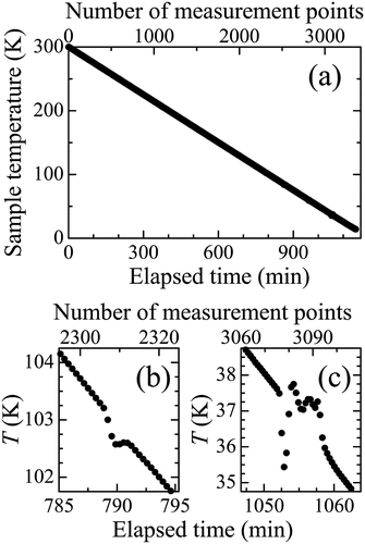
shows the time and measuring point evolution of sample . As described in Ref [Citation16], our measurements continuously recorded 3,362 sheets
3
s of the birefringence imaging data from 300.0 to 14.1 K while carefully controlling the decrease of
at a fixed rate of
K/min. Because of the consistent relationship between
and time, which accurately reflects the order and interval characteristics of the series data, it is feasible to apply the
-series birefringence imaging data to machine learning using
-shape clustering and hierarchical Bayesian
-series estimation.
Figure 2. (a) Sample temperature variation with time and measurement points. Regions of insufficient temperature control, (b) affecting the determination of the structural phase transition temperature, and (c) affecting the determination of ferroelectric phase transition temperature.
4.1. K-shape clustering
To comprehensively characterize the spatial information, the -series birefringence imaging data were analyzed using the
-shape clustering method. shows the
dependence of
and
calculated at each
. The
curves indicate that the distribution of
becomes large below 30 K because ferroelectric phase transition occurs and spontaneous polarization is inhomogeneously distributed over the substrate, as reported in Ref [Citation18]. The
curves for different
s show a remarkable difference near
and
. Furthermore, the
curves also seem to slightly differ in the same
regions. This is attributed to the
folding back at 180
when
exceeds
at 523 and 543 nm. shows the
dependence of the 4-variable
3-
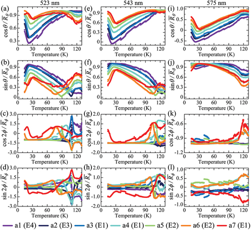
for each pixel, specifically, the seven pixels shown in , selected from a total of 42,280 pixels. These curves show numerous small jumps due to the continuous shift of the sample position. Based on a comparison of with , owing to the considerably small variation in
and
below 30 K, the shape of the
-dependent curves of 12 variables divided by their coefficients remains almost unchanged. Furthermore, around
,
changes considerably because of the folding back of
. These coefficients tend to effectively expand the difference between the pixels in the
-series data. The
and
estimates are expected to further improve the accuracy of the
-shape clustering process. However, as shown in ), it is difficult to completely control sample
owing to the limitations of experimental techniques, resulting in small fluctuations within certain
ranges. Such fluctuations temporarily impose a nonintrinsic external force on the substrate, resulting in small birefringence anomalies that can be observed across all pixels. This is a considerable difference between the
-series data and the time-series data. In conventional time-series analysis, the order can easily affect the results; therefore, the
-shape clustering method, which focuses on shape similarity, is preferred in condensed matter physics [Citation32–34]. Although there is no intrinsic thermal hysteresis in SrTiO
, we entered machine learning in its measured order in this study.
Figure 3. Temperature dependence of the mean resultant length (a) and (b)
for
, 543, and 575 nm.
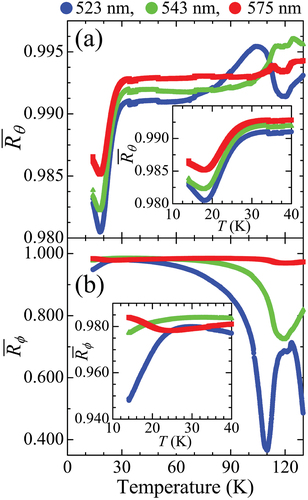
Figure 4. Four variables (,
,
, and
) as a function of temperature at (a–d)
nm, (e–h) 543 nm, and (i–l) 575 nm. Analysis positions a1 to a7 and the corresponding cluster numbers to which they belong.
To optimize computational efficiency, we preprocessed the 42,280-pixel 12-variable
-series data between 130.9 and 14.1 K by averaging every four
points, resulting in each
-series containing 346 points with an approximate step of 0.34 K. For the multivariate
-shape clustering method, determining the number of clusters
in advance is imperative. shows the results of identifying the optimal values of
using the elbow method, silhouette method, and gap statistic [Citation60]. Typically, these methods rarely yield consistent results because each emphasizes different aspects of cluster cohesion and separation. In other words, the elbow method focuses on the variance of the data in the clusters, the silhouette method focuses on the high cohesion in the clusters and the large separation between the clusters, and the gap statistic technique focuses on the difference between the random and real datasets. In this study, because the elbow and silhouette methods indicate
, as shown in , we selected this value. Although these indicators shown in serve as guidelines [Citation60], re-evaluating the validity of
after clustering is essential. shows the division of the 12-variable
-series data into four groups (E1–E4), revealing the elongated clusters along
corresponding to the dislocation. Comparing the multivariate
-shape clustering shown in with the multivariate
-means clustering (D1-D3, see Supplementary materials) [Citation18], we found that clusters E1 and E2 coincide with clusters D1 and D2, indicating large spontaneous polarization in these regions due to stress and/or strain concentration. Conversely, clusters E3 and E4, which correspond to cluster D3, could be regions of low spontaneous polarization and less disordered crystal orientation. shows the number of pixels for each cluster obtained from the
-means and
-shape clustering analyses. This result also corroborates that E1 and E2 correspond to D1 and D2, respectively, E3 and E4 correspond to D3.
Figure 5. Evaluation results for the optimal value of using the (a) elbow method, (b) silhouette method, and (c) gap statistic.
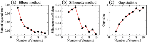
Figure 6. Result of the K-shape clustering obtained from 12 variables of temperature-series data between 130.9 and 14.1 K.
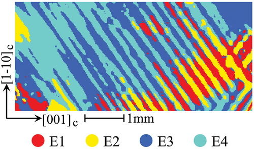
Table 1. Number of pixels in respective clusters determined by K-means and K-shape clustering methods. The K-means clustering data are referenced in Ref. [Citation18].
4.2. Analysis for each cluster
In , it appears that domains E1 and E3 along form one group, while domains E2 and E4 form another. The
dependence of
and
was summed of each cluster to confirm the characteristics for each cluster. The averaged values of the retardance,
, and the fast-axis direction,
, for each cluster were obtained by averaging the difference between the incident and transmitted light of the Stokes parameters at each
, defined as
, as follows:
where represents the difference between the Stokes parameters at the
-th pixel. shows the
dependence of
and
at 575 nm when
and
are rewritten as follows:
Figure 7. Temperature dependence of the (a) averaged retardance, , and (b) averaged fast-axis direction,
, for
nm. In (a), the
curves for E1 and E2 overlap, and the curves for E3 and E4 overlap.
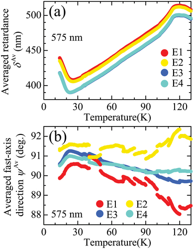
These curves are almost identical to those for 523 and 543 nm, except for the and
regions. In these regions, it is difficult to correctly estimate the value of
from
because we cannot separate the two components of
that fold back at 180
and do not fold back on a pixel-by-pixel basis. In this study, we focused our analysis on
-series data at 575 nm.
In , the curves exhibit a similar shape regardless of the clusters, with two inflection points appearing at
and
. In addition, the values of
are overall higher for E1 and E2 than for E3 and E4 because of stress and/or strain concentration. However, for E1 and E2, the direction of spontaneous polarization may be disturbed because the crystal orientations are disturbed, as discussed in Ref [Citation18]. The slopes of the
curves at
(the ferroelectric state) appear to be steeper for E3 and E4 than for E1 and E2 because the increase in
due to the Pockels effect may be proportional to the superposition of spontaneous polarizations resulting from disturbed crystal orientations. In , the
curves show numerous small jumps due to shifts in the sample position. In particular, the jumps of the
curves for E1 and E2 exhibit opposite trends with almost identical magnitudes in the same
range. As shown in , the effect of less than one pixel misalignment is pronounced because the vertically elongated domains for E1 and E2 alternate along the horizontal direction where the displacement is large. From a crystallographic viewpoint, it is unlikely that the optical principal axis rotates by a few degrees in the cubic or tetragonal phase with decreasing
. However, if the crystal orientations are disturbed by stress and/or strain concentration, the averaged direction may rotate slightly with decreasing
. Consequently, it remains inconclusive whether the
curves vary with decreasing
. In this study, assuming that the values of
remain constant with respect to
between 130.9 and 14.1 K, we performed a Bayesian
-series estimation of the
-independent value of
for each cluster considering the measurement error.
The HMC algorithm for the MCMC simulations was used to derive the -independent value of
for each cluster. To ensure a comprehensive exploration of the parameter space, 16 independent MCMC chains were run, each with different random initial values. A burn-in period of 1,000 iterations was used, followed by the collection of 100,000 samples for analysis. The prior probability and model Hamiltonian for
are expressed as follows:
where the normal distribution in linear statistics is a mean
and a standard deviation
. The variable
denotes the experimental data of
at the
-th
point, while
serves as a parameter in the MCMC simulations. Using circular statistics, the mean (maximum likelihood estimate) of the angles is expressed as shown in EquationEquations (10)
(10)
(10) and (Equation11
(11)
(11) ). Because of the summation of trigonometric functions, it is not easy for the Bayesian approach to successively evaluate the error of each measurement.
To incorporate the error in each measurement into the Bayesian -series estimation, the derivation process of
and
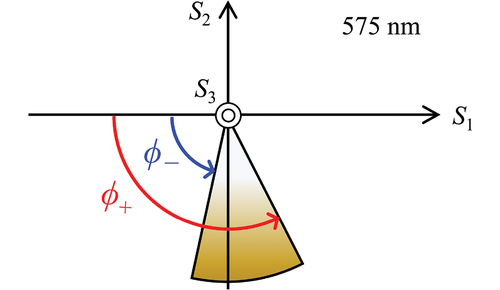
should be considered. As explained in Ref [Citation18], the angle
is represented by a periodicity of 180
in the
-plane. Because all data between 130.9 and 14.1 K, regardless of the clusters, are concentrated around
in the third and fourth quadrants, as shown schematically in , the angles of
and
can be calculated as follows: if
and
,
Figure 8. Schematic drawing of the Stokes parameters and
in the
-plane. All our experimental data for
nm between 130.9 and 14.1 K show
in the third and fourth quadrants. The definitions of
and
differ depending on the sign of
as in Equations (16) and (17).
while if and
,
However, since “’’ is a multivalued function, it is necessary to adjust
to match the angle as shown in . Using EquationEquation (14)
(14)
(14) , EquationEquations (16)
(16)
(16) and (Equation17
(17)
(17) ) can be rewritten as follows:
Because the angle has the
periodicity, to avoid “
’’ singularities, the relationship between the Stokes parameters and
expressed as
where is the sum of the differences in the Stokes parameters at the
-th
point. In our birefringence imaging measurements, the variables
at all pixels are identified simultaneously in a single measurement, assuming the condition
for the respective pixels. Furthermore, as mentioned in
2.1, the incident light was set to
[Citation16]. Therefore, the measurement error of
in a single measurement at a certain
is important, and the Bayesian
-series estimation based on linear statistics was performed in a simplified manner using EquationEquation (19)
(19)
(19) . The convergence of the MCMC simulations was assessed using trace plots and Gelman – Rubin statistics [Citation64]. The trace plots showed effective mixing and overlap between the chains. As detailed in Supplementary materials, the effective sample size (
) derived from the MCMC simulations exceeded
40% of the total sample size, which consisted of 1,584,000 iterations. An
lower than 10% of the total iterations typically indicates a high degree of autocorrelation, suggesting that the MCMC chain may not be exploring the parameter space efficiently. Conversely, our results with
well above this threshold indicate that the MCMC simulations were sufficiently efficient, with lower autocorrelation, ensuring a robust exploration of the parameter space. The Gelman – Rubin diagnostic value (
) was 1.00 for all three parameters including the log probability of the unconstrained parameters, indicating satisfactory convergence between the chains (see Supplementary materials).
shows the results of the analysis for to visually represent the posterior distributions for the MCMC simulations of
. shows a box and whisker plot of the exploration values in the fast-axis direction, expressed as
) [Citation65]. shows the probability density histogram for
for E3 and E4. The scales of the angular measures in these figures are very narrow, ranging from
to
; thus, they can be treated as linear statistics. Therefore, these figures allow a direct comparison to detect any significant differences between the four clusters. shows the five-number summary, i.e. minimum, first quartile
, median, third quartile
, and maximum, and mean for
of each cluster needed to construct the plot in . In our analysis, outliers in the box and whisker plots are identified based on a common statistical criterion involving the interquartile range (IQR) defined as
. Exploration values outside the range from
to
are considered outliers [Citation65]. This approach is widely accepted for outlier detection because it provides a balance between sensitivity to extreme values and robustness to the natural variability of the data. Although the exploration of the parameter space for
was set wide, i.e.
117–243
, both the minimum and maximum values in fell within a narrower range than the variation in the
curves shown in . In Bayesian estimation, the prior probability distribution is used to reduce the computational cost by narrowing the range of variables. However, if this range is extremely restrictive, it can limit the exploration of the parameter space, potentially leading to incomplete or biased results. Thus, it is crucial to balance the reduction in computational cost with the need for sufficient exploration. The relationship between exploration values and range limits is a key consideration in the Bayesian approach (see Supplementary materials). The difference in the mean of
between E1 and E2 is about 1.9
, and this becomes the origin of the stripe pattern along
, as shown in . To further assess the significant difference in
between E3 and E4, Cohen’s
with Hedges’ correction was calculated as
[Citation61,Citation62]. In addition, after 100,000 resamplings of the
value, the bootstrap 95% confidence interval is
. This indicates a significant difference between E3 and E4, and agrees well with the probability density histogram shown in . From
, it can be quantitatively seen that E1 and E3 form one pair and E2 and E4 form another pair in the elongated domains along
. These results confirm the successful separation of
-shape clustering with
. This Bayesian approach, although indirect, simplifies the assessment of significant differences between clusters. In addition, the stripe pattern along
, which remained ambiguous in the
-means clustering, was separated by the
-shape clustering. This may be because the
-means clustering used the absolute value of the difference between the 30.0 and 14.1 K datasets to reduce the computational cost, possibly eliminating some information in
[Citation18].
Figure 9. (a) A box and whisker plot of the exploration values of the averaged fast-axis direction, expressed as . (b) Probability density histogram for
for E3 and E4. The scales of the angular measures in these figures are highly narrow; thus, they can be treated as linear statistics.
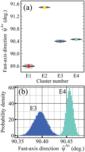
Table 2. Five-number summary (minimum, first quartile, median, third quartile, and maximum) and mean of exploration values of fast-axis direction for respective clusters expressed as .
4.3. Hierarchical Bayesian temperature-series estimation
From previous studies of stress-induced ferroelectricity in SrTiO, it was found that both
and
increase with increasing stress [Citation19–22]. As reported in Ref [Citation16], the value of
also increases due to increased stress and/or strain due to the photoelastic effect. The purpose of this study is to clarify the distribution of stress and/or strain from
and the distribution of the ferroelectric state from
on a pixel-by-pixel basis. The previous method typically estimates the phase transition temperature from the intersection of two straight lines on the
curve using the least squares method [Citation16–18]. However, this method is sensitive to outliers and cannot account for measurement errors due to its point estimation methodology. To ensure consistent quality of analysis across all 42,280 different
-series data, we used hierarchical Bayesian
-series estimation. This fits individual models at lower levels, guided by constraints from the higher-level model. In other words, as shown in , the phase transition temperatures were estimated for each pixel while simultaneously estimating the overall phase transition temperature within the cluster.
Figure 10. (a) Representation of the hierarchical Bayesian -series estimation for phase transition temperatures at each pixel (
and
for
–42,280) and for the entire cluster (
and
for
–4). Schematic representation of the model Hamiltonian used for the hierarchical Bayesian
-series estimation of (b)
and (c)
from the
curve at position a3.
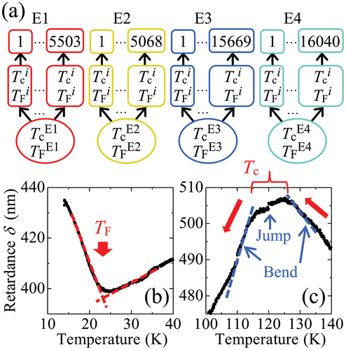
Because the estimation of is a more intuitive treatment than that of
, the hierarchical Bayesian
-series estimation method for
is explained first. For the
estimation, we used the intersection of two straight lines, as shown schematically in . The notations
for the pixels (
) and
for the clusters (
) denote the ferroelectric transition temperature at the
-th pixel and as a whole in the E
cluster, respectively. However, because the number
is a sequential number unrelated to the cluster number
, it is necessary to count only the skipped number
belonging to each cluster based on the
-shape clustering result shown in . As shown in , a positive slope is assumed for
(the paraelectric region), and a negative slope is assumed for
(the ferroelectric region). For this analysis, the
data at 575 nm from 40.0 to 14.1 K were entered into the machine learning in their measured order. To reduce the computational cost, the
curves were smoothed by averaging every two
points for the
values, resulting in 159 points with an interval of approximately 0.17 K between 40.0 and 14.1 K. In addition, the smoothed
curve at the
-th pixel was standardized, denoted as
, where
is the
-th
point. Standardization makes it easier to define a more appropriate prior probability distribution because all data can be treated on the same scale without affecting the estimation of
and
. After extensive optimization, the prior probability distribution was defined as follows:
where is the Cauchy distribution varying
with median
and scale parameter
. Compared with the normal distribution, the heavier tails of the Cauchy distribution are more robust to outliers, thereby providing a more flexible and tolerant approach to modeling errors in data with potential anomalies. The range limits for
and
are set to
The probability distributions for and
are broad, but
is closely related to
in EquationEquation (21)
(21)
(21) . Under these conditions, the model Hamiltonian is as follows: if
(the paraelectric state),
while if (the ferroelectric state),
where is the temperature at the
-th
point, i.e.
K,
,
K. Unlike EquationEquation (13)
(13)
(13) , EquationEquations (24)
(24)
(24) and (Equation25
(25)
(25) ) use linear statistics to address the errors in
because we estimate the intersection of two straight lines on the linear graph.
Below 40.0 K, the displacement of the sample position is negligible because the stress apparatus underwent sufficient thermal shrinkage. Therefore, as shown in , the measurement error corresponding to could be small. The parameters
and
in EquationEquations (24)
(24)
(24) and (Equation25
(25)
(25) ) were constrained to
(a positive slope) and
(a negative slope), respectively, but the parameter
was not constrained. The MCMC simulations were performed with different random initial values for 20,000 iterations each over eight chains, with the first 1,000 being the warm-up period. As detailed in the Supplementary materials, the
derived from the MCMC simulations exceeded
40% of the total sample size, which consisted of 152,000 iterations. For convergence diagnostics, the Gelman – Rubin statistics were computed for seven parameters, including the log probability of the unconstrained parameters associated with the estimation of
and
, and
of all variables and pixels remained below 1.05, indicating satisfactory convergence (see Supplementary materials).
To estimate , the structural phase transition temperature at each pixel,
(
), and in the E
cluster,
(
), were determined similar to
. shows that the
peak at
120 K has a large width and significant jump and bend, making it difficult to use two straight lines to identify the intersection. Despite the computational burden, we could detect a trend change from increasing to decreasing by comparing the values of
at the current
and a previous
. This approach could be called ‘Bayesian temperature-series change point detection’ as it is derived from the time-series analysis [Citation33]. In this method, the order of the
-series data and the uniformity of the
intervals may affect the estimation results; however, the data were entered in their measured order without any correction. In , several types of slopes can be observed around the peak top. In this study, by setting a wide distribution of measurement error, we detected temperatures that entered a strongly decreasing trend (see Supplementary materials). The
curve between 149.7 and 100.1 K for each pixel was smoothed by averaging every eight
points, resulting in a series of 74 points and an interval of approximately 0.68 K. Although the
interval of the
estimate is larger than that of the
estimate, this discrepancy is not a problem because the
intervals are approximately the same when normalized by the respective phase transition temperatures based on the scaling laws [Citation1]. Furthermore, the smoothed
curve between 149.7 and 100.1 K at the
-th pixel was standardized and denoted as
. To explore the parameter space more independently, we defined the structural phase transition temperatures as follows:
where is the deviation between
and
. Post optimization, the prior probability for the MCMC simulations was defined as follows:
We set a wider range for but a narrower range for
. Preliminary runs indicated that exploring
does not significantly affect the estimation of
, as
is uniformly distributed over the substrate (see Supplementary materials). To minimize the risk of converging to local minima, we systematically reduced the range limit while closely monitoring the posterior probability distribution. The final exploration range was then determined using EquationEquation (28)
(28)
(28) , considering the balance between the computational time and accuracy. Under these conditions, the model Hamiltonian is as follows: if
(the cubic phase),
while if (the tetragonal phase),
where and
are the standardized
curves at the
-th pixel for the
-th and (
)-th
points, respectively. The measurement error
was set to a distribution that was sufficiently wide to be regarded as an essentially uniform distribution. The parameters
and
in EquationEquations (29)
(29)
(29) and (Equation30
(30)
(30) ) are assumed as
(an increasing trend) and
(a decreasing trend), respectively. The MCMC simulations were performed with different random initial values for 20,000 iterations each over four chains, with the first 1,000 as the warm-up period. As detailed in the Supplementary materials, the
derived from the MCMC simulations exceeded
20% of the total sample size, which consisted of 76,000 iterations. The convergence diagnostics used the Gelman – Rubin statistics for 81 parameters, including the log probability of the unconstrained parameters associated with the estimation of
and
, and
of all variables and pixels were below 1.05, indicating satisfactory convergence (see Supplementary materials).
4.4. Analysis for each pixel
shows the results of the exploration values for , expressed as
and
, to visually represent the posterior distributions for the MCMC simulations. shows a box and whisker plot of
(
). presents a five-number summary and the mean required for constructing this plot. The exploration of the parameter space for
is set wide in EquationEquation (27)
(27)
(27) ; therefore, the minimum and maximum values are widely scattered, but their ranges are sufficiently narrower than their limits. No significant differences in
were observed between clusters. shows a probability density histogram for
, summed over the exploration values at all pixels in each cluster. Although this plot is unsuitable for understanding the characteristics of
on a pixel-by-pixel basis, the distribution of
showed no significant differences between clusters. We calculated the Pearson correlation coefficient (
) to examine the relationship between
(the higher level) and
(the lower level). Because the coefficient
measures the relative relationship between two groups, changes in the scale or position of the variables do not affect the strength or direction of the correlation. In general, a linear relationship is considered strong when
, moderate when
, and weak or indicative of almost no correlation when
[Citation61]. For the correlation between
and
, the coefficient
exceeds 0.94 for all pixels, because the exploration of
did not affect the estimation of
. This indicates a uniform distribution of
over the substrate (see Supplementary materials). shows the distribution of the mean of
for all pixels, which appears almost uniform. Although the standard deviation is often used when discussing the degree of distribution, it does not accurately represent the characteristics of the distribution if the dataset has an asymmetric distribution or numerous outliers. Furthermore, to compare the distribution of
and
, we must use indicators that can be analyzed at different scales. Therefore, a quantitative assessment of the variation in the mean of
is facilitated by , which presents the calculations of median absolute deviation (MAD) and coefficient of variation (CV) [Citation65]. In addition, the bootstrap 95% confidence interval is also shown after 100,000 resamplings. The MAD metric, which indicates the median deviation from the median, provides a robust assessment of data scatter that is less sensitive to outliers. The CV metric, which is the standard deviation divided by the mean, reflects the relative variation. These metrics are useful for comparing datasets of different scales. From , the MAD shows that the variation is smaller for E1 and E2 than for E3 and E4, but the difference is small. Furthermore, the CV shows that the standard deviation is estimated to be approximately 0.1
0.2% of the mean; thus, the overall variation in the mean of
is almost quantitatively uniform.
Figure 11. (a) A box and whisker plot of exploration values of structural phase transition temperatures in clusters, expressed as ,
,
, and
. (b) Probability density histogram of the sum of the exploration values of
for each pixel when structural phase transition temperatures at a pixel are expressed as
. All histograms overlap. (c) Distribution plot of the mean of
.
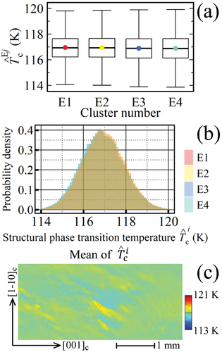
Table 3. Five-number summary and mean of exploration values of the structural phase transition temperatures for respective clusters expressed as ,
,
, and
.
Table 4. Median absolute deviation (MAD) and coefficient of variation (CV) in the distribution of the mean of and
for respective clusters. The upper panel of each column displays the values of MAD and CV, whereas the lower panel provides the bootstrap 95% confidence intervals for them.
shows the results of the exploration values for , represented as
and
. shows a box and whisker plot of
(
). provides a five-number summary and the mean required for constructing this plot. For E1 and E2,
and
are scattered on the high-
side; thus, the mean is more than 0.5 K above the median and the IQR is more than twice as large as for E3 and E4. shows a probability density histogram for
, summed over the exploration values at all pixels in each cluster. In E1 and E2, the histograms show 3–4 peaks, indicating a mixture of several groups. Conversely, for E3 and E4, the histograms are concentrated on the lower-
side. For the correlation between
and
in each cluster, the coefficients
are widely scattered within
, although the means of
in the respective clusters are 0.25–0.31 (see Supplementary materials). This indicates that the lower-level estimation is successfully performed for each pixel, while being restricted by the higher-level estimation of the entire cluster. shows the distribution of the mean of
. The MAD and CV, and their bootstrap 95% confidence intervals after 100,000 resamplings were calculated to evaluate the distributions of the mean of
and are shown in . The MAD results show that the distributions of the mean of
from the median are more than twice as wide for E1 and E2 than for E3 and E4. The CV results show that the standard deviation of the mean of
is approximately 8% of the mean for E1 and E2, and approximately 4% of the mean for E3 and E4. For both metrics, E1 and E2 are a pair and E3 and E4 are another pair. shows Cohen’s
with Hedges’ correction of distributions of
and the bootstrap 95% confidence interval after 10,000 resamplings of
for each pair of clusters to assess significant differences. Consequently, significant differences exist between the clusters, except for the pair E1 and E2 and pair E3 and E4. This is consistent with the
curves shown in .
Figure 12. (a) A box and whisker plot of exploration values of ferroelectric phase transition temperatures in clusters, expressed as ,
,
, and
. (b) Probability density histogram of the sum of the exploration values of
for each pixel when structural phase transition temperatures at a pixel are expressed as
. The histograms for E1 and E2 overlap, and those for E3 and E4 overlap. (c) Distribution plot of the mean of
.
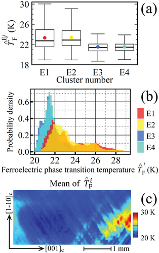
Table 5. Five-number summary and mean of exploration values of the ferroelectric phase transition temperatures for respective clusters expressed as ,
,
, and
.
Table 6. Cohen’s with Hedges’ correction of the distributions of the exploration values
in two combinations within E1, E2, E3, and E4. Because the sign of the
value is insignificant, the upper panel of each column displays the absolute value of
, whereas the lower panel details the bootstrap 95% confidence intervals for
.
From Ref [Citation18]. the larger regions indicate the stress and/or strain concentration. On the basis of linear relationship between stress and
expressed as EquationEquation (1)
(1)
(1) , the stress distribution was also considered. By uniformly subtracting 105 K from the means of
in clusters, the standard deviations remain unchanged, while the mean and median are changed. Therefore, the MADs remain constant, but the CVs change, and the relative relationship between the CVs could change. However, if the means of
in clusters are multiplied by the same factor, the relationship between the MADs does not change as the same coefficients are multiplied for them. Comparing the MADs, the relationship of the means of
between clusters is opposite to that of the means of
. In Ref [Citation16], we have already proposed evaluating the stress and/or strain distribution using
caused by the photoelastic effect. The distributions of
and
at 130.9 K in and those at 14.1 K in of Ref [Citation16]. are similar to the distribution of the mean of
in . To evaluate the similarity quantitatively, shows the heat maps of the coefficient
between
,
, means of
, and means of
. Concerning the correlations between the means of
and
, there are moderate correlations for E1 but weak or no correlations for E2–E4. Furthermore, for the relationship between
and the means of
, there are moderate correlations for E1 and E2, but almost no correlations for E3 and E4 at 130.9 K, whereas there are strong correlations for E1 and E2, and moderate correlations for E3 and E4 at 14.1 K. Contrary to our expectation, we could not find any pair of variables showing a strong correlation for E3 and E4, despite almost uniform stress and/or strain. Consequently, the stress and/or strain distribution could be better estimated from
or the mean of
than from the mean of
.
Figure 13. Heat maps for each cluster of Pearson correlation coefficients () between
,
, mean of
and mean of
at (a) 130.9 K and (b) 14.1 K.
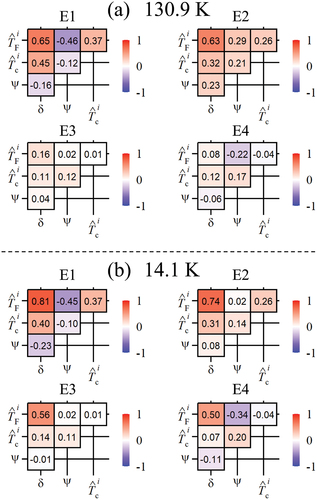
Finally, we speculate why the correlation is stronger for E1 and E2 than for E3 and E4. If the Pockels effect causes an increase in the curve below
, the coefficient
should be stronger for E3 and E4 than for E1 and E2 because of the less disordered crystal orientation. Meanwhile, considering the photoelastic effect, we can assume a strong linear relationship between the local stress and/or strain and
. Although it is not easy to distinguish between these effects experimentally, we hypothesize that flexoferroelectricity is induced by local strain, which is an interesting concept [Citation66], but it borders on speculative territory in this study. At zero electric field, the ensemble average of the normal spontaneous polarization within a pixel (
10
10
m
) is very small, whereas that of the flexoferroelectric polarization may be large because the strain has already biased it in a certain direction. If this scenario is true, flexoferroelectric polarization would be generated locally for E1 and E2 in addition to the normal ferroelectric polarization distributed throughout the substrate. This hypothesis can be tested by applying electric fields at various
. For example, the flexoferroelectricity is bound to the lattice distortions; therefore, different electric field dependencies may emerge within the substrate. In the future, to confirm the nonlinear relationship between
,
, and stress and/or strain, we will also apply machine learning using nonlinear models such as decision trees and random forests to unravel the complex dynamics governing the flexoferroelectricity and normal ferroelectricity.
5. Conclusion
In this study, the stress-induced ferroelectric domains elongated along in SrTiO
were investigated by combining machine learning and statistics to extract deep insights from large
-series birefringence imaging data. After applying the advanced preprocessing to characterize the spatial information of the
-series data, we first performed the multivariate
-shape clustering method focused on the shape similarity of the
dependencies. This result showed that a large spontaneous polarization appears for E1 and E2 owing to stress and/or strain concentration. Furthermore, hierarchical Bayesian
-series estimation was used to ensure consistent analysis of 42,280-pixel
-series data to estimate
and
for each pixel as constrained by the overall
and
in the cluster. For the means of
, the uniform distribution over the substrate is strongly supported. Furthermore, the means of
for E1 and E2 are widely scattered to the high-
side. The higher region coincides well with the stress and/or stress concentration regions. Consequently, the hierarchical Bayesian
-series estimation strongly supports the
-shape clustering results. Based on the correlation coefficients for E1 and E2, a strong correlation exists between
and the means of
, but the correlations become moderate for E3 and E4. Because of the weak or no correlation between the means of
and
, it is difficult to deduce the distribution of stress and/or strain from these means. Our multistep
-series analysis method has proven considerably useful for studying critical phenomena near phase transition temperatures. Further development of
-series analysis is essential for the widespread use of machine learning in condensed matter physics.
Supplemental Material
Download PDF (33.8 MB)Disclosure statement
No potential conflict of interest was reported by the author(s).
Supplementary material
Supplemental data for this article can be accessed online at https://doi.org/10.1080/27660400.2024.2342234
Additional information
Funding
References
- Yeomans YM. Statistical mechanics of phase transitions. Oxford Science Publications; 1992.
- Gautam R, Vanga S, Ariese F, et al. Review of multidimensional data processing approaches for Raman and infrared spectroscopy. EPJ Techn Instrum. 2015;2(1):8. doi: 10.1140/epjti/s40485-015-0018-6
- Mueller T, Kusne AG, Ramprasad R. Machine learning in materials science: recent progress and emerging applications. Rev Comput Chem. 2016;29:186–19. doi: 10.1002/9781119148739
- Rodrigues JF Jr, Florea L, Oliveira MCF. Big data and machine learning for materials science. Discover Materials. 2021;1(1):12. doi: 10.1007/s43939-021-00012-0
- Turrell G, Corset J. Raman microscopy: developments and applications. London: Academic Press; 1996.
- Lieber CM. Nanoscale science and technology: building a big future from small things. Mater Res Bull. 2003;28(7):486–491. doi: 10.1557/mrs2003.144
- Meyer E. Scanning probe microscopy and related methods. Beilstein J Nanotechnol. 2010;1:155–157. doi: 10.3762/bjnano.1.18
- Fleming A. Dual-stage vertical feedback for high-speed scanning probe microscopy. IEEE Trans Control Syst Technol. 2011;19(1):156–165. doi: 10.1109/TCST.2010.2040282
- Casola F, Sar T, Yacoby A. Probing condensed matter physics with magnetometry based on nitrogen-vacancy centres in diamond. Nat Rev Mater. 2018;3(1):17088. doi: 10.1038/natrevmats.2017.88
- Uemura Y, Matsuoka S, Tsutsumi J, et al. Birefringent field-modulation imaging of transparent ferroelectrics. Phys Rev Appl. 2020;14(2):024060. doi: 10.1103/PhysRevApplied.14.024060
- Laskar MDAR, Celano U. Scanning probe microscopy in the age of machine learning. APL Mach Learn. 2023;1(4):041501. doi: 10.1063/5.0160568
- Trebbia P, Bonnet N. EELS elemental mapping with unconventional methods I. theoretical basis: image analysis with multivariate statistics and entropy concepts. Ultramicroscopy. 1990;34(3):165–178. doi: 10.1016/0304-3991(90)90070-3
- Bonnet N, Brun N, Colliex C. Extracting information from sequences of spatially resolved EELS spectra using multivariate statistical analysis. Ultramicroscopy. 1999;77(3–4):97–112. doi: 10.1016/S0304-3991(99)00042-X
- Muto S, Yoshida T, Tatsumi K. Diagnostic nano-analysis of materials properties by multivariate curve resolution applied to spectrum images by S/TEM-EELS. Mater Trans. 2009;50(5):964–969. doi: 10.2320/matertrans.MC200805
- Shiga M, Tatsumi K, Muto S. Sparse modeling of EELS and EDX spectral imaging data by nonnegative matrix factorization. Ultramicroscopy. 2016;170:43–59. doi: 10.1016/j.ultramic.2016.08.006
- Manaka H, Uetsubara K, Korogi S, et al. Microscopic observation of ferroelectric and structural phase transitions in SrTiO3 under uniaxial stress using birefringence imaging techniques. J Phys Soc Jpn. 2022;91(8):084704. doi: 10.7566/JPSJ.91.084704
- Manaka H, Uetsubara K, Miura Y. Stress-induced ferroelectricity in quantum paraelectric SrTiO3 observed by birefringence imaging. JPS Conf Proc. 2023;38:011112.
- Toyoda K, Manaka H, Miura Y. Improvements of birefringence imaging techniques to observe stress-induced ferroelectricity in SrTiO3 based on K-means clustering with circular statistics. Sci Technol Adv Mater Meth. 2023;3(1):2278322. doi: 10.1080/27660400.2023.2278322
- Müller KA, Berlinger W, Slonczewski JC. Order parameter and phase transitions of stressed SrTiO3. Phys Rev Lett. 1970;25(11):734. doi: 10.1103/PhysRevLett.25.734
- Burke WJ, Pressley RJ. Stress induced ferroelectricity in SrTiO3. Solid State Commun. 1971;9(3):191–195. doi: 10.1016/0038-1098(71)90115-3
- Uwe H, Sakudo T. Stress-induced ferroelectricity and soft phonon modes in SrTiO3. Phys Rev B. 1976;13(1):271–286. doi: 10.1103/PhysRevB.13.271
- Fujii Y, Uwe H, Sakudo T. Stress-induced quantum ferroelectricity in SrTiO3. J Phys Soc Jpn. 1987;56(6):1940–1942. doi: 10.1143/JPSJ.56.1940
- Ohtomo A, Hwang HY. A high-mobility electron gas at the LaAlO3/SrTiO3 heterointerface. Nature. 2004;427(6973):423–426. doi: 10.1038/nature02308
- Honig M, Sulpizio JA, Drori J, et al. Local electrostatic imaging of striped domain order in LaAlO3/SrTiO3. Nat Mater. 2013;12(12):1112. doi: 10.1038/nmat3810
- Lee PW, Singh VN, Guo GY, et al. Hidden lattice instabilities as origin of the conductive interface between insulating LaAlO3 and SrTiO3. Nat Commun. 2016;7(1):12773. doi: 10.1038/ncomms12773
- Su CP, Singh AK, Wu TC, et al. Impact of strain-field interference on the coexistence of electron and hole gases in SrTiO3/LaAlO3/SrTiO3. Phys Rev Mat. 2019;3:075003. doi: 10.1103/PhysRevMaterials.3.075003
- Bishop CM. Pattern recognition and machine learning (information science and statistics). Springer; 2006.
- Vasudevan RK, Tselev A, Baddorf AP, et al. Big-data reflection high energy electron diffraction analysis for understanding epitaxial film growth processes. ACS Nano. 2014;8(10):10899–10908. doi: 10.1021/nn504730n
- Provence SR, Thapa S, Paudel R, et al. Machine learning analysis of perovskite oxides grown by molecular beam epitaxy. Phys Rev Mater. 2020;4(8):083807. doi: 10.1103/PhysRevMaterials.4.083807
- Gliebe K, Sehirlioglu A. Distinct thin film growth characteristics determined through comparative dimension reduction techniques. J Appl Phys. 2021;130(12):125301. doi: 10.1063/5.0059655
- Yoshinari A, Iwasaki Y, Kotsugi M, et al. Skill-agnostic analysis of reflection high-energy electron diffraction patterns for Si(111) surface superstructures using machine learning. Sci Technol Adv Mater Meth. 2022;2(1):162–174. doi: 10.1080/27660400.2022.2079942
- Senin P. Dynamic time warping algorithm review. Inf Comput Sci Dep Univ Hawaii Manoa Honol. USA. 2008;855(1–23):40.
- Box GEP, Jenkins GM, Reinsel GC, et al. Time series analysis: forecasting and control. 5th ed. Wiley; 2015.
- Paparrizos J, Gravano L. K-shape: efficient and accurate clustering of time series. SIGMOD Rec. 2016;45(1):69–76. doi: 10.1145/2949741.2949758
- Mohammad-Djafari A, Féro O. Bayesian approach to change points detection in time series. Int J Imaging Syst Tech. 2007;16(5):215–221. doi: 10.1002/ima.20080
- Iwamitsu K, Aihara S, Okada M, et al. Bayesian analysis of an excitonic absorption spectrum in a Cu2O thin film sandwiched by paired MgO plates. J Phys Soc Jpn. 2016;85(9):094716. doi: 10.7566/JPSJ.85.094716
- Cowley RA. Lattice dynamics and phase transitions of strontium titanate. Phys Rev. 1964;134(4A):A981. doi: 10.1103/PhysRev.134.A981
- Courtens E. Birefringence of SrTiO3 produced by the 105°K structural phase transition. Phys Rev Lett. 1972;29(20):1380. doi: 10.1103/PhysRevLett.29.1380
- Cowley RA. The phase transition of strontium titanate. Phil Trans R Soc A. 1996;354(1720):2799–2814. doi: 10.1098/rsta.1996.0130
- Haeni JH, Irvin P, Chang W. Room-temperature ferroelectricity in strained SrTiO3. Nature. 2004;430(7001):758. doi: 10.1038/nature02773
- Kim YS, Kim DJ, Kim TH, et al. Localized electronic states induced by defects and possible origin of ferroelectricity in strontium titanate thin films. Appl Phys Lett. 2007;91(4):042908. doi: 10.1063/1.3139767
- Iglesias L, Sarantopoulos A, Magén C, et al. Oxygen vacancies in strained SrTiO3 thin films: formation enthalpy and manipulation. Phys Rev B. 2017;95(16):165138. doi: 10.1103/PhysRevB.95.165138
- Hashimoto T, Nishimatsu T, Mizuseki H, et al. Ab initio study of strain-induced ferroelectricity in SrTiO3. Jpn J Appl Phys. 2005;44(9S):7134. doi: 10.1143/JJAP.44.7134
- Antons A, Neaton JB, Rabe KM, et al. Tunability of the dielectric response of epitaxially strained SrTiO3 from first principles. Phys Rev B. 2005;71(2):024102. doi: 10.1103/PhysRevB.71.024102
- Ni L, Liu Y, Song C, et al. First-principle study of strain-driven phase transition in incipient ferroelectric SrTiO3. Physica B. 2011;406(21):4145. doi: 10.1016/j.physb.2011.08.018
- Ong PV, Lee J. Strain dependent polarization and dielectric properties of epitaxial BaTiO3 from first-principles. J Appl Phys. 2012;112(1):014109. doi: 10.1063/1.4736375
- Watanabe Y. Ferroelectricity of stress-free and strained pure SrTiO3 revealed by ab initio calculations with hybrid and density functionals. Phys Rev B. 2019;99(6):064107. doi: 10.1103/PhysRevB.99.064107
- Azzam RM, Bashara NM. Ellipsometry and polarized light. North Holland: Amsterdam; 1977.
- Manaka H, Yagi G, Miura Y. Development of birefringence imaging analysis method for observing cubic crystals in various phase transitions. Rev Sci Instrum. 2016;87(7):073704. doi: 10.1063/1.4958662
- Manaka H, Fukuda T, Miura Y. Birefringence imaging measurements on various structural phase transitions in (CnH2n+1NH3)2MnCl4 with n=1,2, and 3 using multiple wavelengths. J Phys Soc Jpn. 2016;85(12):124701. doi: 10.7566/JPSJ.85.124701
- Manaka H, Nozaki H, Miura Y. Microscopic observation of ferroelectric domains in SrTiO3 using birefringence imaging techniques under high electric fields. J Phys Soc Jpn. 2017;86(11):114702. doi: 10.7566/JPSJ.86.114702
- Manaka H, Nozaki H, Miura Y. Development of birefringence imaging techniques under high electric fields. J Phys Conf Ser. 2018;969:012119. doi: 10.1088/1742-6596/969/1/012119
- Manaka H, Sasaki Y, Miura Y. Re-examination of successive structural phase transitions in (C3H7NH3)2CuCl4 using birefringence imaging and electron paramagnetic resonance spectroscopy. J Phys Soc Jpn. 2017;86(11):114710. doi: 10.7566/JPSJ.86.114710
- Miura Y, Okumura K, Fukuda T, et al. Observation of ferroelastic domains in layered magnetic compounds using birefringence imaging. J Phys Conf Ser. 2018;969:012153. doi: 10.1088/1742-6596/969/1/012153
- Manaka H, Okumura K, Tokunaga K, et al. Observations of successive local-structure and ferroelectric phase transitions in (C2H5NH3)2CuCl4 using birefringence imaging and electron paramagnetic resonance spectroscopy. J Phys Soc Jpn. 2022;91(11):114701. doi: 10.7566/JPSJ.91.114701
- Miura Y, Ibushi R, Manaka H. Observation of ferroelectricity in two-dimensional antiferromagnet (C2H5NH3)2CuCl4 using birefringence imaging techniques. JPS Conf Proc. 2023;38:011142. doi: 10.7566/JPSCP.38.011142
- Fisher NI. Statistical analysis of circular data. Cambridge University Press; 1993.
- Pewsey A, Neuhauser M, Ruxton GD. Circular statistics in R. Oxford University Press; 2014.
- Manaka H, Tateishi K, Miura Y. Real-space imaging by magnetic birefringence for KNiF3 under inhomogeneous stress. J Phys Soc Jpn. 2019;88(12):124702. doi: 10.7566/JPSJ.88.124702
- Schubert E. Stop using the elbow criterion for K-means and how to choose the number of clusters instead. ACM SIGKDD Explorations Newsl. 2023;2(1):36–42. doi: 10.1145/3606274.3606278
- Cohen J. Statistical power analysis for the behavioral sciences. 2nd ed. Routledge; 1988.
- Hedges LV, Olkin I. Statistical methods for meta-analysis. Academic Press; 1985.
- Durlak JA. How to select, calculate, and interpret effect sizes. J Pediatr Psychol. 2009;34(9):917–928. doi: 10.1093/jpepsy/jsp004
- Gelman A, Carlin JB, Stern HS. Bayesian data analysis. Chapman and Hall/CRC; 2013.
- Tukey JW. Exploratory data analysis. Pearson Education, Ltd.; 1977.
- Das S, Wang B, Paudel T, et al. Enhanced flexoelectricity at reduced dimensions revealed by mechanically tunable quantum tunnelling. Nature Commun. 2019;10(1):537. doi: 10.1038/s41467-019-08462-0