
 ?Mathematical formulae have been encoded as MathML and are displayed in this HTML version using MathJax in order to improve their display. Uncheck the box to turn MathJax off. This feature requires Javascript. Click on a formula to zoom.
ABSTRACT
For classifying and modeling properties of crystalline materials in terms of structure, a three-step workflow with (1) generation of structure feature vectors, (2) evaluation of distances among the feature vectors as a measure of similarity in structure, and (3) mapping of each structure in a low-dimensional space with principal components using dimension reduction is proposed. The obtained distance and resulting principal components are useful for classifying similar crystal structures for a given set of materials systems and for constructing descriptors in machine-learning analyses of properties. The eigenvector of the principal components indicates which part of the original structure feature vector is contained as important information. Examples are demonstrated for classification and property modeling of AlO
polymorphs including amorphous structures and of the alloy configurations of Si-doped LaFe
compounds.
GRAPHICAL ABSTRACT
IMPACT STATEMENT
Crystal structure map constructed from the feature of structures by a dimension-reduction technique for classification and modeling for a group of related materials such as polymorphs, alloys, and doped systems.
1. Introduction
Today, a wealth of materials information is being generated, collected, and accumulated, experimentally, theoretically, and computationally. One of the current hot issues in materials research is materials discovery assisted by data-science approach with the information [Citation1]. For materials exploration and design, it is important to know in advance where each existing materials system is positioned in a map and more basically how the coordinate system of the map is defined for a given set of materials group. This raises a novel concept ‘materials map’ [Citation2]. Since the materials space is super high dimensional, the key to the materials map for a concrete target materials system is to extract appropriate features which define the low-dimensional axes of the map like the latitude and longitude of the ordinary geological maps.
Atomic configuration in space simply called structure is the most fundamental attribute of molecular and condensed matter systems, especially crystalline materials, and determines the Hamiltonian for electronic states together with their composition under the Born-Oppenheimer approximation [Citation3]. Our understanding of materials property is often based on its correlation with the structure. Usually, the huge sum of structure types exist in nature and can be classified by using symmetry in point group or space group (SG), that is ingeniously connected to the electronic states and related electronic properties.
For example, the electronic state of a condensed matter is often described by analyzing the symmetry of local structure around the target atom in terms of orbital splitting and hybridization. The electronic band structure of a crystalline system obeys its translational symmetry with the definition of the Brillouin zone on the basis of the Bloch theorem. In general, however, the structure dependence of the obtained electronic state and resulting properties is not so easily understood because of high-dimensionality in the structure space. With the desired structure map, the low-dimensional coordinates should classify huge related types of structure and the corresponding axes should provide structure descriptors for materials modeling following.
A common language is needed to start the analysis of the huge number of structures for a given general materials group. It should contain all the necessary but unambiguous information of the structure we investigate. In crystalline materials, the components of structural information are uniquely described with the crystallographic information framework (CIF) defined by the dictionary CoreCIF [Citation4] established by International Union of Crystallography (IUCr) [Citation5]. Most of the crystallographic databases such as ICSD [Citation6], COD [Citation7], and AtomWork [Citation8] adopt the CIF format requisite for structure data standardization. Some crystallographic visualization tools also accept the CIF format data [Citation9,Citation10].
Recently, accelerated by automated high-throughput computations with first-principles density-functional-theory (DFT) electronic structure calculation methods, computational materials databases and archives containing optimized, predicted, and designed crystal structure information compatible with CIF have been constructed like Materials Project [Citation11], NOMAD [Citation12], OQMD [Citation13], AFLOW [Citation14] and etc., forming big data on crystal structures continuously growing with the experimental structure databases. To understand materials properties associated with structure for further development and deployment, it may be indispensable and worthwhile to extract important features in structure for a given target group of materials. Generally, crystal structure consists of high-dimensional information and a dimensional reduction technique is required for the purpose. In this study, a workflow to draw such important features by using a dimension-reduction technique is proposed and demonstrated for some examples.
Obtained low-dimensional features of crystal structure can be used for classifying the structures (clustering as a data-science term) among the related materials systems and also for machine-learning modeling of structure-associated electronic properties of materials. In addition, a simple technique to create possible configurational structures by substituting atomic sites of a materials system with different elements in all combinational degrees of freedom is proposed for applications to alloy and impurity problems with supercell models.
2. Methods
A three-step procedure starting from a set of the CIF files of the target crystal systems for mapping the mutual position of each crystal structure in a low-dimensional space is described in the following sub-sections. Moreover, a generation method of structures with possible required configurations for a given set of compositions is explained in connection with the three-step workflow. The whole structure of the workflow is shown in .
Figure 1. Three-step workflow described in the present study. Capital italic name expresses each detailed procedure, CIF2ESC: conversion from a CIF file to electronic-structure-calculation data with output of fingerprint as structure feature for post structure analyses; DISTANCE: evaluation of distances between structure feature vectors; DISTANCE_DISTRIBUTION: calculation of distance distribution; DIAGNOSIS: extraction of inequivalent structures; CMDS: classical multidimensional scaling; PCEV: calculation of principal component eigenvectors; PROJECTION: projection of an arbitrary structure on the dimension-reduced map; ATLS: generation of atom-type list; FINDSYM: space-group finder
: Ref [Citation15,Citation16]. Open and solid (and dotted) arrows denote data transfers between the steps and inside each step, respectively. Dotted arrow is applicable if necessary.
![Figure 1. Three-step workflow described in the present study. Capital italic name expresses each detailed procedure, CIF2ESC: conversion from a CIF file to electronic-structure-calculation data with output of fingerprint as structure feature for post structure analyses; DISTANCE: evaluation of distances between structure feature vectors; DISTANCE_DISTRIBUTION: calculation of distance distribution; DIAGNOSIS: extraction of inequivalent structures; CMDS: classical multidimensional scaling; PCEV: calculation of principal component eigenvectors; PROJECTION: projection of an arbitrary structure on the dimension-reduced map; ATLS: generation of atom-type list; FINDSYM ∗: space-group finder ∗: Ref [Citation15,Citation16]. Open and solid (and dotted) arrows denote data transfers between the steps and inside each step, respectively. Dotted arrow is applicable if necessary.](/cms/asset/3f862b2b-a1c2-4ad0-8c70-da4a5d33f2f9/tstm_a_2355860_f0001_b.gif)
2.1. STEP-1: Feature vector of crystal structure (abbreviated as CIF2ESC)
Crystal structure is the starting point of the present analysis and we assume that the detailed information for a set of materials systems is given with the CIF format. To consider a feature for a general structure, one should define a vector that is simple, tractable, translationally and rotationally invariant to treat, and often possibly highly dimensional to distinguish. Coordination number is the simplest information of local structure around a particular atomic site in a crystal. A cutoff distance to determine the nearest neighbor (NN) is rather subjective and not well defined for general structures. Radial distribution function (RDF) contains complete pair-wise structure information within a given radius and is directly measurable in extended x-ray absorption fine structure (EXAFS) experiments. An extension of RDF to more than pair correlations may be possible like cluster expansion [Citation17].
Oganov and Valle [Citation18] have proposed -fingerprint as a structure feature defined for an
element pair of a system as
where is the
-th site of element
,
is the distance between
and
,
is the number of sites of
in cell, and
is the volume of unit cell. In EquationEquation (1)
(1)
(1) , the first term is nothing but RDF and the second term
is introduced so that the
-fingerprint becomes short-ranged with an asymptotic behavior of
. The
function is smoothened with the Gaussian function of an appropriate broadening width
in a practical numerical process as
The -fingerprint in EquationEquation (1)
(1)
(1) is discretized as
with an interval
up to an assumed maximum radius
and by connecting all independent RDFs for
element pairs in series, a
-dimensional (
-D) vector is finally obtained in a vector form. The parameters included in the feature vector,
,
, and
, should be determined by judging the evaluation of structure distance according to user’s target system and purpose. Generally speaking,
corresponds to the resolution of RDF for distinguishing given structures. Thus, typical values of
may be about one tenths of Å taken from the NN and next nearest neighbor (NNN) distance in the compounds. Accordingly, the discretizing interval
should be smaller to some extent than
to make the resolution meaningful. The cutoff radius
should be selected about the cell size of the system. The RDF information beyond it might be redundant because of the periodicity in a model system.
The -fingerprint has been successfully used in our previous works [Citation19–21] for accelerating crystal structure prediction with the Bayesian optimization technique. Especially, some evaluations was made for investigating the efficiency of the crystal structure search with different choices of the parameters included in the
-fingerprint [Citation20]. Extensions of the
-fingerprint representing higher-order crystal structure information might be also applicable in the present scheme by including angular degrees of freedom as local many-site correlations [Citation22,Citation23].
2.2. STEP-2: Structure distance as a measure of similarity (DISTANCE and DIAGNOSIS)
Although similarity of crystal structure is not uniquely defined, let us consider feature-vector distance as a quantity to represent the similarity. The degree of the similarity can be considered in such a semi-quantitative way that two structures are equivalent if a structure distance satisfies
with a given threshold
, and a pair of two structures 1 and 2 with distance
is closer in structural similarity than another pair of 1 and 3 with distance
if the distances satisfy
. In any case,
can be determined by inspecting the distance distribution and the error bars in the structure data (typically significant figures of lattice constants and atomic coordinates.
Given two -D vectors
and
representing the feature of crystal structures, the simplest distance between them is the Euclidean distance defined as
For the present purpose, the Pearson correlation coefficient (PCC) can be another choice as a measure of structure similarity as
where denotes the average of the vector components. Since PCC is distributed within the range of
, it can be transformed into a kind of distance as
known as the Cosine distance. In the present case with the vectors given in EquationEquation (1)(1)
(1) , the Cosine distance between structures 1 and 2 is explicitly computed as
where the inner product is defined as
with a weight proportional to the pair probability
This means that the present scheme is limited to equal composition systems when comparing more than one distance. In the same way as EquationEquation (6)(6)
(6) , the Euclidean distance between structures 1 and 2 is obtained as
In high-throughput DFT calculations, a huge set of similar crystal structures are generated for a given composition. Some of them are essentially equivalent but are often judged to be different due to numerical errors or insufficient structural optimizations. The distance obtained above can be used for listing up crystallographically inequivalent structures among the structure set in a reasonable manner with a given threshold distance. This procedure may reduce the total computing time of DFT calculations and can be combined with a successive process for primitive-cell and symmetry determination. Without this, it is tempting to think of a large number of possible atomic configurations in an impurity or alloying problem that may contain many equivalent structures as we shall see in Sect. 3.2.
2.3. STEP-3(1): Structure mapping (CMDS)
For a given Euclidean or non-Euclidean distance matrix constructed from
structure sets of the
-D feature vectors
, dimension-reduced coordinates of the structures
approximated in a low
-D space can be obtained by using the multidimensional scaling (MDS) [Citation24–26]. (For clarity, the size of matrix is indicated like
when it first appears.) The MDS scheme is often called ‘dimension reduction’ in data mapping and is equivalent to principal component analysis (PCA) when Euclidean distance is applied. In MDS, the pair-wise Euclidean distance matrix
calculated using
is the closest approximation to D. The algorithm of MDS is quite simple as follows, starting with squared distance matrix
of which the components are squared values of the original distance matrix components. First, the squared distance matrix is transformed by the so-called double centering
into a matrix
as
where and
are identity matrix and identity column vector, respectively, and the superscript
stands for matrix transpose. Next, the matrix
is eigenvalue decomposed as
Here, the matrix contains the eigenvalues in the diagonal elements with zeros in the off-diagonal ones and
is the corresponding eigenvector matrix. Finally, by taking the first
positive-eigenvalue part
and
in the order from the positive-largest one, the principal components (PCs)
approximately representing the structure coordinates can be obtained as
where is the matrix of which diagonal elements are the square root of the eigenvalues as
. Then, the matrix B is approximated in the form of scalar product as
As indicated in EquationEquation (12)(12)
(12) , the deviation of the coordinates of each structure is proportional to the square-root of the eigenvalue, since the eigenvector
in EquationEquation (11)
(11)
(11) is usually taken in a unitary form. Thus, the size of the eigenvalue determines the importance of each PC obtained by the dimension reduction.
As Sibson has pointed out [Citation27], the value that we may choose can be determined by judging the magnitude of positive eigenvalues since the sum of the eigenvalues in
approximate the sum of all eigenvalues in
. This point is practically quite important and crucial when determining the number of PCs and evaluating the performance of feature vectors and distances we adopted [Citation28]. To see how much original information remains after the dimension reduction, it is convenient to check the so-called proportion defined by
Note that the summation in the numerator of EquationEquation (14)(14)
(14) is taken in the descending order starting from the positive largest eigenvalue.
2.4. STEP-3(2): Projection on map and its inverse operation (PCEV and PROJECTION)
Let us describe a way to get the eigenvector of PCs in the original -D space and to make the projection of a given new structure on the obtained low-dimensional map above, by considering the relation to PCA [Citation29]. In PCA, the data covariance matrix
is the target quantity and is maximized with a unitary matrix
and the LaGrange multiplier
as
leading to an eigenvalue problem of
Note that the coordinate matrix defined in this paper follows Borg-Groenen’s prescription [Citation25] in a transpose form of Bishop’s definition [Citation29]. By combining EquationEquation (12)
(12)
(12) , (Equation13
(13)
(13) ), and (Equation16
(16)
(16) ), the PC eigenvector
can be computed in a normalized form as
with the center coordinate of the original feature vectors as
The original coordinate matrix which is used to calculate the distance is not necessarily centered and is enforced to be so in EquationEquation (17)
(17)
(17) . By using the obtained PC eigenvector
, the projection of any arbitrary structure feature vector
in the original dimension space on the reduced
-D map can be made as
With help of the minimum-error formulation of PCA [Citation29], an inverse projection, that is the transformation of an arbitrary reduced coordinate on the map into a feature vector
in the original structure space, can be made as
Since a certain amount of information is lost due to the dimension reduction, the inverse projection can only be accomplished approximately. The projection and inverse projection procedures described above are reasonably made if the distance matrix is calculated as the Euclidean distance since MDS and PCA are rigorously equivalent. Even in non-Euclidean distance case, the procedures may possibly be carried out.
2.5. Generation of structures with all possible configurations (ATLS)
In addition to stoichiometric ordered materials, alloyed and doped impurity systems are often seen as targets in materials research. In such systems, counting all the possible configurations is crucially indispensable for optimizing materials properties. In electronic structure calculations for alloy systems, coherent-potential approximation (CPA) [Citation30–32] is usually adopted by taking single-site average of scattering path operators within the Korringa-Kohn-Rostoker (KKR) Green’s function formalism [Citation33,Citation34]. This approximation works quite well for randomly distributed alloy systems. Similar idea with supercell models has been proposed with special quasi-random structures (SQS’s) method, where the site configuration is optimized by making multiple site-correlation functions best close to those of random structure [Citation35,Citation36].
However, partially ordered or site-preference features are often seen and essential to govern the materials properties in real materials. Listing up all the possible configurational combinations is quite useful to investigate such local-site-order associated properties for a given composition with specific elements included. Such a tool is developed as ATLS. For a example, let us consider a body-centered supercell model containing eight atoms (four Fe and four Co) with BCC-base lattice structure. All the possible combinations are
70 ways. With given lattice constants, lattice centering types, atomic composition, and corresponding atomic coordinates, SG and related structural properties can be obtained by using FINDSYM software [Citation15,Citation16]. By using the workflow described above, only four structures are found to be crystallographically inequivalent (32
+12
+24
+2
) out of the 70 configurations. In the present work, crystallographically equivalent structures mean that their
-fingerprints are equivalent within the reasonable threshold and have the same SG. Interestingly, the
and
structures extracted above have the exactly same
-fingerprint within minor numerical error bars and cannot be distinguished only by the pair-wise information. This is a drawback of the present choice of the fingerprint and structure features beyond the pair-wise correlation should be included if necessary. Actually, it is not the case shown in the example of La(Fe,Si)
(see Sect. 3.2). In the case of a
primitive supercell model containing 16 atoms (eight Fe and eight Co) with BCC-base lattice structure, there are
combinations and 51 crystallographically inequivalent configurations. Similar to the case above, some configurations have the exactly same fingerprint, resulting in Citation32 independent pair-wise fingerprints. Some interesting situations may happen if the mother system contains more than one crystallographically inequivalent atomic sites, leading to a site-preference problem. Such a case will be given below in Section 3.2.
2.6. DFT calculations
All the DFT electronic structure calculations in the present study are performed with the all-electron full-potential linearized augmented-plane-wave (FLAPW) method [Citation37–39] implemented in the HiLAPW program [Citation40]. The exchange and correlation are incorporated within the Perdew-Burke-Ernzerhof form [Citation41] of the generalized gradient approximation to DFT. The energy cutoffs for wave function and potential expansions are 20 Ry and 160 Ry, respectively. A set of -centered
-point mesh with the interval of approximately 0.1 Bohr
is used to sample the Brillouin zone with the improved tetrahedron integration scheme [Citation42] in all the self-consistent-field DFT calculations.
3. Results and discussion
3.1. Classification of Al O polymorphs
There often exist several stable and metastable types of crystal structure with the same composition, called polymorph, especially in oxide systems. Silica SiO and alumina Al
O
are such most typical cases seen in materials science and engineering. For example, there are 15 different crystal structures of Al
O
found in the Materials Project site [Citation11]. One of them, mp -1,245,063 seems to be an amorphous model structure with 100 atoms in a unit cell (SG:
). In addition, another amorphous model structure including 120 atoms in a unit cell was generated by a first-principles molecular-dynamics simulation with a quenching scheme from a liquid state [Citation43]. Structural analyses on Al
O
for several different phases have been carried out in relation to their properties [Citation44–46].
A map for the AlO
structures is created by using the three-step procedure proposed above, and especially it’s quite interesting to look at the positions of two amorphous model structures on the map of the polymorph structures as shown below. (One structure, mp -985,587 is a model for an artificial 2D film, which will be excluded in the following analysis.)
Calculated DFT total energies and energy gaps are listed in together with the corresponding values given in the Materials Project [Citation11]. Here, the same lattice constants and atomic coordinates as the previous works [Citation11,Citation43] were assumed in the present study. The present DFT total energies show almost equivalent values to the Materials Project data, while the energy gaps are slightly underestimated as a general tendency. Here, the highest energy value of the valence bands and the lowest energy value of the conduction bands at the calculated -mesh points are used to evaluate the energy gaps.
Table 1. List of AlO
structures in the order of calculated total energy
(meV/atom) relative to the most stable
structure, and the energy gap
(eV). Figures in parentheses are values given in the materials project site [11]. Color scheme is used for distinguishing different structures in .
To calculate the -fingerprint for all the systems except for the 2D film model mp -985,587, parameters
Å and
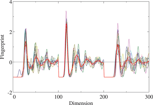
Å were set according to the arguments given in Sect. 2.1. Actually, clear dips are commonly seen just beyond the first NN O-Al pair shell in the
-fingerprint of all the systems as shown in . Two amorphous structures are quite similar each other in the
-fingerprint while some recognizable differences can be seen in the O-Al and Al-Al pair regions beyond the NN distance. They are also similar to the crystalline polymorphs within the first NN shell of the O-O, O-Al, and Al-Al pairs and turn to be remarkably broadened beyond. Such features were found and discussed in detail by Momida et al. [Citation43]. Distances are calculated using Euclidean and Cosine distance schemes up to the radius cutoff of
Å and
Å and the eigenvalues and eigenvectors of the double-centered squared distance matrix are computed to get the structure coordinates as described in Sects. 2.2 and 2.3.
Figure 2. F-Fingerprint of all the AlO
systems listed in except for the 2D film model. Radius cutoff
Å is assumed and the fingerprint of dimensions between 0 and 100, 101 and 200, and 201 and 300 corresponds to O-O, O-Al, and Al-Al pairs, respectively. Line colors follow color scheme in Table 1 for distinguishing different structures.
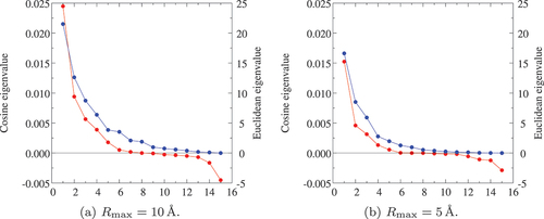
In , calculated eigenvalues are drawn for two radial cutoffs Å and
Å with Euclidean and Cosine distances (EquationEquation (9)
(9)
(9) and (Equation6
(6)
(6) ), respectively). Typical lattice constants of the systems we consider are up to about 10 Å and the cutoff
Å should naívely be appropriate as the first choice. To see effects of the assumed cutoff on structure analyses, a study with
Å is also tested. Looking at the Euclidean-distance eigenvalues in ,
Å gives relatively larger eigenvalues than
Å. However, the proportion with
Å (
and
) is not so different from that with
Å (
and
). In the case of Cosine distance, the behavior of eigenvalues closely resembles the Euclidean one but information estimation only by the proportion is a bit ambiguous due to the existence of negative eigenvalues. It should be done by testing the precision in models constructed with the obtained PCs as descriptors, as we shall see below.
Figure 3. Eigenvalues calculated from the fingerprint of AlO
polymorphs using (a)
Å and (b)
Å with Euclidean (blue) and cosine (red) distances.
shows coordinate map of all the AlO
structures on five PCs (
through
as the first five components of
given in EquationEquation (12)
(12)
(12) ) with different radial cutoff and type of distance. The distribution of the structures in the maps with different cutoff and type of distance is generally quite similar. Most typically, the three lowest-energy structures (SG:
(black),
(maroon), and
(blue)) form line-shaped clustering on the
-
dimension. Relatively low-energy structures up to about 100 meV/atom surround the lowest-energy cluster forming a basin except for
structure (pink) that is the most stable for In
O
, far outside along the PC
. Two amorphous structures are located near the edge of the basin close to the highest-energy structure (
). The
structure is situated close to the lowest-energy one (
) along
through
axes and found to be distinguishable along
or
. It is also interesting that the stable structures of Ga
O
(
: maroon) and In
O
(
: pink) reveal relatively low energy while their positions in the map are far especially along
. Since the PC
dominantly contains information of the first NN O-Al pairs as shown below, the coordination number and the length variation in the NN O-Al bonds by local symmetry seem to affect the distance (dissimilarity) in the structure map.
Figure 4. Map of AlO
structures with the five principal components (PCs) with (a) Euclidean-distance
Å, (b) cosine-distance
Å, (c) Euclidean-distance
Å, and (d) cosine-distance
Å. Dot colors follow color scheme listed in . Square dots in each figure denote the three lowest energy structures (SG:
(black),
(maroon), and
(blue)), and small and large red dots express amorphous model structures (SG:
) by the materials project [Citation11] and momida [Citation43], respectively.
![Figure 4. Map of Al 2O 3 structures with the five principal components (PCs) with (a) Euclidean-distance Rmax=10 Å, (b) cosine-distance Rmax=10 Å, (c) Euclidean-distance Rmax=5 Å, and (d) cosine-distance Rmax=5 Å. Dot colors follow color scheme listed in Table 1. Square dots in each figure denote the three lowest energy structures (SG: R3ˉc (black), C2/m (maroon), and Pna21 (blue)), and small and large red dots express amorphous model structures (SG: P1) by the materials project [Citation11] and momida [Citation43], respectively.](/cms/asset/95d8b270-b3fc-4290-b32a-f048af2e6be4/tstm_a_2355860_f0004_oc.jpg)
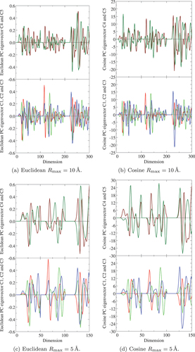
To investigate the information and its meaning immanent in each PC and the corresponding coordinates, the eigenvector of the obtained PCs is calculated using EquationEquation (17)(17)
(17) and plotted in . By searching the largest amplitude of each PC eigenvector in , one can find which radial part of the
-fingerprint, namely RDF gives the most important contribution to the PC. The fist PC
has the largest amplitude at the first NN position of the O-Al pair, irrespective to the choice of the radial cutoff and type of distance. The second PC
shows the largest contribution from the second and third NNs of O-Al pair and almost equally the first NN of O-O pair. From these findings, it seems that the characteristics in the energy landscape seen in may be quantitatively explained by the O-Al and O-O neighboring environmental features. However, the PCs beyond
and
are also significantly important to reproduce the energy more precisely, as shown below. In this context, the largest amplitudes for
,
, and
can be seen for the Al-Al RDF.
Figure 5. Eigenvector of the five principal components (PCs) with (a) Euclidean-distance Å, (b) cosine-distance
Å, (c) Euclidean-distance
Å, and (d) cosine-distance
Å, calculated by using EquationEquation (17)
(17)
(17) in Al
O
polymorphs. Red, lime, blue, maroon, and green lines denote
,
,
,
, and
PC, respectively. Horizontal axis denotes the dimension of the original fingerprint space (see ). In (a) and (b), the dimensions between 1 and 100, 101 and 200, and 201 and 300 express the O-O, O-Al, and Al-Al pair radius, respectively, and in (c) and (d), the dimensions between 1 and 50, 51 and 100, and 1001 and 150 do the O-O, O-Al, and Al-Al pair radius, respectively.
A sparse modeling technique is useful to search the important descriptors among a given set of ones. In the present study, we prepared 21 descriptors of the zero-th (constant term) through second orders of the obtained five PCs (—
), and detected and removed their collinearity and multi-collinearity (linear dependence), and then used exhaustive search or genetic algorithm in linear regression analysis. The best set of the descriptors for a fixed number of descriptors is selected by the leave-one-out (LOO) scheme, a kind of cross validation techniques [Citation47]. Results of the regression analysis for the total energy using the PCs as the descriptors are shown in .
is the coefficient of determination widely used for expressing the fitting performance [Citation48],
is the coefficient of determination for the prediction residual sum of squares (often called PRESS) showing a measure of generalization capability [Citation49] and RMSE denotes the root mean square error in the regression. The explicit equations of these quantities are given and discussed in our previous study [Citation47]. At glance, good modeling is achieved as the number of descriptors is increased in all the cases and any over-fitting behaviors those are often observed in
are not seen, possibly because of the use of orthogonal PCs as the descriptors. Although the products of the PCs used may not necessarily be orthogonal to the others, any collinearity or multi-collinearity tendency has not been detected up to the second order of the PCs. As a more rigorous test for investigating any existing over-fitting, a double cross-validation technique is adopted. Here, one sample data are completely hidden during the modeling and then the best model trained by the LOO method with the remaining data is tested for checking the generalization capability using the hold-out data. Double cross-validation results for the total-energy model constructed from the Euclidean distance with
Å are shown in . As the number of descriptors is increased, the standard deviation for the prediction error of the hold-out data shows first a decline, then minimum (
eV) at the number of descriptors of eight and an ascent beyond, indicating the over-fitting behavior with large numbers of descriptors. The explicit model form with the number of descriptors of eight is
Figure 6. Regression analysis of the total energy with descriptors up to the second order of the five PCs in AlO
polymorph structures. (a) Euclidean-distance
Å, (b) cosine-distance
Å, (c) Euclidean-distance
Å, and (d) cosine-distance
Å. Blue, red, and green dots and lines denote the coefficient of determination (
), its leave-one-out coefficient (
), and root mean square error (RMSE), respectively.
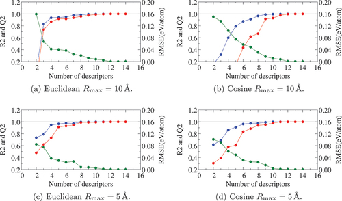
Figure 7. Double cross-validation test of the total-energy regression model constructed with the descriptors from the Euclidean distance and Å in Al
O
polymorph structures. Dot colors follow color scheme listed in . Red open circle denotes one of the amorphous structure (mp -1,245,063). The model of the number of descriptors of eight shows the smallest standard deviation (
0.1 eV).
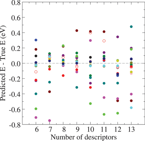
All of the PCs, through
are selected in the model. Detailed energy landscape is actually very complicated than just looking at the map (). The double cross-validation test tells that the line-shaped dip seen in the
-
map is rather shallow in the basin landscape and not well precisely reflected in the regression model, though higher-energy structures than 0.1 eV including the amorphous models are well distinguished in the energy model.
It is found, in the same way as the total-energy regression, that the energy-gap data given in can be also modeled with the same structural descriptors, namely through
and their products up to the second order plus the constant term, at the similar level of precision.
3.2. Site preference in La(Fe,Si)13
As a second application of the proposed workflow, we consider the classification of alloy-type configurations for analyzing the site preference of doped Si atoms in LaFeSi
. This compound is well known as a magnetocaloric materials in applications for magnetic refrigeration [Citation50]. The crystal structure of LaFe
Si
is of cubic NaZn
type (SG:
) for
[Citation51–53] and drawn in with VESTA [Citation9]. There are two kinds of crystallographic sites for Fe: Fe1 (
Wyckoff position) and Fe2 (
), and doped Si atoms share the
site with Fe2. Configurations of Fe2 and Si are discussed as ‘coloring problem’ [Citation53]. Let us consider below a primitive cell La
Fe
Si
(
) of the system with fixed experimental lattice constants and atomic positions taken from the database COD-1528546 [Citation7].
Figure 8. Crystal structure of LaFe
Si
. Green, orange, and brown balls denote La, Fe1 and Fe2 atomic sites, respectively. Partial occupation of Si at the Fe2 sites is depicted with blue. The drawing is made with VESTA [Citation9].
![Figure 8. Crystal structure of La 2Fe 26−ySi y. Green, orange, and brown balls denote La, Fe1 and Fe2 atomic sites, respectively. Partial occupation of Si at the Fe2 sites is depicted with blue. The drawing is made with VESTA [Citation9].](/cms/asset/c692dc0d-6af6-4472-9e52-9b01d2617856/tstm_a_2355860_f0008_oc.jpg)
Looking at the local coordinates around Fe, the Fe1 () site is coordinated by 12 Fe2 at the distance of 2.46 Å, which is the similar NN distance to that of pure BCC Fe. This means that the Fe1 site is closely packed with a high coordination number. Around the Fe2 (
) site, on the other hand, there are two Fe2 at 2.45 Å, one Fe1 at 2.46 Å, and seven Fe2 in a range of 2.50–2.69 Å, showing less densely packed than Fe1. Although the atomic radius of Si is 1.17 Å slightly smaller than that of Fe of 1.24 Å [Citation54], the site preference of Si at the Fe sites is not so easily understandable at first glance.
In the case of LaFe
Si
, there are only two possible inequivalent configurations with one Si atom either at the
or
site (Case 1). It turns to be a bit complicated situation in La
Fe
Si
. There is one configuration with two Si atoms fully occupying at the
site (Case 2–1). If two Si atoms are placed one by one at the
and
sites (Case 2–2), total number of possible configurations is 48 (=
C
C
). By analyzing the structural similarity as described above, it is reduced to two crystallographically inequivalent structures. If two Si atoms are accommodated at the
sites (Case 2–3), there are 276 (=
C
) possible configurations. And then, one can easily obtain 12 crystallographically inequivalent structures by the distance diagnosis. Similarly, in La
Fe
Si
there are one crystallographically inequivalent structure out of 24 possible configurations for two Si at
and one Si at
(Case 3–1), 17 crystallographically inequivalent structures out of 552 (=
C
C
) configurations for one Si at
and two Si at
(Case 3–2), and 50 inequivalent structures out of 2024 (=
C
) configurations for three Si at
(Case 3–3). In all the cases of this sub-section, the crystallographically inequivalent structures correspond to the distinct pair-wise fingerprints.
Heats of formation per atom are evaluated from total energies by first-principles DFT calculations with the FLAPW method for the configuration () in La
Fe
Si
(
) and most-stable elemental crystal systems, La (
), ferromagnetic Fe (
), and Si (
) as
and plotted in together with spin magnetic moments per Fe atom. To see the configurational energy for a given , the heats of formation relative to the lowest energy value at
that correspond to the configurational energy defined as
Figure 9. Heats of formation in eV/atom (EquationEquation (22)
(22)
(22) ) and
in meV/atom (EquationEquation (23)
(23)
(23) ), and spin magnetic moments in
per Fe atom calculated for La
Fe
Si
. Red dots, green dots, and blue circles denote values for the configurations with Si occupying at only
, at
and
, and at only
, respectively. Black dots indicate the corresponding values for La
Fe
.
![Figure 9. Heats of formation H in eV/atom (EquationEquation (22)(22) H(y;i)=128{E[La2Fe26−ySiy;i]−2E[La] −(26−y)E[Fe]−yE[Si]}(22) ) and ΔH in meV/atom (EquationEquation (23)(23) ΔH(y;i)=H(y;i)−minjH(y;j)(23) ), and spin magnetic moments in μB per Fe atom calculated for La 2Fe 26−ySi y. Red dots, green dots, and blue circles denote values for the configurations with Si occupying at only 8b, at 8b and 96i, and at only 96i, respectively. Black dots indicate the corresponding values for La 2Fe 26(y=0).](/cms/asset/4d6d57dc-1c0b-48d0-b677-6af56fa267a7/tstm_a_2355860_f0009_oc.jpg)
are also drawn. The calculated heat of formation for non-doped LaFe
is
meV/atom, indicating unstable to the constituent elemental systems consistent with no intermetallic-compound phase in the experimental phase diagram [Citation55]. As the composition of Si
is increased in La
Fe
Si
, the systems show a nearly linear stability to
with negligibly small configurational variation at the energy scale of eV/atom within the same
. Minor in magnitude but interesting behaviors in the configurational energy
at the 10 meV/atom energy scale are discussed below. Calculated spin magnetic moment per Fe atom is monotonically decreased as
is increased, leading to reduction in total magnetization per cell more than that simply by the decrease in the number of Fe atoms. Interestingly, the spin magnetic moment shows certain dependence on the configuration within the same Si concentration possibly due to differences in the local hybridization between Fe and Si atoms.
The configurational energy at in tells that Si prefers to be accommodated at the Fe2 (
) site by 11 meV/atom compared with the Fe1 (
) site, being consistent with the experimental data (COD-1528546) [Citation7]. Since the multiplicity of the Fe2 site (24) is significantly larger than that of the Fe1 site (2), the entropic effect must additionally contribute to the site-preference of Si at the Fe2 site. A rough estimation of the difference in the configurational entropy gives
meV/K-cell, implying the same order contribution as the energy difference to the stability at temperatures of several hundreds K. By inspecting the configurational energy
more carefully in , clustering features can be seen for Si occupying at the
sites (most remarkably in blue circles of
and
). Since the clustering features are possibly related to the origin of the configurational stability, structure map for all the inequivalent configurations may be useful for understanding it with the benefit of the prescriptions explained in Sec. 2.
shows the -fingerprints and eigenvector of three PCs on the Si-Si and Fe-Si dimensions of La
Fe
Si
(Case 2–3). The
-fingerprints on the Fe-Si dimension show very minor differences compared with those on the Si-Si one and the other
-fingerprints are much weakly distinguishable (not included in the figure). Among the 12 inequivalent configurations, four structures have two Si atoms located at the NN
sites and are in relatively high energy (+7.9 — +20.7 meV/atom) above the lowest energy in the configurational energies
at
in . The rest of the configurations have no NN Si pair and their energies are below +2.6 meV/atom. The PC
of the structure map of the Euclidean distance in clearly distinguish the four high-energy configurations and the rest of eight ones. The proportion of
is
. The eigenvector of
shown in actually has the largest amplitude around the Si-Si NN distance. The PCs
and
have the largest amplitude of the eigenvectors around approximately 4 Å and 6 Å, respectively, and are related to the different stability within the
-clustering structures. The three structures (blue, cyan, and teal) with the NN Si-Si pair are quite similar in the map up to the PC
and the PCs beyond must determine the minor energy difference. It is concluded that the interaction between the Si atoms are repulsive in La
Fe
Si
and they may tend to be distributed apart.
Figure 10. (a) -fingerprints and (b) Euclidean eigenvectors of three principal components of Si-Si (0–80) and Fe-Si (80–160) dimensions of La
Fe
Si
(Case 2–3). Line colors used for the
-fingerprints in (a) correspond to those of dots in . Red, lime, and blue lines in (b) denote the eigenvectors of
,
, and
, respectively.
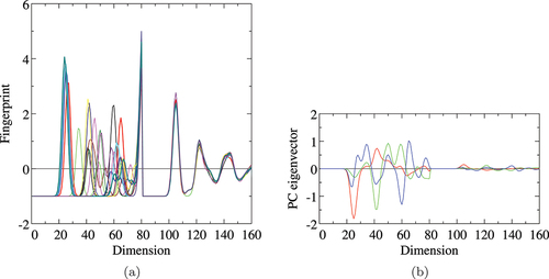
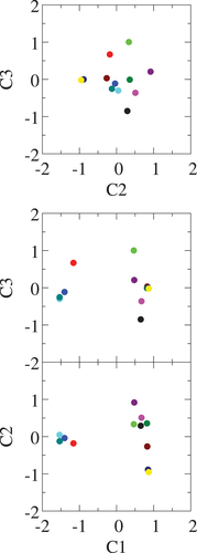
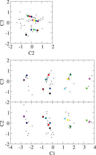
Figure 11. Structure map of LaFe
Si
(case 2–3) obtained by dimension reduction of the Euclidean distance. Dot colors denote the different configurations corresponding to the
-fingerprint shown in ).
Some selected -fingerprints showing distinctive behavior and eigenvectors of three PCs on the Si-Si and Fe-Si dimensions of La
Fe
Si
(Case 3–3) are drawn in . The corresponding structure map of the Euclidean distance with
is shown in , resulting in the proportion
. The eigenvectors of the three PCs contain the structure information around the essentially same regions of the feature vector dimension as the previous case of La
Fe
Si
(Case 2–3). In this case, there are four kinds of the
-fingerprint peak height at the NN Si-Si distance. The structures (magenta and lime) possessing the highest RDF at the NN distance has Si triangular trimers, forming a clustering with two more structures (small black) in the structure map. The structures (cyan, yellow, and green) with the second highest RDF have V-shape Si trimers, those (maroon, teal, red, blue, and black) with the third highest RDF do Si dimers, and those (purple and navy) have no NN Si pair. These locally distinct Si structures are clearly classified in the structure map along the PC
, also being in accordance with the general repulsive behavior between the Si atoms in the configurational stability in La(Fe,Si)
.
Figure 12. (a) Selected -fingerprints and (b) eigenvectors of three principal components of Si-Si (0–80) and Fe-Si (80–160) dimensions of La
Fe
Si
(case 3–3). Red, lime, and blue lines in (b) denote the eigenvectors of
,
, and
, respectively.
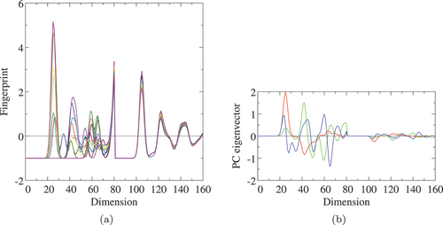
Figure 13. Structure map of LaFe
Si
(case 3–3) obtained by dimension reduction of the Euclidean distance. Dot colors denote the different configurations corresponding to the
-fingerprint shown in ), where the
-fingerprints of the small black dots here are not included.
4. Summary
The three-step procedure to draw crystal structure map for a given set of materials systems with the same composition is proposed and demonstrated to classify the structure in a low-dimensional space and to model the materials properties. Combined with the scheme for counting all the possible combinations for alloy systems within supercell models, configurational energy preference can be discussed with the multiplicity of each configuration as the entropic effect. Further applications of the present methods with first-principles DFT calculations and machine-learning analysis are highly expected. In addition, regarding future prospects the present procedure may be applicable to any vector-type information such as spectral and image data for a given set of related materials systems. Map obtained in a low-dimensional space classifies the existing materials systems in terms of the reduced features and may possibly assist to explore desired candidate systems by using the projection and inverse-projection techniques as shown in EquationEquation (19)(19)
(19) and (Equation20
(20)
(20) ).
Statement of novelty
Crystal structure map constructed from the feature of structures by a dimension-reduction technique for classification and modeling for a group of related materials such as polymorphs, alloys, and doped systems.
Acknowledgements
The author would like to thank Hiroyoshi Momida for providing the structure data of the amorphous AlO
model, Yukihiro Makino, Tetsuya Fukushima, and Kazunori Sato for invaluable discussion in the study of La(Fe,Si)
, and Hitoshi Fujii, Tomoki Yamashita, Hiori Kino, and Takashi Miyake for suggestive comments on data-science techniques.
Disclosure statement
The author declares no known competing financial interests.
Data availability statement
The raw data required to reproduce these findings are available by making an e-mail request to the corresponding author.
Additional information
Funding
References
- Jose R, Ramakrishna S. Materials 4.0: materials big data enabled materials discovery. Appl Mater Today. 2018;10:127–16. doi: 10.1016/j.apmt.2017.12.015
- Day GM, Cooper AI. Energy–structure–function maps: cartography for materials discovery. Adv Mater. 2018;30(37):1704944. doi: 10.1002/adma.201704944
- Born M, Oppenheimer R. Zur Quantentheorie der Molekeln. Ann Phys. 1927;389(20):457–484. doi: 10.1002/andp.19273892002
- CIF Dictionary. Available from: https://www.iucr.org/resources/cif/dictionaries/
- International Union of Crystallography (IUCr). Available from: https://www.iucr.org/
- The Inorganic Crystal Structure Database (ICSD). Available from: https://icsd.fiz-karlsruhe.de/
- Crystallography Open Database (COD). Available from: http://www.crystallography.net/cod/
- AtomWork. Available from: https://crystdb.nims.go.jp/
- Momma K, Izumi F. VESTA: a three-dimensional visualization system for electronic and structural analysis. J Appl Crystallogr. 2008;41:653–658. Available from: https://jp-minerals.org/vesta/en/
- CrystalMaker Software. Available from: https://crystalmaker.com/
- The Materials Project. Available from: https://materialsproject.org/
- NOMAD Center of Excellence. Available from: https://nomad-coe.eu/
- The Open Quantum Materials Database (OQMD). Available from: http://oqmd.org/
- The AFLOW standard encyclopedia of crystallographic prototypes. Available from: http://aflowlib.org/prototype-encyclopedia/
- Stokes HT, Hatch DM. FINDSYM: program for identifying the space-group symmetry of a crystal. J Appl Cryst. 2005;38(1):237–238. doi: 10.1107/S0021889804031528
- Stokes HT, Hatch DM, Campbell BJ. FINDSYM, ISOTROPY software suite. Available from: https://iso.byu.edu/
- Connolly JWD, Williams AR. Density-functional theory applied to phase transformations in transition-metal alloys. Phys Rev B. 1983;27(8):5169–5172. doi: 10.1103/PhysRevB.27.5169
- Oganov AR, Valle M. How to quantify energy landscapes of solids. J Chem Phys. 2009;130(10):104504. doi: 10.1063/1.3079326
- Yamashita T, Sato N, Kino H, et al. Crystal structure prediction accelerated by Bayesian optimization. Phys Rev Mater. 2018;2(1):013803. doi: 10.1103/PhysRevMaterials.2.013803
- Sato N, Yamashita T, Oguchi T, et al. Adjusting the descriptor for a crystal structure search using bayesian optimization. Phys Rev Mater. 2020;4(3):033801. doi: 10.1103/PhysRevMaterials.4.033801
- Yamashita T, Kanehira S, Sato N, et al. CrySPY: a crystal structure prediction tool accelerated by machine learning. Sci Technol Adv Mater. 2021;1(1):87–97. doi: 10.1080/27660400.2021.1943171
- Bartók AP, Kondor R, Csányi G. On representing chemical environments. Phys Rev B. 2013;87(18):184115. doi: 10.1103/PhysRevB.87.184115
- Zimmermann NER, Jain A. Local structure order parameters and site fingerprints for quantification of coordination environment and crystal structure similarity. RSC Adv. 2020;10(10):6063–6081. doi: 10.1039/c9ra07755c
- Torgerson WS. Multidimensional scaling: I. Theory and method. Psychometrika. 1952;17(4):401–419. doi: 10.1007/BF02288916
- Borg I, Groenen P. Modern multidimensional scaling, springer series in statistics. NY: Springer; 1997. Chap. 12, p. 261–267. doi: 10.1007/978-1-4757-2711-1_12
- Cox TF, Cox MAA. Multidimensional scaling. 2nd ed. Boca Raton (FL): Chapman & Hall/CRC; 2001.
- Sibson R. Studies in the robustness of multidimensional scaling: perturbational analysis of classical scaling. J R Statist Soc B. 1979;41(2):217–229. Available from: https://www.jstor.org/stable/2985036
- Cox MAA, Cox TF. Handbook of data visualization. Chen C, Härdle W Unwin A, editors. Vol. Chap. III.3. Berlin: Springer-Verlag; 2008. p. 315–347. doi: 10.1007/978-3-540-33037-0_14
- Bishop CM. Pattern recognition and machine learning. NY: Springer-Verlag; 2006.
- Soven P. Coherent-potential model of substitutional disordered alloys. Phys Rev. 1967;156(3):809–813. doi: 10.1103/PhysRev.156.809
- Ehrenreich H, Schwartz LM, Ehrenreich H, Seitz F, Turnbull D, editors. Solid state physics. Vol. 31. NY: Academic Press; 1976. p. 149.
- Shiba H. A reformulation of the coherent potential approximation and its applications. Prog Theor Phys. 1971;46(1):77–94. doi: 10.1143/PTP.46.77
- Korringa J. On the calculation of the energy of a Bloch wave in a metal. Physica. 1947;13(6–7):392–400. doi: 10.1016/0031-8914(47)90013-X
- Kohn W, Rostoker N. Solution of the schrödinger equation in periodic lattices with an application to metallic lithium. Phys Rev. 1954;94(5):1111–1120. doi: 10.1103/PhysRev.94.1111
- Zunger A, Wei S-H, Ferreira LG, et al. Special quasirandom structures. Phys Rev Lett. 1990;65(3):353–356. doi: 10.1103/PhysRevLett.65.353
- Wei S-H, Ferreira LG, Bernard JE, et al. Electronic properties of random alloys: special quasirandom structures. Phys Rev B. 1990;42(15):9622–9649. doi: 10.1103/PhysRevB.42.9622
- Wimmer E, Krakauer H, Weinert M, et al. Full-potential self-consistent linearized-augmented-plane-wave method for calculating the electronic structure of molecules and surfaces: O2 molecule. Phys Rev B. 1981;24(2):864–875. doi: 10.1103/PhysRevB.24.864
- Weinert M, Wimmer E, Freeman AJ. Total-energy all-electron density functional method for bulk solids and surfaces. Phys Rev B. 1982;26(8):4571–4578. doi: 10.1103/PhysRevB.26.4571
- Soler JM, Williams AR. Augmented-plane-wave forces. Phys Rev B. 1990;42(15):9728–9731. doi: 10.1103/PhysRevB.42.9728
- Oguchi T, Terakura K, Akai H, editors. Inter-atomic potentials and structural stability. Berlin: Springer-Verlag; 1993. p. 33–41.
- Perdew JP, Burke K, Ernzerhof M. Generalized gradient approximation made simple. Phys Rev Lett. 1996;77(18):3865–3868. doi: 10.1103/PhysRevLett.77.3865
- Blöchl PE, Jepsen O, Andersen OK. Improved tetrahedron method for Brillouin-zone integrations. Phys Rev B. 1994;49(23):16223–16233. doi: 10.1103/PhysRevB.49.16223
- Momida H, Hamada T, Takagi Y, et al. Theoretical study on dielectric response of amorphous alumina. Phys Rev B. 2006;73(5):054108. doi: 10.1103/PhysRevB.73.054108
- Zhu C, Xue J. Structure and properties relationships of β-Al2O3 electrolyte materials. J Alloys Compd. 2012;517:182–185. doi: 10.1016/j.jallcom.2011.12.080
- Samain L, Jaworski Edén AM, Ladd DM, et al. Structural analysis of highly porous γ-Al2O3. J Solid State Chem. 2014;217:1–8. doi: 10.1016/j.jssc.2014.05.004
- Rudolph M, Motylenko M, Rafaja D. Structure model of γ-Al2O3 based on planar defects. IucrJ. 2019;6(1):116–127. doi: 10.1107/S2052252518015786
- Kanda Y, Fujii H, Oguchi T. Sparse modeling of chemical bonding in binary compounds. Sci Tech Adv Mater. 2019;20(1):1178–1188. doi: 10.1080/14686996.2019.1697858
- Kvalseth TO. Cautionary note about R2. Am Stat. 1985;39(4):279–285. doi: 10.1080/00031305.1985.10479448
- Schüürmann G, Ebert R-U, Chen J, et al. External validation and prediction employing the predictive squared correlation coefficient — test set activity mean vs training set activity mean. J Chem Inf Model. 2008;48(11):2140–2145. doi: 10.1021/ci800253u
- Fujita A, Fujieda S, Hasegawa Y, Fukamichi K. Itinerant-electron metamagnetic transition and large magnetocaloric effects in La(FexSi1-x)13 compounds and their hydrides. Phys Rev B. 2003;67(10):104416. doi: 10.1103/PhysRevB.67.104416
- Krypyakevych PI, Zarenchnyuk OS, Gladyshevskii EI, et al. Ternäre verbindungen vom NaZn13-Typ. Anorg Allg Chem. 1968;358(1–2):90–96. doi: 10.1002/zaac.19683580110
- Tang W, Liang J, Guanghui R, et al. Study of AC susceptibility on the LaFe13–xSix system. Phys Status Solidi A. 1994;141(1):217–222. doi: 10.1002/pssa.2211410121
- Han M-K, Miller GJ. An application of the “coloring problem”: structure−composition−bonding relationships in the magnetocaloric materials LaFe13-xSix. Inorg Chem. 2008;47(2):515–528. doi: 10.1021/ic701311b
- Emsley J. The elements. 3rd ed. Oxford: Clarendon Press; 1998.
- Gschneidner KA, Massalski TB., editor. Binary alloy phase diagrams. II Ed. Vol. 2. OH: ASM International; 1990. p. 1718–1719.