Biometric voice recognition system in the context of multiple languages: using traditional means of identification of individuals in Nigeria languages and English language

Abstract.

Voice biometrics is challenging in many aspects, ranging from voice data acquisition through processing down to the matching module. Some of the challenges of an automatic voice biometric are background noises, mimicry, voice playback, and so on. This research work emphasizes identifying a person in the context of varying languages. Mel-Frequency Cepstral Coefficient (MFCC), Gammatonne Cepstral Coefficient (GTCC), the Pitch, and the iVector are feature extractor techniques that are amazing for differentiating individuals. In this research work, a new feature extractor derived from Pitch, GTCC, and MFCC is proposed. A novel AfroVoices database of 94 subjects was collected with ten (10) voiceprints of Nigerian localities: five (5) spoken in English and five (5) in vernacular, resulting in a total of 940 voiceprints. The experiment was performed on three datasets AfroVoices, UNN_BVC, and LibriSpeech voice datasets, which were done in the MATLAB environment. The experiment was performed using the traditional approach of recognizing individuals using the biometric system. Experimenting reveals that varying languages do not affect voice biometric performance. It also reveals that the presence of noise affected the performance of the system, as the clean utterances performed relatively better.

Keywords:

• Gammatone cepstral coefficient
• Mel frequency cepstral coefficient
• feature extractors
• vernacular
• pre-recorded
• voice-biometric

1. Introduction

The requirement for biometric authentication for humans in the real world has brought about an ongoing research topic on the use of biometric technologies (Hansen and Hasan 2015). Vocal communication is very important, as it is one of the means of effective and efficient communication exhibited by the human race. There are means through which clear communication can be carried out easily. Information about the state of a speaker’s emotions can be perceived from a voice (Tovarek et al. 2018). However, listening to conversations can not only predict how many people have spoken in that hall but also indicate who owns the phone. Voiceprints, on the other hand, represent a person’s accent, intonation, rhythm, and a combination of physical factors that provide information about the size and shape of a person’s nasal passages, the length, and diameter of the vocal tract. Information filtered from the audio signal, such as the vocal cords, can predict the speaker’s gender, ethnicity, age, and possibly height (Latinus and Belin 2011). The first dominant application of biometric identification can be traced back to World War II. At this time, U.S. soldiers used machines called spectrographs to intercept voice transmissions and track down their enemies. Spectrographs were primitive and flawed until 1976 when Texas Instruments created the first modernized voice biometric engine with the ability to more accurately register and determine the end user’s voiceprint (Maltoni et al. 2009). Voice has long been used as a means of recognizing people, but as a biometric modality, it is not a new way of identifying people. As recorded in the Christian scriptures, speaker recognition was primitively demonstrated in the account of Esau and his brother Jacob. There, Jacob conspired with his mother to deceive his father, Isaac, and evade the blessing his father was going to give his first son, Esau. So Jacob clothed himself in animal skins to create a hairy texture like Esau’s. When Jacob appeared, Isaac was skeptical, and unconvinced and wanted to hear the voice of his son Esau before blessing him. Hold on, “The voice is the voice of Jacob, and the hand is the hand of Esau” (Genesis 27:22 NIV). Jacob played a practical joke on his father (biometric theft) to gain access to a blessing that was not meant for him. Isaac used his two biometric modalities to try to identify his son, his voice, and his body hair, but his voice failed. The dying father had no choice but to advise him to bless the wrong person (false acceptance). Jacob tricked his father by presenting a hairy skin forged from animal fur. Probably because he was dying, it is clear that his accuracy rate was rather low. This is a prime example of the benefits of using multiple biometric modalities to identify and verify an individual. Single-modality systems are more likely to be circumvented or manipulated than multimodality biometric systems (Ajimah et al. 2017).

1.1. Problem statement

Voice biometrics is the most difficult biometric method to use to identify people. This is because the human voice is affected by many factors, such as age, illness, ascension, mood, vocal cord length, vocal cord radius, tooth arrangement, and weight. Body weight or height. Meanwhile, other biometric modalities like the fingerprint, face, palm print, iris, hand geometry, and the most efficient are multimodal systems (fusion of several biometric modalities) are not affected by illness, age, or mood, thus, other forms of biometrics can stand the test of time. All these factors give rise to challenges in speaker recognition systems. There are imitation problems, where people try to talk like everyone else and gain access to a facility they are not allowed to enter. Some problems with speaker recognition systems are related to administrators preventing real people from accessing the installation or adding fake users. Furthermore, there are situations where the voice is recorded in a quiet environment and some come from a noisy background, which greatly affects the performance of the system. Mel Frequency Cepstral Coefficient (MFCC) and Gammatone Central Factor (GTCC) are household names in speech feature extractors, but as is the challenge of voice biometrics, based on recognition speed, personal recognition accuracy, and tolerance. In noisy environments, it seems like a lot of work needs to be done to improve the extraction of vocal characteristics. In the literature, it has been shown that very few researchers have tested on many different languages, especially local African languages, so having online voice repositories of local languages in Africa’s monopoly is quite rare. As such, most of the online repositories are in the primary languages of Europeans, Americans, and some Asian countries. In this work, a system was developed using the traditional approach which entails assemblies of voice input, feature extractor, feature storage, matcher (for matching of the features during the query stage), and the decision maker (which takes decisions based on the set thresholds).

1.2. Aim and objectives of the research

This research work is aimed at developing a voice biometric system for recognizing individuals in the context of varying languages as well as a new twist in feature extraction using some mathematical models. The work will involve collating an English and vernacular voice database from native Nigerians of various ethnicities. The following are the goals for realizing the aim of the research:

1. To extract robust feature descriptors from voice suitable to characterize each person’s voice.

2. To develop a robust traditional-based speaker recognition system

3. To evaluate the performance of proposed models on the database of English and vernacular languages

4. To evaluate the proposed feature extraction model on public voice databases and compare results with those of existing approaches.

1.3. Scope of study

This research work focuses on a biometric speaker recognition system for loud and clear voice data. The relevance of working on clean and noisy data is to ensure that our proposed model can perform optimally in all environments since we cannot always be in a quiet environment. A type of speech feature extraction generated from mathematical equations from Gaussian, spherical, and electric field potentials. This new feature class is compared in terms of performance with existing traditional speech feature extraction techniques such as MFCC, GTCC, and a combination of delta, the change of the MFCC or GTCC extracted feature and their acceleration which is represented as deltaDelta, is the change of the MFCC or GTCC delta feature. Different works have been done on voices, and different techniques used in speech feature extraction were considered in this research work. Instructions and books have been researched to give a clearer picture of the subject. The database of short speech phrases was collected using the Audacity application installed on the HP Windows operating system, a quad-core Intel processor (2.16 GHz), and its built-in microphone for voice collection. This new database formed 10 voices (5 English voices and 5 dialect voices) out of 94 subjects. Total impressions are 940 (i.e., 470 in English and 470 in the mother tongue). In addition, a new speech feature extraction system has been modelled using several mathematical equations. Testing was performed in the MATLAB environment using the Audio Toolkit. The experiment was repeated on two other existing databases (UNN_BVC).

1.4. Motivations

Voice recognition is a form of personal recognition that helps recognize individuals by their voice, regardless of what or how it is been said. This type of engineering technology is applied to most automated systems due to its transparency and accessibility. Voice is a special type of biometric because it involves physiological and behavioral characteristics in identification. This aspect of voice gives rise to its complex nature and was the challenge that interested me in undertaking this study to recognize people in noisy and quiet environments. In popular voice feature extraction like the MFCC and the GTCC the MFCC finds it difficult to identify the individual with varying pitch, the GTCC is not affected by the pitch but vulnerable to noise. In this research, we have proposed a hybrid model of MFCC and GTCC to address some of the shortcomings of the aforementioned feature extraction techniques.

1.5. Significance

This paper will contribute to the biometrics research community and to novices aspiring to join the biometric research cluster. Today, biometrics can be linked to everything we do in our daily lives, so voice biometrics is not an exception. Almost every field of technology finds relevance in this area of study. This work provides English and vernacular speech datasets for researchers in the field of speaker recognition systems and other aspects of signal processing.

1.6. Proposed method

This paper placed more emphasis on the recognition of individual by their voices. Despite facing some challenges faced by speaker recognition features, the research has developed a new feature extraction modelled from the Gaussian equation, spherical equation, and the potential equation that comes from the pitch, MFCC, and GTCC to identify individuals. It is clear that the performance of the biometric system is enhanced by a combination of multiple biometric features or types this study focuses on studying the performance of the voice biometric system on different datasets, and variant features are extracted to recognize accuracy in various performance index (Ortega et al. 2010).

Experiments were performed on three datasets, one of which was a new dataset, collected locally in Nigeria. Data collection was performed with Audacity software and the integrated microphone HP 250. Traditional experiments were performed in the MATLAB environment. The other databases for this test are the LibriSpeech and UNN_BVC databases. A new voice feature extraction type derived from GTCC and MFCC and modeled in the combination of Gaussian, spherical, and electric field mathematical equations. The performance of this feature model is compared with existing feature extraction techniques such as GTCC and MFCC, as well as their velocity and acceleration.

In Section 2, we looked at the overview of voice authentication and verification systems and their relevance in our everyday lives. We also looked at some motivation behind Voice feature extraction (though more emphasis was on Mel Frequency Cepstral Coefficient, MFCC and Gammatone Cepstral Coefficient, GTCC), furthermore, we reviewed related articles from several authors. In Section 3, we descriptively outlined the materials and methods used in this research. The database representation was discussed as well. Furthermore, we spelt out the performance metric used to ascertain the precision of the developed model. In Section 4, we reported the results of the experiments performed on the Afrovoices, UNN_BVC, and LibriSpeech databases and also compared their performances relative to the extracted features. In Section 5, we concluded and recommended trends for future work.

2. Voice biometrics and the systems

Voice biometrics is a technology that uses the nature of how humans produce sound, also known as voice biometrics, to differentiate people. Three parameters are quantified by sound production systems: how sounds are made, the length of the vocal tract, the shape of the mouth, the position of the tongue, and the width of the vocal cord (vocal folds). Because the set of voice characteristics varies from person to person, measuring voice is as useful as measuring a fingerprint. No two people have the same voiceprint. The Voice Biometric Group has created an algorithm that accepts voice samples and characteristics from the voice. (Ajimah et al. 2020). The voiceprint is stored in the database, which is compared with the incoming voiceprint during authentication and identification (Grozdi’c and Slododan 2017). A voice recognition system may be called voice authentication, verification, or identification.

2.1. Voice authentication/verification

This is a voice technology that authenticates a person’s voice by comparing the captured voiceprint with a previously captured voiceprint reference template. This is a one-to-one matching of the queried voiceprint with the voiceprint template in the database of the system to confirm how genuine the claimed identity is. Verification will either accept or reject people (Grozdi’c and Slododan 2017).

2.2. Voice identification

This is a voice technology that recognizes an individual by searching the entire enrolled voiceprint in the database for a match. It conducts 1 (one) to many comparisons to ascertain whether an individual is in the database or not, and if so, it returns to the identifier reference that matches. The identification system does not need a claim from the subject (Grozdi’c and Slododan 2017; Luo et al. 2019).

2.3. Developing a voice identification system

In a voice identification system, there are two broad stages, namely:

1. The Enrolment Stage and,

2. The Query Stage.

The enrolment stage involves recording the live voice of the individual and saving it in the system’s database, whereas the Query stage involves a process similar to that of the enrolment but differs in the following sub-modules: query stage does not need a data store but has a matcher instead, and here the query template has to end its journey at the decision module, where the system now has to compare the querying voice with the stored template in the database. If there is a hit, we have a match, the person is verified or identified, and vice versa if the scenario is a miss. Voice, being an analogue signal, cannot be worked on by the machines, so it has to pass through some stages, which include an Analogue to Digital Converter, this happens from the recording stage at the microphone, as it converts the perceived analogue and converts it to a digital signal with the help of some mathematical manipulation processes. The digital audio can now be processed digitally, and features from the voice are then extracted and stored in the database as a template during the enrolment stage or compared with the stored template during the query stage (Grozdi’c and Slododan 2017; Perero-Codosero et al. 2020). Voice feature extraction is the bedrock of the voice recognition system as it decides how precise and robust the system could be, which has led to so many researchers coming up with the following voice feature extraction techniques; Mel-frequency Cepstral coefficient (MFCC), linear prediction coefficient (LPC), Linear Prediction Cepstral Coefficient (LPCC), line spectral frequency (LSF), discrete wavelet transform (DWT) and perceptual linear prediction (PLP) (Bisio et al. 2018).

2.4. Achieving an efficient voice verification

The voice verification system cannot be void of error due to some contributory factors like background noise, device quality, age, ailment, and emotional state. In the next subsection, we will be discussing concisely these challenges as they affect voice verification systems (Abdulla and Yushi 2010).

2.4.1. Challenges of voice feature sets in verification

Despite the advancement in technology of voice biometric technology in automatically identifying humans by their voices, ambient temperature, stress, disease medication, and other physical challenges can adversely impact this automated system (Latinus and Belin 2011). Below is a list of the challenges that adversely affect the performance of voice verification:

1. Background noise: This is one of the biggest problems the voice verification system faces, as not only can it affect the matching performance but it can also affect the standard of the template that was collected in such a noisy background (Pal et al. 2018).

2. Device Quality: The quality of the devices used has a lot to contribute to the quality of the audio that has been recorded (Tovarek et al. 2018). Most high-end devices come with a high-quality microphone capable of producing very high-quality sounds. The quality of a microphone is rated based on the following characteristics; sensitivity, frequency response, and maximum sound pressure level.

3. Age of the Subject: As humans grow and change with time, so do their voices. Most characteristics of the voice are tampered with by age. This implies that the database that is in use now will not perfectly match these people in years to come, as so many of the children will then become adults and young men will get old with significant changes in their voices (Tovarek et al. 2018).

4. Ailment or Sickness: Some common ailments, such as catarrh and cough, cause people to lose their voices and thus their biometric identity. People with such an ailment find it almost impossible to be accepted into a system where their voices are used as a security measure (Tovarek et al. 2018).

5. Emotional state: Being in any emotional state, such as excitement or depression, has a way of giving entirely different voice characteristics; hence, a system would not be able to recognize or verify such a person for who he or she is, as it does not correspond in any way with the voice of the person in the normal state (Tovarek et al. 2018).

6. Replay attack: Another serious challenge to an Automatic Voice Identification System (AVIS) is a replay attack on the voice system, as one can easily collect the voices of someone in the database and then play them to the microphone to gain access to the system (Tovarek et al. 2018).

2.5. Suitable method of voice data collection

In a voice verification system, the quality and manner of collection of this data are important as they help improve the performance of the entire system. Voice data collection falls in the category of primary data acquisition since it is collected directly from the subject, which could be collected through communication with the respondent in one form or another (Poddar and Saha 2017; Tovarek et al. 2018). Good voice data collection entails better system performance. The following are methods for achieving the best quality dataset:

1. Multiple voice data per subject: the voice passphrase should be repeated several times for a text-dependent recognition system, and a variety of groups of phrases are spoken by a single individual for a text-independent recognition system (Poddar and Saha 2017).

2. Moderate voice tone: The speaker should use his or her normal voice tone, avoiding shouting or whispering, which has a way of affecting the speaker’s voice characteristics (Poddar and Saha 2017).

3. Noise-Free environment: The voice sample is collected in a relatively quiet environment since noise interference will affect the quality of the voice dataset (Ahmad et al. 2017).

4. Device Quality: The device (microphone) in use should be in good condition as this will minimize noise. The poor-quality device can introduce noise to the recorded dataset, thereby affecting the performance matching of the system in totality (Poddar and Saha 2017).

2.6. Voice feature extraction techniques

Humans use speech to express their feelings, opinions, points of view, and ideas. The process of producing speech involves articulation, voice, and language ability (Ajimah et al. 2020). It is a complex naturally acquired human motor ability, characterized in regular adults by the production of approximately 14 different sounds per second through the coordinated actions of approximately 100 muscles linked by spinal and cranial nerves (Shrawankar and Thakare 2013). The ease with which humans speak contrasts with the complexity of the task, and this complexity may help to explain why speech can be very sensitive to nervous system ailments.

Feature extraction is achieved by converting the speech waveform to a parametric representation at a lower data rate for later processing and analysis. This is commonly referred to as front-end signal processing. It converts the processed speech signal into a short but logical representation that is more discriminative and reliable than the original signal. Because the front end is the first element in the sequence, the quality of the subsequent features (pattern matching and speaker modelling) is heavily influenced by it. Feature extraction methods typically produce a multidimensional feature vector for each speech signal. To parametrically represent the speech signal for the recognition process, a variety of options are available, including perceptual linear prediction (PLP), linear prediction coding (LPC), Mel-Frequency Cepstrum Coefficients (MFCC), and Gammatonne Cepstral Coefficient (GTCC). The most well-known and well-liked is MFCC. The most important aspect of speaker recognition is feature extraction. Speech characteristics play an important role in distinguishing a speaker from others. Feature extraction minimizes the magnitude of the speech signal without affecting the power of the signal (Zhang et al. 2020).

2.6.1. Mel frequency cepstral coefficient (MFCC)

The first step in voice recognition systems is feature extraction. The main point to know about speech is that the sounds produced by a human are filtered by the shape of the vocal tract, which includes the tongue, teeth, and other speech-articulatory organs. This shape determines what sound is produced. If we can accurately determine the shape, we should be able to obtain an accurate representation of the phoneme being produced. The envelope of the short-time power spectrum manifests the shape of the vocal tract, and the job of MFCCs is to accurately represent this envelope. The MFCCs are a popular feature in automatic speech recognition and speaker recognition (Dişken et al. 2017). Davis and Mermelstein pioneered them in the 1980s, and they have remained cutting-edge ever since. Before the introduction of MFCCs, the feature type for automatic speech recognition (ASR) were Linear Prediction Coefficients (LPCs) and Linear Prediction Cepstral Coefficients (LPCCs), particularly with Hidden Markov Model (HMM) classifiers. See Figure 1 for the block diagram of MFCC voice feature extraction (Trojahn 2012). The following are brief steps to achieve MFCC feature extraction algorithms;

Figure 1. Block diagram of MFCC voice feature extraction technique (Trojahn 2012 ).

1. Break the signal up into short frames.

2. Estimate the power spectrum periodogram for each frame.

3. Apply the Mel filter bank to the power spectra and total the energy in each filter.

4. Take the logarithm of all filterbank energies.

5. Take the Discrete Cosine Transform (DCT) of the log filterbank energies.

6. Keep DCT coefficients 2-13 and eliminate the remainder.

2.6.1.1. The motivation of the MFCC features

The following explains the significance of the steps taken to achieve the MFCC.

Because an audio signal is constantly changing, we assume that it doesn’t change much on short time scales (when we say it doesn’t change, we mean statistically, i.e., statistically stationary; obviously, samples are constantly changing on even short time scales). This is why we frame the signal every 20-40 ms. If the frame is too short, there aren’t enough samples to get a reliable spectral estimate; if it’s too long, the signal changes too often throughout the frame (Ranjan and Thakur 2019).

To compute each frame’s power spectrum Human’s capacity to hear and see the environment around us depends on the amazing structure and function of the cochlea. It performs the function of a transducer, translating mechanical vibrations into neuronal impulses that our ears may perceive as sounds. Our ability to discern and identify a broad spectrum of frequencies is made possible by the cochlea’s tonotopic organization, which adds to our intricate and subtle sense of hearing. Different nerves fire, informing the brain that certain frequencies are present, depending on where the cochlea vibrates (which wobbles small hairs) (Guan 2018). Our periodogram estimate does the same thing, identifying which frequencies are present in the frame.

The cochlea cannot distinguish between two closely spaced frequencies. As the frequencies increase, this effect becomes more pronounced. As a result, clusters of periodogram bins are taken and summed to get an idea of how much energy exists in different frequency regions. Our Mel filter bank does this: the first filter is very narrow and indicates how much energy exists near 0 Hertz. As the frequency increases, the filters become wider as less concern is given to the variations. The major concern is how frequently a particular amount of energy occurs at each location (Vimala and Radha 2014). The Mel scale determines how far apart we should space our filterbanks and how wide they should be.

The logarithm of the filterbank energies is taken when they are present. In general, it takes eight times as much energy to double the perceived volume of a sound. This means that large variations in energy may not sound all that different if the sound is already loud. This compression operation makes the features more similar to what humans hear. The logarithm enables us to use cepstral mean subtraction, a channel normalization technique (Dişken et al. 2017).

Finally, the log filterbank energies DCT is computed. There are two main reasons for this. Because the filterbanks are all overlapping, the filterbank energies are highly correlated. Because the DCT decorrelates the energies, diagonal covariance matrices can be used to model the features in an HMM classifier, for example. However, only 12 of the 26 DCT coefficients are retained. This is because the higher DCT coefficients represent fast changes in the filterbank energies, and it turns out that these fast changes degrade ASR performance, so dropping them results in a small improvement (Dişken et al. 2017).

2.6.1.2. The Mel

The Mel scale relates a pure tone’s perceived frequency, or pitch, to its actual measured frequency. At low frequencies, humans are much better at detecting small changes in pitch than at high frequencies. By incorporating this scale, features match what humans hear more closely. The formula M(f) is for conversion of frequency, f to the Mel scale as in (2.1(2.1) $$\begin{array}{l}M(f)=1125\ln \left(1+\frac{f}{700}\right)\end{array}$$(2.1) ) (Ismail et al. 2021): (2.1) $$\begin{array}{l}M(f)=1125\ln \left(1+\frac{f}{700}\right)\end{array}$$(2.1)

The following Equation (2.2(2.2) $$\begin{array}{l}{M}^{-1}(m)=700(e^{\frac{m}{1125}}-1)\end{array}$$(2.2) ) represents the formula to convert from the Mel scale to the frequency scale M⁻¹(m)

(2.2) $$\begin{array}{l}{M}^{-1}(m)=700(e^{\frac{m}{1125}}-1)\end{array}$$(2.2)

2.6.1.3. Implementation MFCC

Here we start with an assumed speech signal sampled at 16KHz. Divide the signal into frames of 20–40 ms. The Standard is 25 ms. This means that for a 16 kHz signal, the frame length is 0.025*16,000 = 400 samples. The frame step is usually around 10 ms (160 samples), allowing for some overlap between frames. The first 400 sample frames begin at sample 0, the following 400 sample frames start at sample 160, and so on until the end of the speech file is reached. Pad the speech file with zeros if it does not divide into an even number of frames (Bao and Zhu 2012).

1. The following steps are applied to each frame, yielding one set of 12 MFCC coefficients for each frame. A quick note on notation: we refer to our time domain signal as S(n). Once it is framed, the signal becomes S_i(n), n ranges over 1-400 and i ranges over the number of frames. When the complex Discrete Fourier Transform (DFT) is calculated, we obtain S_i(k), where the i denotes the frame number corresponding to the time-domain frame and P_i(k) is then the power spectrum of frame i.

2. The following mathematical computation (2.3(2.3) $$\begin{array}{l}{S}_i\left(k\right)=\sum _{n=1}^N{S}_i\left(n\right)h(n)e^{-j2\mathrm{\pi kn}/N}1\le k\le K\end{array}$$(2.3) ) is obtained to obtain the DFT, as an integral part of MFCC enables the transformation of speech signals from a time domain to a frequency domain. It is employed to decorrelate the filterbank energies and obtain the cepstral coefficients; (2.3) $$\begin{array}{l}{S}_i\left(k\right)=\sum _{n=1}^N{S}_i\left(n\right)h(n)e^{-j2\mathrm{\pi kn}/N}1\le k\le K\end{array}$$(2.3)

   Where h(n) is the hamming window with a N sample long analysis window, and K is the length of the DFT. The periodogram-based power spectral estimate for the speech frame S_i(n) is expressed in (2.4(2.4) $$\begin{array}{l}{P}_i\left(k\right)=\frac{1}{N}{\left|S_i\left(k\right)\right|}^2\end{array}$$(2.4) ): (2.4) $$\begin{array}{l}{P}_i\left(k\right)=\frac{1}{N}{\left|S_i\left(k\right)\right|}^2\end{array}$$(2.4)

   This is known as the power spectrum Periodogram estimate. The square of the result of the complex Fourier transform and the absolute value is considered. In general, would perform a 512-point FFT and keep only the first 257 coefficients.

3. Create a Mel-spaced filter bank. This is a set of 20-40 triangular filters (26 is standard) that we apply to the periodogram power spectral estimate from step 2. Our filter bank consists of 26 vectors of length 257. Each vector is mostlyzeros except for a small portion of the spectrum. To compute filterbank energies, multiply each filterbank by the power spectrum and then add the coefficients. After this is completed, we are left with 26 numbers that indicate how much energy was in each filter bank.

4. Take a log of the 26 energies from step 3. This gives a total of 26 log filterbank energies.

5. To obtain 26 cepstral coefficients, take the DCT of the 26 log filterbank energies. Only the lower 12-13 of the 26 coefficients are kept for ASR.

6. Mel Frequency Cepstral Coefficients are the resulting features (12 numbers for every frame).

2.6.1.4. The Mel filter-bank computation

In designing the Mel filterbank, a better choice of lower and upper frequencies are considered to be 300 Hz and 8000 Hz, respectively. The following steps are followed in the design of the Mel Filter bank (Bao and Zhu 2012);

1. Use the frequency to Mel converter equation to convert the upper and lower frequencies to Mels after they are reconverted to frequencies via the frequency to Mel converter formula.

2. Because of the frequency resolution required to place filters exactly at the calculated points above, frequencies must be rounded to the nearest FFT bin. The accuracy of the features is unaffected by this process. To change their frequencies to FFT bin numbers, we must first determine the size of the FFT and sample rate.

3. To create the filterbanks, the first filterbank will begin at the first point, peak at the second point, and then return to zero at the third. The second filter bank will begin at the second point, reach its maximum at the third, and then be zero at the fourth, and so on. Equation (2.5(2.5) $$\begin{array}{l}{H}_m(k)=\{\begin{array}{ll}0& k<f(m-1)\\ \frac{k-f(m-1)}{f(m)-f(m-1)}& f(m-1)\le k\le f(m)\\ \frac{f(m+1)-k}{f(m+1)-f(m)}& f(m)\le k\le f(m+1)\\ 0& k>f(m+1)\end{array}\end{array}$$(2.5) ) shows a formula for calculating these: (2.5) $$\begin{array}{l}{H}_m(k)=\{\begin{array}{ll}0& k<f(m-1)\\ \frac{k-f(m-1)}{f(m)-f(m-1)}& f(m-1)\le k\le f(m)\\ \frac{f(m+1)-k}{f(m+1)-f(m)}& f(m)\le k\le f(m+1)\\ 0& k>f(m+1)\end{array}\end{array}$$(2.5)

   Where m denotes the total number of filters desired and f(m) denotes a list of M+2 Mel-spaced frequencies.

2.6.1.5. The MFCC’s deltas and delta-deltas

The Delta and delta-Delta coefficients are also called differential and acceleration coefficients, respectively. The MFCC vector only specifies the power spectral envelope of a single frame, but it appears that speech would also have details in the dynamics. It turns out that calculating the MFCC trajectories and appending them to the initial feature vector significantly improves ASR performance (if we have 12 MFCC coefficients, we would also get 12 delta coefficients, which would combine to give a feature vector of length 24). The formula in the Equation (2.6(2.6) $$\begin{array}{l}{d}_t=\frac{\sum _{n=1}^{N}n(C_{t+n}-C_{t-n})}{2\sum _{n=1}^N{n}^2}\end{array}$$(2.6) ) is used in calculating the delta coefficient (Bao and Zhu 2012). (2.6) $$\begin{array}{l}{d}_t=\frac{\sum _{n=1}^{N}n(C_{t+n}-C_{t-n})}{2\sum _{n=1}^N{n}^2}\end{array}$$(2.6)

Where d_t represents a delta coefficient, from frame t calculated in terms of the static coefficients C_t+n to C_t−n. A typical value for N is 2. Delta-Delta (Acceleration) coefficients are calculated in the same way, but they are calculated from the deltas, not the static coefficients (Ismail et al. 2021).

2.6.2. The gammatone cepstral coefficients (GTCC)

The GTCC function divides all data into overlapping segments. The window determines the length of each analysis window. Overlap Length determines the length of overlap between analysis windows. The algorithm used to calculate the gammatone cepstral coefficients is determined by the filter domain, which is specified by the Filter Domain. The frequency domain is the standard filter domain. The Gammatone function simulates the response of the human ear filter. The relationship between the gammatone filter’s impulse response and that obtained from mammals.

The process of computing gammatone cepstral coefficients is similar to the MFCC extraction scheme. Gammatone cepstral coefficients are motivated by the desire to compress details about the vocal tract (smoothed spectrum) into a tiny number of coefficients based on the cochlea. The audio signal is first windowed into short frames, typically 10-50 ms in length. This procedure serves the following functions;

1. For such a short interval, the (typically) non-stationary audio signal can be postulated to be static, facilitating spectrotemporal signal analysis and,

2. The effectiveness of the feature extraction method is increased. Following that, the GTCC filter bank is applied to the signal’s fast Fourier Transform (FFT), highlighting the perceptually meaningful sound signal frequencies.

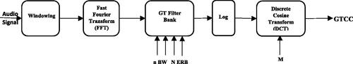
The GTCC filter bank depends on factors such as total filter bank bandwidth, GTCC filter sequence, the ERB (Equivalent Rectangular Bandwidth) energy model, and a handful of filters. The foundation of the ERB model is the notion that the human ear may be represented as a bank of band-pass filters that divide incoming sounds into various frequency bands. The auditory system’s processing of these frequency ranges, which results in the perception of speech sounds, is then simulated by the model. The ERB model can be used to extract particular properties from speech signals that can be utilized to distinguish individual speakers, which is relevant to speaker recognition. These characteristics can include a person’s voice’s pitch and formant frequencies, as well as other characteristics of their speech patterns. The default gammatone filter bank is made up of gammatone filters spaced linearly on the ERB scale from 50 to 8000 Hz. Finally, the log function and the DCT are used to model human loudness perception and decorrelate the logarithmically compressed filter outputs, resulting in better power compaction (Abdulla and Yushi 2010). The overall computation cost is roughly equivalent to the MFCC computation. See Figure 2: Block diagram describing the computation of the adapted Gammatone cepstral coefficients (Abdulla and Yushi 2010).

Figure 2. Block diagram describing the computation of the adapted Gammatone cepstral coefficients.

2.6.2.1. Windowing

Extraction of the best parametric representation of acoustic signals is a critical task for improving recognition performance. The efficiency of this phase is critical for the next phase because it influences its behavior. The audio samples are first windowed (using a Hamming window) into 30 ms frames with a 15 ms overlap (Abdulla and Yushi 2010).

The frequency range for analysis is set to 20 Hz (the lowest audible frequency) to the Nyquist frequency (in this work, 11 KHz). This process serves two purposes: This process serves two purposes (Abdulla and Yushi 2010):

1. the (typically) non-stationary audio signal can be assumed to be stationary for such a short interval, making spectrotemporal signal analysis easier; and

2. The efficiency of the feature extraction process is increased.

The Hamming window equation is given as:

If the window is defined as $W(n),0\le n\le N-1$

Where;

N = number of samples in each frame Y[n] = Output signal

X(n) = input signal

W(n) = Hamming window, then the result of the windowing signal is shown in Equation (2.7a(2.7a) $$\begin{array}{l}Y(n)=X(n)\ast W(n)\end{array}$$(2.7a) ): (2.7a) $$\begin{array}{l}Y(n)=X(n)\ast W(n)\end{array}$$(2.7a)

Where W(n) is expressed in (2.7b(2.7b) $$\begin{array}{l}W(n)=0.54-0.46\cos [2\mathrm{\Pi n}/N-1]\text{ For }0\le n\le N-1\end{array}$$(2.7b) )

(2.7b) $$\begin{array}{l}W(n)=0.54-0.46\cos [2\mathrm{\Pi n}/N-1]\text{ For }0\le n\le N-1\end{array}$$(2.7b)

2.6.2.2. The GTCC filter bank

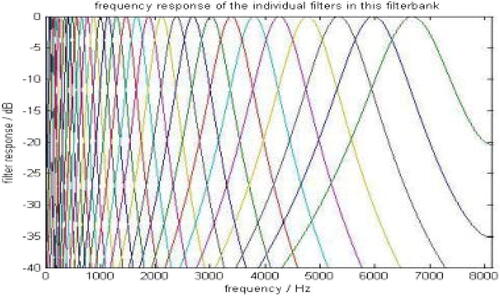
The GTCC filter bank is made up of the frequency responses of various GTCC filters. It is applied to the fast Fourier transform (FFT) of the signal, emphasizing perceptually meaningful sound signal frequencies. GTCC Filter Bank output is displayed in Figure 3.

Figure 3. GTCC filter bank output (Abdulla and Yushi 2010 ).

2.6.2.3. Fast Fourier transform (FFT)

Each frame of N samples is converted from the time domain to the frequency domain as defined in (2.8(2.8) $$\begin{array}{l}Y(w)=\mathrm{FFT}[h(t)\ast X(t)]=H(w)\ast X(w)\end{array}$$(2.8) ). (2.8) $$\begin{array}{l}Y(w)=\mathrm{FFT}[h(t)\ast X(t)]=H(w)\ast X(w)\end{array}$$(2.8)

For X(w), H(w)andY(w) is the Fourier Transform of X(t), H(t)andY(t), respectively.

2.7. Review of related works

Kadiri and Alku worked on “Analysis and Detection of Pathological Voice Using Glottal Source Features” (Kadiri and Alku 2020), where they tried to give a systematic analysis of global source features as investigations into voice pathology detection were carried on. Several authors have established some illnesses are capable of altering human voices, and this poses a great challenge to recognizing a person by the sound of their voice. Z. Luo et al. (Luo et al. 2019), work on “Emotional Voice Conversion Using Dual Supervised Adversarial Networks With Continuous Wavelet Transform F0 Features” where they propose an adaptive scale ceaseless wavelet transform (ADS-CWT) method to systematically capture F0 features of different temporal levels, which can represent different speech mannerism aspects, ranging from micro-prosody to a full-blown sentence. Sizov et al. (Sizov et al. 2015), were motivated to do this work by the vulnerability of virtually all speaker recognition systems to spoofing. The authors, here, focused on Voice Conversion (VC) which happens to be one of the most challenging aspects of modern voice recognition systems in detecting spoofing. Tandel et al. (2020) investigated voice recognition and a comparison of voices using machine learning. The authors highlighted some of the variants of voice recognition as it concerns speaker recognition and also hinted at several approaches to voice comparison. S. Ding et al. (Ding et al. 2020), proposed a technique called Cluster-Structured Sparse Representation (CSSR) which improves speaker independence of the dictionary representation with a more efficient voice conversion. The authors conducted four experiments on the CMU ARCTIC corpus to evaluate their proposed representation technique. Zhang et al. (Zhang et al. 2020), present a sequence-to-sequence voice conversion using non-parallel training data. The authors built their model on the framework of encoder-decoder neural networks. The paper presented a recognition encoder that was designed to learn disentangled linguistic representations with data training and adversarial training strategies.

In all of the works so far relating to voice recognition, none of the researchers have worked on datasets of varying languages or voices from African localities. In this work, we have developed a novel feature extraction algorithm that competes favorably with the likes of MFCC and GTCC. Our approach addresses the recognition that has to do with bilingual persons and the accuracy of the performance of the machine. So many observations were made concerning their performance metrics. Works have been made using extracted features of MFCC (Ahmad et al. 2017; Alexander et al. 2018; Ariav and Cohen 2019; Bakowski and Muromtsev 2020; Ding et al. 2020; Ferrer et al. 2019; Iloanusi et al. 2019; Kadiri and Alku 2020; Kinkiri and Keates 2020; Partila et al. 2020; Perero-Codosero et al. 2020; Poddar and Saha 2017; Sajjad et al. 2020; Stastny et al. 2018; Tandel et al. 2020; Teo et al. 2020; Xu et al. 2022; Zhang et al. 2020) and GTCC (Ajimah et al. 2020; Grozdi’c and Slododan 2017; Vimala and Radha 2014).

3. Methodology

In this work, a novel feature extraction technique was proposed that was used for the recognition of individuals during the experimental stage. We also collected a novel voice dataset called AfroVoice in Nigeria that was collected in the northern and eastern regions of Nigeria- Kaduna State and Enugu State, to be precise. Voice is an efficient way of authenticating people, as this does not rely on what the individual says but can be used to distinctively tell individuals apart as well as figure out what an individual says. In this research work, we have built a voice recognition system, and more emphasis was placed on the feature extraction level. Several feature extraction algorithms were modelled, that were derived from Pitch and Mel Frequency Cepstral Coefficient (MFCC). The proposed feature extraction was designed from the concatenation of the power of the Gaussian Mathematical equation, Spherical Mathematical equation, and Electric Field Potential equation. The concatenation was horizontal for the Traditional approach.

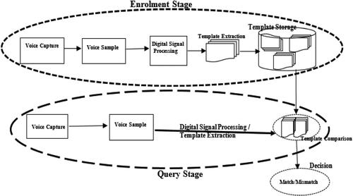
The experiment was performed in a MATLAB environment where several databases were experimented on to evaluate the performance of the proposed model. The experiment was done using the traditional approach of speaker recognition. The results of all of the approaches were compared with one another as well as the approaches embraced in voice authentication. In Section 3.2, we shall be discussing the derivation of the feature extraction models which we have proposed in this work. Figure 4 is a schematic diagram that illustrates a typical voice recognition system, figuratively showing the enrolment stage, storage database, and query phase. It also shows how the query voice template is compared with the stored voice template in the comparison module. The decision module now takes the action of either accepting or not accepting depending on the threshold level of the decision mechanism.

Figure 4. Schematic diagram of voice authentication system.

3.1. Proposed voice feature extraction models

In this work, a novel feature extraction model was derived from the MFCC, the GTCC, and Pitch. The proposed feature extraction technique is designed by the concatenation of the following mathematical models which are enlisted as follows;

1. Gaussian Power Features, ‘W’;

2. Spherical Features ‘Sp’;

3. Electric Field Potential ‘E_pt’.

Concatenation of (‘W’, ‘Sp’, ‘E_pt’) gives the extracted feature. The performance of this proposed feature extraction was compared with the MFCC, and the GTCC, as well as their differentials (delta) and accelerations (deltaDelta). The concatenation was made, and the salient features of voice extraction were used to feed the mathematical models, ‘W’, ‘Sp’, and ‘E_pt’

3.1.1. The Gaussian power model G (w)

The Gaussian normal distribution equation was modified to model feature extraction. The Gaussian distribution function can be used to explain physical occurrences if the number of participants is very large. A time-series function that estimates the exact binomial distribution of occurrences is the Gaussian distribution. The normalized Gaussian distribution presented has a probability of one (1) when the total of all x (The variable x in (3.1(3.1) $$\begin{array}{l}f\left(x\right)=\frac{1}{\sigma \sqrt{2\pi }}{e}^{\frac{-1}{2}{\left(\frac{\text{x}-\mu }{\sigma }\right)}^2}\end{array}$$(3.1) ) is a positive integer) values is taken. The Gaussian has a probability of being within one standard deviation of the mean of 0.683. A normal (or Gaussian, Gauss, or Laplace–Gauss) distribution for a real-valued random variable is a type of continuous probability distribution in probability theory. The probability density function’s general form is: (3.1) $$\begin{array}{l}f\left(x\right)=\frac{1}{\sigma \sqrt{2\pi }}{e}^{\frac{-1}{2}{\left(\frac{\text{x}-\mu }{\sigma }\right)}^2}\end{array}$$(3.1)

The Equation (3.1(3.1) $$\begin{array}{l}f\left(x\right)=\frac{1}{\sigma \sqrt{2\pi }}{e}^{\frac{-1}{2}{\left(\frac{\text{x}-\mu }{\sigma }\right)}^2}\end{array}$$(3.1) ) above was used to model the Gaussian model with some terms and equations that serve as helpers in understanding the functionality of this model. The fundamental features that were used in the formation of our models are the MFCC and GTCC coefficients, the delta, the delta-Delta, and the Pitch. We will, henceforth, derive our mathematically modeled equations for voice feature extraction. The MFCC coefficient was extracted, as were the Pitch and the delta-Delta features of the MFCC. The relevant portion of the equation for this model is the power of the Gaussian exponential as in Equation (3.2(3.2) $$\begin{array}{l}\mathit{\text{Gaussian Power, W}}=\frac{-1}{2}{\left(\frac{x-\mu }{\sigma }\right)}^2\end{array}$$(3.2) ), which is redesigned to extract some voice features derived from the MFCC voice features and the pitch voice feature extract. (3.2) $$\begin{array}{l}\mathit{\text{Gaussian Power, W}}=\frac{-1}{2}{\left(\frac{x-\mu }{\sigma }\right)}^2\end{array}$$(3.2)

The coefficients, the deltas, and, the delta-Deltas of MFCC G’s and GTCC’s of voices were extracted, converted to vector, and summed as J, in (3.3(3.3) $$\begin{array}{ll}J& =(\mathrm{GTC}{C}_c+\mathrm{GTC}{C}_d+\mathrm{GTC}{C}_{\mathrm{dD}})\\ & +(\mathrm{MFC}{C}_{\text{c}}+{\text{MFCC}}_d+\mathrm{MFC}{C}_{\mathrm{dD}})\end{array}$$(3.3) );

(3.3) $$\begin{array}{ll}J& =(\mathrm{GTC}{C}_c+\mathrm{GTC}{C}_d+\mathrm{GTC}{C}_{\mathrm{dD}})\\ & +(\mathrm{MFC}{C}_{\text{c}}+{\text{MFCC}}_d+\mathrm{MFC}{C}_{\mathrm{dD}})\end{array}$$(3.3)

Where; GTCC_c is the GTCC’s coefficient, the GTCC_d is the GTCC’s delta (i.e., first derivative) and GTCC_dD is the GTCC’s deltaDelta (i.e., second derivative). Similarly, MFCC_c is the MFCC’s coefficient, the MFCC_d is the MFCC’s delta and MFCC_dD is the MFCC’s deltaDelta.

The pitch f₀ extracted and the standard deviation is thus obtained as t in (3.4(3.4) $$\begin{array}{l}t=\sqrt{\frac{\sum \mathrm{\Delta }{f}_0^2}{N}}\end{array}$$(3.4) ) for N number of pitch variables. (3.4) $$\begin{array}{l}t=\sqrt{\frac{\sum \mathrm{\Delta }{f}_0^2}{N}}\end{array}$$(3.4)

T is the Root-Mean-Square of the standard deviation of the pitch, t and it is given as shown in (3.5(3.5) $$\begin{array}{l}T=\frac{t}{\sqrt{2}}\end{array}$$(3.5) );

(3.5) $$\begin{array}{l}T=\frac{t}{\sqrt{2}}\end{array}$$(3.5)

Thus; substituting $-(x-\mu {)}^2$ of the numerator of (3.2(3.2) $$\begin{array}{l}\mathit{\text{Gaussian Power, W}}=\frac{-1}{2}{\left(\frac{x-\mu }{\sigma }\right)}^2\end{array}$$(3.2) ) with J of (3.3(3.3) $$\begin{array}{ll}J& =(\mathrm{GTC}{C}_c+\mathrm{GTC}{C}_d+\mathrm{GTC}{C}_{\mathrm{dD}})\\ & +(\mathrm{MFC}{C}_{\text{c}}+{\text{MFCC}}_d+\mathrm{MFC}{C}_{\mathrm{dD}})\end{array}$$(3.3) ) and 2σ² of the denominator of (3.2(3.2) $$\begin{array}{l}\mathit{\text{Gaussian Power, W}}=\frac{-1}{2}{\left(\frac{x-\mu }{\sigma }\right)}^2\end{array}$$(3.2) ) with T of (3.5(3.5) $$\begin{array}{l}T=\frac{t}{\sqrt{2}}\end{array}$$(3.5) ) we now get the Gaussian Power Model, W, in (3.2(3.2) $$\begin{array}{l}\mathit{\text{Gaussian Power, W}}=\frac{-1}{2}{\left(\frac{x-\mu }{\sigma }\right)}^2\end{array}$$(3.2) ) is now rewritten as in (3.6(3.6) $$\begin{array}{l}\mathit{\text{Gaussian Power}},W(J,T)=\frac{J}{T}\end{array}$$(3.6) ). (3.6) $$\begin{array}{l}\mathit{\text{Gaussian Power}},W(J,T)=\frac{J}{T}\end{array}$$(3.6)

3.1.2. The spherical model S(J)

In this model, we used the spherical mathematical equation to model our voice feature extraction. The Spherical feature extraction model is given in (3.7(3.7) $$\begin{array}{l}S\left(r\right)=\frac{4}{3}\pi r^3\end{array}$$(3.7) );

(3.7) $$\begin{array}{l}S\left(r\right)=\frac{4}{3}\pi r^3\end{array}$$(3.7)

Substituting J in (3.3(3.3) $$\begin{array}{ll}J& =(\mathrm{GTC}{C}_c+\mathrm{GTC}{C}_d+\mathrm{GTC}{C}_{\mathrm{dD}})\\ & +(\mathrm{MFC}{C}_{\text{c}}+{\text{MFCC}}_d+\mathrm{MFC}{C}_{\mathrm{dD}})\end{array}$$(3.3) ) for r in (3.7(3.7) $$\begin{array}{l}S\left(r\right)=\frac{4}{3}\pi r^3\end{array}$$(3.7) ) to yield the spherical model which is shown in (3.8(3.8) $$\begin{array}{l}S\left(J\right)=\frac{4}{3}\pi J^3\end{array}$$(3.8) );

(3.8) $$\begin{array}{l}S\left(J\right)=\frac{4}{3}\pi J^3\end{array}$$(3.8)

Where J is defined in (3.8(3.8) $$\begin{array}{l}S\left(J\right)=\frac{4}{3}\pi J^3\end{array}$$(3.8) ). The sphere model is thus; S(J),

3.1.3. The electric field model potential E_pt(J, J_dD)

The Electric Field Model E_pt(J, J_dD), is based on Newton’s law of the electric field. An electric field is emitted by every charged object. This electric field is the source of the electric force experienced by other charged particles. A charge’s electric field exists everywhere, although its strength diminishes as the distance is squared. The electric field unit in SI is Newton per Coulomb (N∕s).

A test charge can be used to determine the Electric Field of a charged item. A test charge is a tiny charge that can be used to map an electric field at various locations. The test charge is designated as q0. An electric field exists at a given location if a test charge is placed there and experiences an electrostatic force. The electrostatic force at the test charge’s position is denoted by $\overrightarrow{F}$. See mathematical Equation (3.9(3.9) $$\begin{array}{l}\overrightarrow{F_0}=\frac{1}{4\pi {\epsilon }_0}\times \frac{\left|q{q}_0\right|}{r^2}\end{array}$$(3.9) ) for $\overrightarrow{F}$;

(3.9) $$\begin{array}{l}\overrightarrow{F_0}=\frac{1}{4\pi {\epsilon }_0}\times \frac{\left|q{q}_0\right|}{r^2}\end{array}$$(3.9)

From Equation (3.9(3.10) $$\begin{array}{l}\overrightarrow{F_0}=q\overrightarrow{E}\end{array}$$(3.10) ) it is possible to evaluate the magnitude of the electric field, $\overrightarrow{E}$;

(3.10) $$\begin{array}{l}\overrightarrow{F_0}=q\overrightarrow{E}\end{array}$$(3.10)

Where E is the electric field q and q0 the charges then $\frac{1}{4\pi {\epsilon }_0}$ is the constant, ε₀ is the permittivity of free space. Substituting Equation (3.9(3.9) $$\begin{array}{l}\overrightarrow{F_0}=\frac{1}{4\pi {\epsilon }_0}\times \frac{\left|q{q}_0\right|}{r^2}\end{array}$$(3.9) ) in Equation (3.10(3.10) $$\begin{array}{l}\overrightarrow{F_0}=q\overrightarrow{E}\end{array}$$(3.10) ) we obtain;

(3.11) $$\begin{array}{l}\overrightarrow{E_0}=\frac{1}{4\pi {\epsilon }_0}\times \frac{\left|q_o\right|}{r^2}\end{array}$$(3.11)

Electric field potential is E_pt is thus shown in (3.12a(3.12a) $$\begin{array}{l}{E}_{\text{pt}}=\overrightarrow{E_0}\times r\end{array}$$(3.12a) ) and (3.12b(3.12b) $$\begin{array}{l}{E}_{\text{pt}}=\frac{1}{4\pi {\epsilon }_0}\times \frac{\left|q_o\right|}{r}\end{array}$$(3.12b) );

(3.12a) $$\begin{array}{l}{E}_{\text{pt}}=\overrightarrow{E_0}\times r\end{array}$$(3.12a)

Substituting (3.11(3.11) $$\begin{array}{l}\overrightarrow{E_0}=\frac{1}{4\pi {\epsilon }_0}\times \frac{\left|q_o\right|}{r^2}\end{array}$$(3.11) ) in (3.12a(3.12a) $$\begin{array}{l}{E}_{\text{pt}}=\overrightarrow{E_0}\times r\end{array}$$(3.12a) ) we get (3.12b(3.12a) $$\begin{array}{l}{E}_{\text{pt}}=\overrightarrow{E_0}\times r\end{array}$$(3.12a) )

(3.12b) $$\begin{array}{l}{E}_{\text{pt}}=\frac{1}{4\pi {\epsilon }_0}\times \frac{\left|q_o\right|}{r}\end{array}$$(3.12b)

The sum of deltaDelta of GTCC_dDandMFCC_dD is given by J_dD and it is expressed mathematically as in (3.13(3.13) $$\begin{array}{l}{J}_{\mathrm{dD}}=\mathrm{GTC}{C}_{\mathrm{dD}}+\mathrm{MFC}{C}_{\mathrm{dD}}\end{array}$$(3.13) )

(3.13) $$\begin{array}{l}{J}_{\mathrm{dD}}=\mathrm{GTC}{C}_{\mathrm{dD}}+\mathrm{MFC}{C}_{\mathrm{dD}}\end{array}$$(3.13)

Replacing the constant, $\frac{1}{4\pi {\epsilon }_0}$ with $\frac{1}{4\pi }$ by assuming ε₀ to be unity such that it will not affect the entire equation systematically, then, substituting J_dD in Equation (3.13(3.13) $$\begin{array}{l}{J}_{\mathrm{dD}}=\mathrm{GTC}{C}_{\mathrm{dD}}+\mathrm{MFC}{C}_{\mathrm{dD}}\end{array}$$(3.13) ) for r in (3.12b(3.12b) $$\begin{array}{l}{E}_{\text{pt}}=\frac{1}{4\pi {\epsilon }_0}\times \frac{\left|q_o\right|}{r}\end{array}$$(3.12b) ) and J in (3.7(3.7) $$\begin{array}{l}S\left(r\right)=\frac{4}{3}\pi r^3\end{array}$$(3.7) ) for $\left|q_o\right|$ in (3.12b(3.12b) $$\begin{array}{l}{E}_{\text{pt}}=\frac{1}{4\pi {\epsilon }_0}\times \frac{\left|q_o\right|}{r}\end{array}$$(3.12b) ) we obtain (3.14(3.14) $$\begin{array}{l}{E}_{\mathrm{pt}}(J,J_{\mathrm{dD}})=\frac{1}{4\pi }\times \frac{J}{J_{\mathrm{dD}}}\end{array}$$(3.14) )

(3.14) $$\begin{array}{l}{E}_{\mathrm{pt}}(J,J_{\mathrm{dD}})=\frac{1}{4\pi }\times \frac{J}{J_{\mathrm{dD}}}\end{array}$$(3.14)

Equation (3.14(3.14) $$\begin{array}{l}{E}_{\mathrm{pt}}(J,J_{\mathrm{dD}})=\frac{1}{4\pi }\times \frac{J}{J_{\mathrm{dD}}}\end{array}$$(3.14) ) is the electrical field E_pt(J, J_dD), the mathematical model for voice feature extraction.

So far we have four mathematical models proposed to extract voice features. Table 1 is a summary that shows all the voice feature extractor models for this work.

Table 1. Summary of proposed mathematical models concatenated for voice feature extraction.

S/N	Proposed model	Symbol	Mathematical equation
1	The Gaussian Power Model	𝐖(𝐉, 𝐓)	$\mathit{\text{GaussianPower}},W=\frac{J}{T}$
2	The Spherical Model	𝐒(𝐉)	$S\left(J\right)=\frac{4}{3}\pi J^3$
3	The Electric Field Potential Model	Ept(J, JdD)	$E_{\mathrm{pt}}(J,J_{\mathrm{dD}})=\frac{1}{4\pi }\times \frac{J}{J_{\mathrm{dD}}}$

The voice feature as proposed was used in the identification of speakers during the experiment. For the traditional method, the features are concatenated to be in a single vector of length 42 (i.e., $14\ast 3=42$).

3.1.4. Algorithm for feature extraction

The feature is extracted from the n-number of voice utterances, thus the algorithm for the feature extraction is as follows:

1. Extract MFCC Features, to get ${\left\{C_{\mathrm{mfcc}},d_{\mathrm{mfcc}},d{D}_{\mathrm{mfcc}}\right\}}_{f=1}^{f=n}$ and take their respective Standard deviations to get ${\left\{{\omega }_{\mathrm{mfcc}},{\lambda }_{\mathrm{mfcc}},{\phi }_{\mathrm{mfcc}}\right\}}_{f=1}^{f=n}$

2. Extract GTCC Features, to get ${\left\{C_{\mathrm{gtcc}},d_{\mathrm{gtcc}},d{D}_{\mathrm{gtcc}}\right\}}_{f=1}^{f=n}$ and take their respective Standard deviations to get ${\left\{{\omega }_{\mathrm{gtcc}},{\lambda }_{\mathrm{gtcc}},{\phi }_{\mathrm{gtcc}}\right\}}_{f=1}^{f=n}$

3. Extract the Pitch feature, f_o and compute the standard deviation to get t.

4. PERFORM sum(ω_mfcc&ω_gtcc) to get ${\left\{C_s\right\}}_{f=1}^{f=n}$

5. PERFORM sum (λ_mfcc&φ_mfcc) to get ${\left\{D_m^{\prime }\right\}}_{f=1}^{f=n}$

6. PERFORM sum (λ_gtcc&φ_gtcc) to get ${\left\{D_g^{\prime }\right\}}_{f=1}^{f=n}$

7. PERFORM sum ($C_s,D_m^{\prime }\mathrm{\&}{D}_g^{\prime })$ to get ${\left\{F_T^{\prime }\right\}}_{f=1}^{f=n}$

8. CALCULATE $F_T^{\prime }÷(\sqrt{2}\ast \mathrm{mean}(t)$ to get {modified Gaussian $\text{power},G_f{\}}_{f=1}^{f=n}$

9. CALCULATE $(4\ast \mathrm{Pi}\ast F_T^{\prime 3})÷3$ to get {Spherical Features, $S_f{\}}_{f=1}^{f=n}$

10. CALCULATE $(F_T^{\prime }\ast 4\ast \mathrm{pi}\ast \mathrm{mean}(D_m^{\prime }){)}^{-1}$ to get {Gravitational $\text{potential feature},G_{\mathrm{pf}}{\}}_{f=1}^{f=n}$

11. PERFORM horizontal concatenation of $(G_f,S_f\mathrm{\&}{G}_{\mathrm{pf}})$ $\mathrm{to}\mathrm{get}{\left\{\mathrm{feature}A\right\}}_{f=1}^{f=n}$ Feature A used for the traditional method.

12. PERFORM horizontal concatenation for (mean(ω_mfcc), $\mathrm{mean}({\lambda }_{\mathrm{mfcc}})\mathrm{\&}\mathrm{mean}({\phi }_{\mathrm{mfcc}}))\mathrm{to}\mathrm{get}{\left\{\mathrm{feature}C\right\}}_{f=1}^{f=n}$ Feature C is used for the traditional method.

13. PERFORM horizontal concatenation for (mean(ω_gtcc), $\mathrm{mean}({\lambda }_{\mathrm{gtcc}})\mathrm{\&}\mathrm{mean}({\phi }_{\mathrm{gtcc}}))\mathrm{to}\mathrm{get}{\left\{\mathrm{feature}D\right\}}_{f=1}^{f=n}$ Feature D is used for the traditional method.

14. PERFORM horizontal concatenation for $(C_s,D_m^{\prime }\mathrm{\&}{D}_g^{\prime })$ $\mathrm{to}\mathrm{get}{\left\{\mathrm{feature}E\right\}}_{f=1}^{f=n}$ Feature E is used for the traditional method.

3.2. Databases preparation

The experiments were performed on three databases namely; UNN-BVC-voice DB, AfroVoices-DB, and LibriSpeech-DB. The above-mentioned databases that were used in running this experiment of voice recognition will be discussed in the proceeding sub-sections.

3.2.1. LibriSpeech database

The LibriSpeech is a rich and well-stocked voice database that consists of datasets of both clean and some quite noisy data of subjects across the globe. For this experiment, we selected the voice sample of 40 speakers with 60 impressions each which were sorted into two sectional sets for Set-I and Set-II. The total number of impressions for the Set-I and Set-II we used happens to be 1200 impressions.

3.2.2. AfroVoices databases

This is a novel dataset that was collected in Nigeria across varying ethnicities in the country. The speaker was asked to say five (5) short utterances in English and was translated to vernacular, which makes it a total of ten (10) impressions per subject. Audacity is a free and open-source digital audio editor and recording software for Windows, macOS, Linux, and other Unix-like operating systems.

3.2.3. UNN-BVC voice database

This voice dataset comprises 3980 voice utterances that were acquired from 520 subjects of Nigerian descent (Iloanusi et al. 2019). The subjects are made up of 326 male and 194 female subjects with 1964 and 2016 voice utterances, respectively. Five short speeches were in English and were translated into five native Nigerian languages. Many females participated in the second session hence their samples were larger in number. In this research experiment, we prepared our dataset by selecting 176 subjects from the vernacular utterances with 5 impressions each, which sums up to 880 utterances, and for the English language, we selected 177 subjects with 5 short sentences each, which totals 885 utterances for the English language (Iloanusi et al. 2019).

3.3. Matching of the extracted features

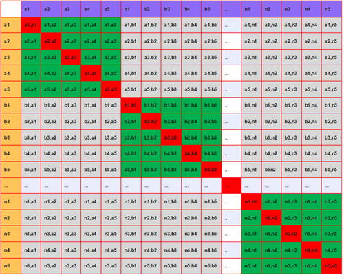
The features extracted are used to perform the evaluation directly for the traditional approach. The extracted features, which are in vector arrays, are compared which returns dissimilarity match-scores of matrix arrays of length n₅ by n₅, where n is the number of subjects and the subscript ’5’ indicates the number of utterances per subject. Figure 5 demonstrates the matching of n-numbers of subjects with five utterances each being cross-matched, the red boxes indicate self-match scores, the grey boxes indicate impostor match scores, and, the green boxes depict the genuine match scores. The accepted scores were matched with the avoidance of self-match, which happens to be along the main diagonal and is painted red, see Figure 5. The top and bottom triangles of the leading diagonal are mirror replicates thus, either the upper side or lower were selected as the regions of interest, and hence the genuine and impostor score matches could be deciphered. The genuine dissimilarity match scores are scores from the same subject except for the same utterance. Impostor dissimilarity match scores are scores that result from matching features from different subjects. The match scores of ‘a1’ to ‘a1’, ‘a2’ to ‘a2’, ‘b1’ to ‘b1’, ‘b2’ to ‘b2’, and so on will be discarded because they are dissimilarity self-match scores that happen to be zero (‘0’) and were neither classified as genuine nor impostor scores. The match scores of ‘a1’ to ‘a2 through 5’, ‘b1’ to ‘b2 through 5’, and so on, provided they are from the same subject, are dissimilarity genuine scores, else any match scores that result from a different subject is the dissimilarity impostor score. The dissimilarity scores are converted to similarity scores and the following parameters are obtained

1. Area Under Curve (AUC),

2. Genuine Acceptance Rate (GAR),

3. False Rejection Rate (FRR),

4. False Acceptance Ratio (FAR),

5. Equal Error Rate (EER)

The grey region is the unwanted portion of the match scores as it consists of the mirror values of the scores, at the upper diagonal, and the self-match scores (scores along the main diagonal) which are irrelevant in this case.

Figure 5. Arrays showing n-numbers of subjects being cross-matched, the red boxes across the diagonal indicate self-match scores, the grey boxes indicate impostor match scores, and, the green boxes depict the genuine match scores.

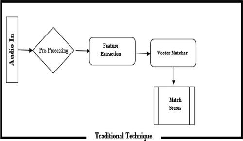
3.4. Voice recognition system using traditional approach

This approach has to do with the extraction of the acoustic features from the speech signal, followed by an estimation of the likelihood, and the match scores; genuine and impostor are then evaluated (Iloanusi and Osuagwu 2014). The audio input is processed and salient features are extracted. This extracted feature of utterances from several subjects is then matched (see Figure 6). The resulting scores tell if they are matched or mismatched. The matched scores tell which utterance is falsely or truly matched. If an utterance is matched with another utterance(s) from the same subject with score(s) above the threshold of the voice recognition system it accepts it (is a Genuine acceptance) else it rejects it (is falsely rejected). Also, if utterances from different subjects match with scores lower than the threshold the system rejects (true rejection) else the system accepts it (false acceptance).

Figure 6. Block diagram of voice recognition system using the Traditional technique.

3.4.1. Algorithm for the traditional approach

The algorithm for the Voice Recognition System Experiment using the Traditional method is as follows;

1. Extract features.

2. Match the extracted features to get the dissimilarity match scores.

3. Discard the scores on the leading diagonal of the match score as they result from self-matches.

4. Use the score of either the upper or lower triangle of the leading diagonal, as they are the same.

5. Get the genuine and impostor scores.

6. Convert the dissimilarity scores to similarity scores.

7. Compute the AUC and the EER.

3.5. Performance evaluation

The performance metrics used to measure the accuracy of this work are listed below;

1. The area under ROC (AROC) otherwise called the Area Under Curve (AUC),

2. Bar Chart,

3. Equal Error Rate (EER),

4. Experimental section

The experiment was performed on three databases (the AfroVoice database, the LibriSpeech database, and the UNN-BVC-voice database). The experiment was performed in two different approaches, namely, the traditional approach of speaker recognition. The features extracted for the experiment are shown in the summary of Table 2.

Table 2. Summary of the experimented features used the traditional approach and their components.

Proposed	Components of the feature	Sequence vector
features		length
A	Horizontal concatenation of Gaussian Model, Spherical model, and Electric Field Potential Model.	42
B	MFCC features: horizontal concatenation of the coefficient Delta and deltaDelta	42
C	GTCC features: horizontal concatenation of the coefficient Delta and deltaDelta	42
D	Horizontal concatenation of the sum of coefficients, the sum of the delta, and the sum of deltaDelta of MFCC and GTCC	42

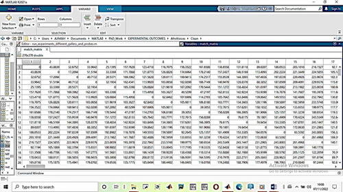
4.1. Voice recognition using traditional approaches

The features that were used in this approach constitute a single sequence vector that was extracted for different feature types, as summarized in Table 2. The empirical study was performed on three databases as discussed previously. Section 3 describes the matching algorithms of the experiments, and Figure 7 is a screenshot from the experimental outcome of the Match matrix showing dissimilarity scores that were performed in the MATLAB environment. The leading diagonals are zero which was a result of the self matches which indicates that there is no dissimilarity in matching the feature vector from the exactly same utterance. The self-match utterance however is discarded as its outcome is not necessarily required for this experiment.

Figure 7. Match matrix scores showing dissimilarity scores with the leading diagonals (zero) resulting from the self-matches.

4.1.1. Experimental results from AfroVoices

An experiment was performed on the AfroVoice Clean and Noisy databases of the English and the vernacular utterances and results were displayed to investigate the performances of voice recognition of these features as used on the database. The results are presented using the Area under the Receiver Operating Characteristic Curve (AROC) and Equal Error Rate (EER). As discussed in the previous section, a perfect AROC has a value of 1 and the curve tends to the upper vertical axis of the graph, and vice versa for a poor system. The perfect system has an EER is approximately 0%, which is to say the closer the EER of a system is to zero the better the system. A good DET tends towards the bottom left corner of the graph. At the end of the experiments, the following results were obtained AUC (or AROC) and EER is the metrics used in the performance evaluation.

4.2. Experimental analysis

The remaining sections and their successive sub-sections in this section have analyzed the performances of the experiments performed for speaker recognition using traditional. This report was based on the experimental outcomes performed on three databases; AfroVoices, LibriSpeech, and UNN_BVC.

4.3. Experimental result analysis using traditional method of voice verification

The experiment was performed on three datasets, namely, the AfroVoices (dataset built during this research), the LibriSpeech dataset, and the UNN-BVC dataset. Features A, B, C, and D were extracted for performance evaluation in the MATLAB environment. The detailed properties of the features are summarized in Table 2. The analysis of the experiments performed on the three databases used has been summarized in tables in sections and sub-sections.

4.3.1. Analysis of the AfroVoice experiment using the traditional method of voice verification

Experiments conducted on AfroVoice using the traditional technique of voice verification are summarized in Tables 3 and 4. These experiments were performed in two stages of data variation (the clean and the noisy). The tables also show the Equal Error Rate (EER) and Area under Curve (AUC or AROC) of the English and vernacular utterances of both variants. The performance of the vernacular is the same as the English-spoken data.

Table 3. Result analysis of AfroVoice (clean utterance) experiment.

Clean Afrovoice	English		Vernacular
Feature	AUC	EER	AUC	EER
A	0.68766	37.9686	0.68766	37.9686
B	0.69642	27.6827	0.69642	27.6827
C	0.66549	30.6331	0.66549	30.6331
D	0.57145	39.9686	0.57145	39.9686

Table 4. Result analysis of AfroVoice (noisy utterance) experiment.

Noisy Afrovoice	English		Vernacular
Feature	AUC	EER	AUC	EER
A	0.57021	38.7910	0.57021	38.7910
B	0.66862	28.8981	0.66862	28.8981
C	0.69405	28.7077	0.69405	28.7077
D	0.56731	35.2744	0.56731	35.2744

4.3.2. Analysis of LibriSpeech experiment using traditional method of voice verification

Experiments conducted on LibriSpeech using the traditional technique of voice verification were summarized in Table 5. These experiments were performed in two as the dataset was divided into two sets (SET-I and SET-II). The table also shows the Equal Error Rate (EER) and Area under Curve (AUC or AROC) of the SET-I and SET-II utterances (Panayotov et al. 2015).

Table 5. Result analysis of LibriSpeech database experiment.

LibriSpeech	Set I		Set-II
Feature	AUC	EER	AUC	EER
A	0.81572	36.0083	0.79989	38.5083
B	0.83229	21.1707	0.84974	23.6615
C	0.8528	19.9271	0.86302	22.0493
D	0.79334	25.5581	0.78167	24.9978

4.3.3. Analysis of UNN_BVC experiment using traditional method of voice verification

Experiments conducted on UNN_BVC using the traditional technique of voice verification were summarized in Table 6. These experiments were performed in two as the dataset was divided into two sets (English and Vernacular). The table also shows the Equal Error Rate (EER) and Area under Curve (AUC or AROC) of the two stages of the experiments based on their utterances.

Table 6. Result analysis of UNN-BVC database experiment.

UNN_BVC	English		UNN_BVC
Feature	AUC	EER	AUC	EER
A	0.7352	40.8954	0.82771	35.7347
B	0.6594	40.0788	0.68668	26.6491
C	0.6594	40.0788	0.70723	24.3254
D	0.6307	44.4293	0.61503	38.9676

4.3.4. Percentage change in performance due to noisy data

The analysis of the effect of noise on the performance of a voice biometric system is in Table 7. The change is defined as the ratio of the positive difference between the equal error rate, EER, of the noisy and the clean data to the largest value of the EER. The proposed feature, in this research, is least affected by noisy voice signals.

Table 7. Percentage change in performance due to noisy data experiment of AfroVoices.

Feature	EER-clean data	EER-noisy data	Change	Change (%)
A	37.9686	38.791	0.8224	2.12
B	27.6827	28.8981	1.2154	4.21
C	30.6331	28.7077	1.9254	6.25
D	39.9686	35.2744	4.6947	11.75

4.3.5. Discussion

The outcome of the experiment performed on the AfroVoices of clean and noisy databases is shown in Tables 3 and 4. The performance from the metrics AUC and EER shows that the results of the experiment on the English and Vernacular datasets are the same. The performance as observed in all of the features for A, B, C and, D have AUC; 0.68766, 0.69642, 0.66549 and, 0.57145 and EER: 37.9686, 27.6827, 30.6331, and 39.9686, respectively. For the noisy AfroVoice data, the performance metrics as observed in Table 4, AUC, and EER show that the results of the experiment on the English and Vernacular datasets are also the same. The performance as observed in all of the features for A, B, C, and, D have AUC; 0.57021, 0.66862, 0.69405 and, 0.56731 and EER: 38.7910, 28.8981, 28.7077 and. 35.2744, respectively, Result on Table 5 is quite improved compared with that of Tables 3 and 4. Table 6 is the outcome of the experiment on the UNN_BVC database.

5. Conclusion

Voice recognition is a means of identifying and verifying individuals by their voices, which has been employed recently in so many electronic systems and devices as access control. A voice-controlled device or system is faced with several challenges which could result in the misidentification of an individual. A failed or malfunctioning voice biometric system could lead to access denial of a genuine person from accessing facilities that they legally have access to and it could also grant an unauthorized impostor to gain access to a facility. Furthermore, when a voiceprint is misidentified in a crime scene it could result in injustice as the innocence will be misjudged as guilty and the guilty becomes innocent.

Voice as a modality in identifying an individual is susceptible to so many attacks such as voice mimicry, audio playback and voice-cloning, also known as audio deepfake, it is an artificial intelligence product employed to generate an audio sentence that sounds like a specific person. Deepfake is one of the greatest concerns to researchers across the universe, as it has the potential to promote false news (rumors), domestic violence, identity theft and social unrest.

From the result of the experiment performed in the AfroVoice DB, the proposed feature extraction model competed favorably with the analysis done in the table. The experiment that was repeated in two other databases shows that there is a significant improvement in the entire system as the number of subjects tends to grow. The better performance observed in the experimentation on the Librispeech dataset was a result of the nature of the dataset cleanliness over a noisier Afrovoices and UNN-BVC. Datasets. The experiment on the UNN-BVC shows that the proposed feature extractor, A, outperforms the other feature extractors both in English and the vernacular. Results from the experiment performed on the English UNN-BVC, the proposed model has an AUC score of 74% against 66%, 66%, and 63% for the MFCC, GTCC, and combination of MFCC and GTCC, respectively. Results from the experiment performed on the vernacular-UNN-BVC, the proposed model has an AUC score of 83% against 69%, 71%, and 62% for the MFCC, GTCC, and combination of MFCC and GTCC, respectively. Percentage change in performance due to noisy data is lowest in the proposed feature extraction in this paper with a value of 2.12% as compared with features B, C, and D which are 4.21%, 6.25%, and 11.75%. respectively. The proposed voice feature extractor is more stable to noise. Our proposed concatenated feature happens to be more stable to noisy voice data when compared with other voice features (B, C, and D) in competition. The experiment on the Afrovoice data set shows that there are no discrepancies between the performances on the English and Vernacular datasets. The performance on clean data is higher on the clean data as compared with the noisy datasets.

5.1. Recommendation and future work

This work has been done in three databases, but quite a few recommendations have been enclosed in this list for better work in the future. Below are some of the recommendations for future work:

1. For better performance in the machine learning approach, we recommend a well-stocked voice dataset collection of about 5000 subjects and 20 impressions each.

2. A build-up of an exceptional novel voice feature extractor that is independent of the traditional voice feature extractors, like MFCC, GTCC, or iVector.

3. We recommend running the experiment on a huge dataset to determine the generality of the performance of the voice recognition system.

4. We recommend that in the future, the ML experimental approach be carried out using the CNN and its performance compared to that of the BiLSTM approach.

5. We recommend the experiment be performed on a mimicry dataset and that a comparison of the performance with other existing approaches be statistical.

6. We recommend running the experiment on an entirely disjointed training dataset from the testing dataset and comparing its performances.

Disclosure statement

We have not received any form of grant or funding from any external source in executing this research. We have not by any means got any writing assistant outside the authors on this paper. This research is purely self-sponsored by the authors.

Data availability statement

The data relating to this subject can be found in the following links:

1. The UNN_BVC dataset is available at (https://doi.org/10.1109/ISCMI47871.2019.9004306) or contact the corresponding author via mail.

2. The LibriSpeech dataset could be requested from the corresponding of this linked journal https://ieeexplore.ieee.org/document/7178964

References

- Abdulla WH, Zhang Y. 2010. Voice biometric feature using Gammatone filterbank and ICA. Int J Biometr. 2:330–349.
- Ahmad N, Helmy M, Wahab A, Verma G, Sinha A. 2017. Motorcycle start-stop system based on intelligent biometric voice recognition. Mater Sci Eng. 6: 1–8. 10.1088/1742-6596/755/1/011001.
- Ajimah EN, Iloanusi ON, Eze MC, Olisa S. 2017. Adaptive encryption technique to protect biometric template in biometric database using a modified Gaussian function. Int J Sci Eng Res. 8:722–734.
- Ajimah, NE, N, Ezukwoke, IC, Dialoke, A, Odaba, ON, Iloanusi, 2020. Overview of voice biometric systems: voice person identification and challenges. LGT-ECE_UNN International Conference: Technological Innovation for Holistic Sustainable Development (TECHISD2020), p. 57–62.
- Alexander D, Thomsen L, Hautam RG, Kinnunen T, Tan Z, Member S, Parts R, Pitk M. 2018. Robust voice liveness detection and speaker verification using throat microphones. IEEE/ACM Trans Audio Speech Lang Process. 26:44–56.
- Ariav I, Cohen I. 2019. An end-to-end multimodal voice activity detection using wavenet encoder and residual networks. IEEE J Sel Top Signal Process. 13:265–274. 10.1109/JSTSP.2019.2901195.
- Bakowski, P, Muromtsev, D, 2020. On voice autentication algorithm development. CEUR Workshop Proceedings, 2590:1– 7.
- Bao X, Zhu J. 2012. A novel voice activity detection based on phoneme recognition using statistical model. J Audio Speech Music Proc. 2012:1–10. 10.1186/1687-4722-2012-1.
- Bisio I, Garibotto C, Grattarola A, Lavagetto F, Sciarrone A. 2018. Smart and Robust Speaker Recognition for Context-Aware In-Vehicle Applications. IEEE Trans Veh Technol. 67:8808–8821. 10.1109/TVT.2018.2849577.
- Ding S, Zhao G, Liberatore C, Gutierrez-Osuna R. 2020. Learning structured sparse representations for voice conversion. IEEE/ACM Trans Audio Speech Lang Process. 28:343–354. 10.1109/TASLP.2019.2955289.
- Dişken G, Tüfekci Z, Çevik U. 2017. A robust polynomial regression-based voice activity detector for speaker verification. J Audio Speech Music Proc. 2017:1–16. 10.1186/s13636-017-0120-6.
- Ferrer L, Nandwana MK, McLaren M, Castan D, Lawson A. 2019. Toward fail-safe speaker recognition: trial-based calibration with a reject option. IEEE/ACM Trans Audio Speech Lang Process. 27:140–153. 10.1109/TASLP.2018.2875794.
- Grozdi’C TG, Slododan TJ. 2017. Whispered speech recognition using deep denoising autoencoder and inverse filtering. IEEE/ACM Trans Audio Speech Language Process. 25:2313–2322.
- Guan W. 2018. Performance optimization of speech recognition system with deep neural network model. Opt. Mem. Neural Netw. 27:272–282. 10.3103/S1060992X18040094.
- Hansen JHL, Hasan T. 2015. Speaker recognition by machines and humans: a tutorial review. IEEE Signal Process Mag. 32:74–99. 10.1109/MSP.2015.2462851.
- Iloanusi O, Ejiogu U, Okoye IE, Ezika I, Ezichi S, Osuagwu C, Ejiogu E. 2019. Voice recognition and gender classification in the context of native languages and lingua franca. 6th International Conference on Soft Computing and Machine Intelligence 2019, 175–179. 10.1109/ISCMI47871.2019.9004306
- Iloanusi ON, Osuagwu CC. 2014. Fingerprint indexing based on minutiae-dependent statistical codes. Int. J. Electron. 101:950–962. 10.1080/00207217.2013.805384.
- Ismail M, Memon S, Dhomeja LD, Shah SM, Hussain D, Rahim S, Ali I. 2021. Development of a regional voice dataset and speaker classification based on machine learning. J Big Data. 8:1–18. 10.1186/s40537-021-00435-9.
- Kadiri SR, Alku P. 2020. Analysis and detection of pathological voice using glottal source features. IEEE J Sel Top Signal Process. 14:367–379. 10.1109/JSTSP.2019.2957988.
- Kinkiri S, KeatesS. 2020, Speaker identification: variations of a human voice. IEEE: International Conference on Advanced Computing & Communication Systems (ICACCS) Voice, 20: 18–21.
- Latinus M, Belin P. 2011. Human voice perception. Curr Biol. 21:R143–145. 10.1016/j.cub.2010.12.033.
- Luo Z, Chen J, Takiguchi T, Ariki Y. 2019. Emotional voice conversion using dual supervised adversarial networks with continuous wavelet transform F0 features. IEEE/ACM Trans Audio Speech Lang Process. 27:1535–1548. 10.1109/TASLP.2019.2923951.
- Maltoni, D, Maio D, Jaint AK, Prabhakar S. 2009. Handbook of Fingerprint Recognition. 2nd ed. London: Springer-Verlag.
- Ortega-Garcia J, Fierrez J, Alonso-Fernandez F, Galbally J, Freire MR, Gonzalez-Rodriguez J, Garcia-Mateo C, Alba-Castro J-L, Gonzalez-Agulla E, Otero-Muras E, et al. 2010. The multiscenario multienvironment BioSecure Multimodal Database (BMDB). IEEE Trans Pattern Anal Mach Intell. 32:1097–1111.
- Pal M, Paul D, Saha G. 2018. Synthetic speech detection using fundamental frequency variation and spectral features. Comput. Speech Lang. 48:31–50. 10.1016/j.csl.2017.10.001.
- Panayotov, V, Chen G, Khudanpur DSP. 2015. Librispeech: An ASR corpus based on public domain audio books. IEEE International Conference on Acoustics, Speech and Signal Processing, 5206–5210. https://ieeexplore.ieee.org/document/7178964.
- Partila P, Tovarek J, Ilk GH, Rozhon J, Voznak M. 2020. Deep learning serves voice cloning: how vulnerable are automatic speaker verification systems to spoofing trials?. IEEE Commun Mag. 58:100–105.
- Perero-Codosero JM, Espinoza-Cuadros F, Anton-Martin J, Barbero-Alvarez MA, Hernandez-Gomez LA. 2020. Modeling Obstructive Sleep Apnea Voices Using Deep Neural Network Embeddings and Domain-Adversarial Training. IEEE J Sel Top Signal Process. 14:240–250. 10.1109/JSTSP.2019.2957977.
- Poddar A, Saha G. 2017. Speaker verification with short utterances: a review of challenges, trends and opportunities. IET Biom. 7:91–101. 10.1049/iet-bmt.2017.0065.
- Ranjan R, Thakur A. 2019. Analysis of feature extraction techniques for speech recognition system. Int J Innov Technol Expl Eng (IJITEE). 8:197–200.
- Sajjad M, Kwon S, Soonil K. 2020. Clustering-based speech emotion recognition by incorporating learned features and deep BiLSTM. IEEE Access. 8:79861–79875. 10.1109/ACCESS.2020.2990405.
- Shrawankar U, Thakare VM. 2013. Techniques for feature extraction in speech recognition system: a comparative study. Int J Comput Appl Eng Technol Sci. 2:412–418.
- Sizov A, Khoury E, Kinnunen T, Wu Z. 2015. Joint speaker verification and anti-spoofing in the i-vector space. IEEE Trans Inf Forens Secur. 25:1–11. 10.1109/TIFS.2015.2407362.
- Stastny J, Munk M, Juranek L. 2018. Automatic bird species recognition based on birds vocalization. J Audio Speech Music Proc. 2018:1–8. 10.1186/s13636-018–0143-7.
- Tandel, NH, Prajapati HB, Dabhi VK. 2020. Voice recognition and voice comparison using machine learning techniques: a survey. IEEE International Conference on Advanced Computing & Communication Systems (ICACCS):459–465.
- Teo JH, Cheng S, Alioto M. 2020. Low-Energy Voice Activity Detection via Energy-Quality Scaling From Data Conversion to Machine Learning. IEEE Trans Circuits Syst I. 67:1378–1388. 10.1109/TCSI.2019.2960843.
- Tovarek J, Ilk GH, Partila P, Voznak M. 2018. Human Abnormal Behavior Impact on Speaker Verification Systems. IEEE Access. 6:40120–40127. 10.1109/ACCESS.2018.2854960.
- Trojahn M. 2012. Biometric authentication through a virtual keyboard for smartphones. Int J Comput Sci Inf Technol (IJCSIT). 4:1–12.
- Vimala C, Radha V. 2014. Suitable feature extraction and speech recognition technique for isolated tamil spoken words. Int J Comput Sci Inform Technol. 5:378–383.
- Xu Y, Wang W, Cui H, Xu M, Li M. 2022. Paralinguistic singing attribute recognition using supervised machine learning for describing the classical tenor solo singing voice in vocal pedagogy. EURASIP J Audio Speech Music. 2:16.
- Zhang J, Ling Z, Dai L. 2020. Non-parallel sequence-to-sequence voice conversion with disentangled linguistic and speaker representations. IEEE/ACM Trans Audio Speech Lang Process. 28:540–552. 10.1109/TASLP.2019.2960721.
- Zhang T, Shao Y, Wu Y, Pang Z, Member S. 2020. Multiple vowels repair based on pitch extraction and line spectrum pair feature for voice disorder. IEEE J Biomed Health Inform. 24:1940–1951. 10.1109/JBHI.2020.2978103.
- Zhang X, Cheng D, Jia P, Dai Y, Xu X. 2020. An efficient android-based multimodal biometric authentication system with face and voice. IEEE Access. 8:102757–102772. 10.1109/ACCESS.2020.2999115.