
 ?Mathematical formulae have been encoded as MathML and are displayed in this HTML version using MathJax in order to improve their display. Uncheck the box to turn MathJax off. This feature requires Javascript. Click on a formula to zoom.
ABSTRACT
In this paper, different numerical schemes are developed and investigated for solving singularly perturbed delay differential equations (DDEs). The solution of the considered equations exhibits a strong boundary layer when the perturbation parameter approaches zero. Standard numerical methods developed for solving regular problems fail to treat accurately the considered equations. We developed three numerical schemes for treating the considered equations. The first scheme (Scheme I) uses a non-standard mid-point upwind finite difference method on uniform mesh; the second scheme (Scheme II) uses a standard mid-point upwind finite difference method on Shiskin mesh and the third scheme (Scheme III) uses a non-standard mid-point upwind finite difference method on Shiskin mesh. The existence of a unique discrete solution is investigated using the discrete maximum principle. The stability and uniform convergence of the schemes are investigated and proved. Scheme III gives better accuracy and order of convergence than Scheme I. It has a boundary layer resolving behaviour which is the main drawback of Scheme II. Numerical examples are considered and treated to validate the theoretical finding of the schemes for different values of the perturbation parameter and delay parameter.
1. Introduction
Differential equations are commonly used to model a process in which its evolution depends on the current state of the system. If the evolution depends on the current state and the history of the system, it is commonly modelled using a delay differential equation (DDEs). Most processes in bioscience, control theory, economics, and engineering are common examples of the DDEs model (Bellen & Zennaro, Citation2003). Some of the well-known applications areas are the mathematical modelling of epidemiology and population dynamics (Kuang, Citation1993; Salpeter & Salpeter, Citation1998), physiological kinetics (Baker et al., Citation1999), dynamics of diabetes (Makroglou et al., Citation2006), blood cell production (Mahaffy et al., Citation1999), classical electrodynamics (Lopez, Citation2020) and so on. Fractional-order differential equations, integral equations, and integro-differential equations can also be used for modelling different types of processes. The interested reader can refer (Bushnaq et al., Citation2022; Izadi et al., Citation2021; Shah et al., Citation2022; Sitthiwirattham et al., Citation2021; Usta et al., Citation2022) and the reference therein.
A singularly perturbed delay differential equation (SPDDE) is a differential equation in which its highest order derivative is multiplied by a small perturbation parameter and that involves at least one delay term. SPDDE appears in several research areas of applied mathematics (Kumar & Kadalbajoo, Citation2012), to list a few of them: in neuronal variability model in computational neuroscience and in control theory.
In general, when the perturbation parameter tends to zero, smoothness of the solution of singularly perturbed problems deteriorates and it forms a boundary layer (Miller et al., Citation2012). A boundary layer is a region on the solution domain, in which the solution shows a very rapid change. The commonly used classical numerical methods in FDM, FEM, and collocation method do not give accurate results for solving singularly perturbed problems and it leads to oscillations in the computed solution. While using the classical numerical methods to handle the oscillation, a large number of mesh points are required when is very small. It is not practical due to round-off error, limitation of computer memory, and computer processing ability (Roos et al., Citation2008).
There are two common strategies to develop numerical schemes which give an accurate computed solution. The first approach is the fitted mesh methods which consist of choosing a fine mesh in the boundary layer region and a coarse mesh on the outer layer region. The second approach is the fitted operator methods (the exponentially fitted method or the non-standard FDM) in which the mesh remains uniform and the difference schemes reflect the qualitative behaviour of the solution inside the layer region(s).
Several schemes have been developed using non-standard FDM on uniform mesh for solving singularly perturbed ODEs and PDEs. Interested readers can refer (Elsheikh et al., Citation2014; Kadalbajoo & Ramesh, Citation2007; Mickens, Citation2002; Patidar, Citation2008; Woldaregay & Duressa, Citation2021b) and the references therein. In review papers (Patidar, Citation2016, Citation2005), Patidar addresses on the use and recent developments of non-standard FDMs on uniform mesh. The non-standard FDMs are relatively superior to the equivalent fitted mesh methods in terms of accuracy and order of convergence (Kadalbajoo et al., Citation2006). But the non-standard FDMs on uniform mesh fail to have boundary layer resolving property (there is no sufficient number of mesh points in the boundary layer region). He and Wang in (He & Wang, Citation2018) developed a new class of non-standard FDM for a stationary singularly perturbed convection-diffusion equation using infinite Taylor’s series expansion. The authors conclude without proof that their scheme works on Shishkin mesh. The result in (He & Wang, Citation2018) motivates us for developing non-standard FDM on uniform mesh and for extending it on Shishkin mesh.
In this paper, we developed three numerical schemes: In Scheme I, we used the non-standard mid-point upwind finite difference method on a uniform mesh. Even if the scheme gives accurate results, it misses the boundary layer resolving property. In Scheme II, we used the standard mid-point upwind finite difference method on the Shiskin mesh. It gives moderately accurate and boundary layer resolving results since it uses layer-adapted mesh. In Scheme III, we used the non-standard mid-point upwind finite difference method on Shiskin mesh. Scheme III gives a more accurate and relatively higher order of convergence than the standard mid-point upwind FDM on Shishkin mesh. In Scheme III, half of the mesh points and the computed solutions are in the boundary layer region.
Notation: Throughout this paper, is denoted for the number of mesh intervals in the domain discretization;
is denoted for the positive constant independent of the perturbation parameter
, and
. The norm
represent the maximum norm
.
2. Continuous problem
We considered singularly perturbed DDE of the form:
where is singular perturbation parameter and
is delay parameter satisfying
. The functions
and
are assumed to be sufficiently smooth and bounded for guaranteeing the existence of unique continuous solution. The coefficient functions
are assumed to satisfy
for some constant .
In case , the equation reduces to a singularly perturbed boundary value problem, in which for small
, it exhibits a boundary layer. The boundary layer is maintained for
, but sufficiently small (Kumar & Kadalbajoo, Citation2012; Woldaregay & Duressa, Citation2021a).
2.1. Asymptotic approximation and bounds
If , using Taylor’s series approximation for the terms with the shift is appropriate (Tian, Citation2002). Using Taylor series approximation, we approximate
and
as
Using the approximation in (2) into (1) gives
where ,
and
For small values of , (1) and (3) are asymptotically equivalent, since the difference between the two is
(Kumar & Kadalbajoo, Citation2012). We assume
, where
and
. The problem in (1) exhibits a regular boundary layer and position of the layer depends on the conditions: For
, left boundary layer exist and if
, right boundary layer exist. In case
changes sign, interior layer will exist (Kadalbajoo & Ramesh, Citation2007). For the case
implies occurrence of right boundary layer. The equation obtained by setting
in (3) is called reduced problem and given as
For small values of , the solution
of (3) is very close to the solution
of (4). Let
be the differential operator denoted for
.
Lemma 2.1. The maximum principle (Kadalbajoo et al., Citation2006). Let be any sufficiently smooth function defined on
and which satisfies
and
. Then,
implies that
.
Lemma 2.2. Stability estimate. The solution of the continuous equation in (3) satisfies the bounded
for and
.
Proof. We define two barrier functions as
On the boundaries, we obtain
On the domain , we have
With the hypothesis of the maximum principle in Lemma 2.1, which implies the required bound.
2.2. Solution decomposition
For the proof of uniform convergence, the bounds on the derivatives of the solution are not sharp enough (Miller et al., Citation2012). So we need to derive stronger bounds. To achieve the required stronger bound, we decompose the solution into regular component
and singular component
as
The regular and the singular components are, respectively, solution to the non-homogeneous equation and to the homogeneous equation
and
Lemma 2.3. The regular component solution and its derivatives satisfy the bound
the boundary layer component solution and its derivatives satisfy the bound
where is lower bound of
.
Proof. See, in (Miller et al., Citation2012; Roos et al., Citation2008).
Lemma 2.4. Derivatives of the solution of the Equationequation (3)
(3)
(3) satisfy the bound
Proof. Interested reader can refer the proof in (Kellogg & Tsan, Citation1978; Miller et al., Citation2012; Roos et al., Citation2008).
3. Numerical schemes
In this section, first we discuss the exact finite difference and then discuss the three numerical schemes: (i) non-standard mid-point upwind FDM on uniform mesh, (ii) standard mid-point upwind FDM on Shishkin mesh, and (iii) the non-standard mid-point upwind FDM on Shishkin mesh. The non-standard FDM on Shishkin mesh is formulated using the concept of non-standard FDM together with the fitted mesh.
Exact Finite Difference
For the second-order singularly perturbed differential equation of the form in (3), in order to construct an exact finite difference, we follow the techniques in (Mickens, Citation2005). We consider the constant coefficient sub-equations of (3) as
where and
. Since (12) is a constant coefficient second-order differential equation, it has two independent solutions
where
We introduce a uniform mesh with mesh length such that {
where
is the number of mesh intervals in the discretization. The target is to design a difference equation which has the same general solution as the differential equation in (13) at the mesh point
given by
Using the theory of difference equations for second-order linear difference equations and substituting the values of and
, we obtain:
is an exact difference scheme for (12). For , we use the approximation
in (15). Hence, multiplying both sides by
, simplifying we obtain
The denominator function for second derivative approximation is obtained as . Adopting it for the variable coefficient equations written as
3.1. Scheme I: Non-standard mid-point upwind scheme on uniform mesh
For using the denominator function
in (17), the non-standard mid-point upwind finite difference scheme given as
where and
are denoted for
,
and
respectively.
3.1.1. Uniform convergence of scheme I
In the following few lemmas, we show that the discrete scheme in (18) satisfies the discrete maximum principle, uniform stability estimate and uniform convergence.
Lemma 3.1. The operator defined by the discrete scheme in (18) satisfies a discrete maximum principle. i.e. Let be any mesh function satisfying
. Then,
implies that
Proof. Suppose there exist such that
. Suppose that
which implies
. Also we assume that
and
. Now, using the assumptions made above, we obtain
for
. Thus, the supposition
, for
is wrong. Hence, we obtain
.
Using this discrete maximum principle, we now prove that the discrete scheme in (18) also satisfies the uniform stability result given in the following lemma.
Lemma 3.2. The solution of the discrete scheme in (18) satisfies the following bound
Proof. Let and define the barrier function
by
. At the boundary points, we have
On the discretized domain , we obtain
Using the discrete maximum principle in Lemma 3.1, we obtain Hence, the required bound is obtained.
Next, we want to prove uniform convergence of the scheme in (18). Let us denote the forward and backward finite differences operators for the first derivative as
respectively, and the second-order finite difference operator as
Lemma 3.3. For uniform mesh discretization, we obtain the estimate
Proof. Let us define . Then, using the expression for
, we obtain
where . We obtain the bounds
Giving that
Hence, the estimate .
Theorem 3.4. The discrete solution of (18) satisfies the truncation error bound
Proof. From the truncation error, we obtain
Using the bound in Lemma 3.3, we obtain
Using the boundedness of the derivatives of the solution in Lemma 2.4 into (22) gives the required bound
Lemma 3.5. For a fixed mesh and for it holds
where .
Proof. See, in (Woldaregay & Duressa, Citation2021a).
Theorem 3.6. The error for the discretization of the non-standard FDM on uniform mesh satisfies the bound
Proof. Using Lemma 3.5, into Theorem 3.4 gives . By the discrete maximum principle in Lemma 3.1, we obtain the bound
.
3.2. Scheme II: Standard mid-point upwind scheme on Shishkin Mesh
Let be the discretized domain where
is the number of grid points, and be an even positive integer. For each
, we define
. Since the considered problem exhibits right boundary layer we set a mesh transition parameter
which divides the domain
in to outer layer region
and inner (boundary) layer region
. The mesh transition parameter
is defined as
where denotes the number of mesh points in discretization and
denotes a constant that represents the order of the scheme and
denotes the lower bound of
. Now we set a uniform mesh
in
with mesh spacing
and similarly a uniform mesh
is placed in
with the mesh spacing
. So that the mesh points
are given as
Similarly, one can generate a Shishkin mesh for the left boundary layer problem.
For the mesh function at the grid points
, the first and second derivatives approximation is given as
and
The mid-point upwind discrete scheme on the piecewise uniform Shishkin mesh is given as
for .
Theorem 3.7. The maximum absolute error for the discretization of the mid-point upwind FDM on Shishkin mesh satisfies the bound
Proof. See, in (Kadalbajoo & Ramesh, Citation2007).
3.3. Scheme III: Non-standard mid-point upwind scheme on Shishkin Mesh
Here, we introduce a hybrid method that is constructed using concepts from the non-standard FDM and fitted mesh method. We use the mesh transition parameter defined in (25) and the Shishkin mesh defined in (26). It is well documented that the non-standard FDM is superior in accuracy to that of fitted mesh FDM. The fitted mesh methods have a layer resolving behaviour ( mesh points are computed in the boundary layer region) which is the drawback of Scheme I. Scheme III uses the denominator function constructed for Scheme I together with the fitted mesh technique. The non-standard FDM is traditionally applied on uniform meshes while using it on fitted mesh necessitates the following modifications
For the mesh function at the grid points
, we have the approximation of the first and second derivatives as
Non-standard mid-point upwind FDM on Shishkin mesh for is given as
3.3.1. Uniform convergence of scheme III
We assumed that . Now, we assign each of the subintervals
and
with
number of equidistant grid points. Let
be the mesh width in the subinterval
and
be the mesh width in
. These mesh widths satisfy
Lemma 3.8. The discrete maximum principle. The discrete scheme and for given
and
has a solution. If
for
, and if
and
then
,
Proof. The matrix associated with operator is of size
and satisfies the property of
-matrix with the given condition in (31). See the detailed proof in (Kellogg & Tsan, Citation1978).
Lemma 3.9. The solution of the discrete scheme in (30) satisfies the bound
Proof. Let and define the barrier function
by
. At the boundary points, we have
On the discretized spatial domain , we obtain
Using the discrete maximum principle in Lemma 3.1, we obtain Hence, the required bound is obtained.
Lemma 3.10. Let for a given mesh
. Then, for any
Proof. See, in ((Miller et al., Citation2012), Lemma 4.1).
3.3.2. Decomposition of the Numerical Solution
We decompose the numerical solution into regular and singular components in a similar way to the continuous case as,
where the regular part satisfied the non-homogeneous equation
and the singular component satisfies the homogeneous equation
Now the error in the numerical solution can also be decomposed as
We estimate the error in the regular and singular solutions separately. For the case , the mesh becomes uniform on the entire domain. So, we have
So, the scheme becomes non-standard FDM on uniform mesh in (18). Here, we prove the uniform convergence for the case only.
For the case , we estimate the error in the regular and singular solution separately. In this case
, which implies that
.
Theorem 3.11. The error in the regular component satisfies the bound
Proof. On outer layer region it is clear that the mesh is uniform i.e.
. Using the bound in Lemma 2.3, the truncation error in the regular component is given as
In the layer region , the mesh is fine but still uniform i.e.
. Using the bound in Lemma 2.3, the truncation error is given as
Using the discrete maximum principle, we obtain
Theorem 3.12. Error in the singular component satisfies the bound
Proof. On outer layer region , we have
. Using the bound in Lemma 2.3, the truncation error becomes
In the boundary layer region , the mesh is also uniform i.e.
. Hence, we have
Hence, from the outer layer and boundary layer region, we obtain the bound
Using the discrete maximum principle, we obtain
Theorem 3.13. The error of the computed solution due to the hybrid scheme satisfies the bound
Proof. Combining the error estimate in the regular and singular components in Theorem 3.11 and 3.12 gives the result.
4. Numerical results and discussion
We consider numerical examples to illustrate the theoretical findings of the developed schemes.
Example 4.1. We consider the problem
with interval-boundary conditions
Example 4.2. We consider the problem
with interval-boundary conditions
The exact solution to the considered examples is not known. So, using the procedure of double mesh techniques, we calculate the maximum absolute error. Let be denoted for the computed solution of the problem for
number of mesh points and
be denoted for the computed solution on double number of mesh points
by including the mid-points
into the mesh points.
The maximum point-wise absolute error is given by and the
-uniform error is calculated using
The rate of convergence of the scheme is calculated using and the
- uniform rate of convergence is calculated using
Solution of the considered problems in Example 4.1 and 4.2 exhibits a right boundary layer. As one observe in and 2
, as the perturbation parameter
goes small the boundary layer formation becomes more visible. In
and
, the computed solution of Example 4.1 and 4.2 are depicted using Scheme I for
. In these figures, we observe that there is no computed solution in the boundary layer region, which is the main drawback of the non-standard finite difference method and exponentially fitted operator methods. In
and
, the computed solution of Example 4.1 and 4.2 are depicted using Scheme III for
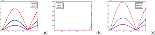
. In these figures, one can observe that a sufficient amount of mesh points and computed solutions are in the boundary layer region. we call that, the boundary layer resolving property of the scheme. In and , the absolute error of the three schemes are depicted for different mesh numbers
and
. As the mesh numbers increases, the accuracy of the schemes increases. In , the effect of the delay parameter
on the solution and the influence of
on the thickness of the boundary layer are shown. As the magnitude of the delay parameter increase, the thickness of the boundary layer increases.
Figure 1. Effect of the delay parameter on solution: (a) Example 4.1 and (b) Example 4.2 for
.
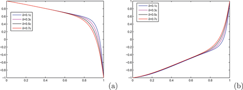
Figure 2. Formation of the boundary layer as goes small in (a) Example 4.1 in (b) Example 4.2.
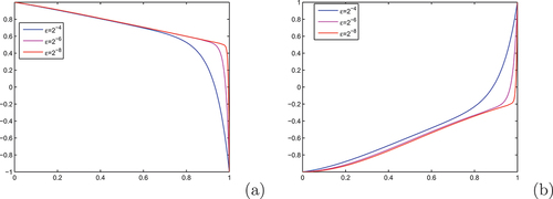
Figure 3. Example 4.1, Layer resolving property of the schemes for : on (a) Scheme I, on (b) Scheme III for
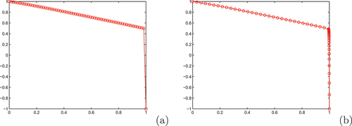
Figure 4. Layer resolving property of the schemes for Example 4.2: in (a) Scheme I, in (b) Scheme III for
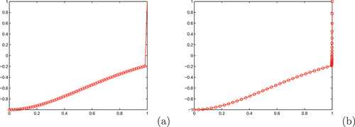
Figure 5. Example 4.1, absolute error of the schemes for different mesh numbers on (a) Scheme I, on (b) Scheme II and on (c) Scheme III for
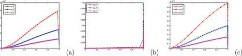
Figure 6. Example 4.2, absolute error of the schemes for different mesh numbers on (a) Scheme I, on (b) Scheme II and on (c) Scheme III for
In , the maximum absolute error, -uniform error and
-uniform rate of convergence of Example 4.1 and 4.2 are given for the Scheme II. Similarly, in Tables, 2 and 6, the maximum absolute error,
-uniform error, and the
-uniform rate of convergence of Scheme III are given. As one can see from the results in these tables, Scheme II has inferior accuracy and rate of convergence to Scheme III. The results in , show that the schemes are uniformly convergent(converges independent of the perturbation parameter as the perturbation parameter goes small) with an order of convergence one. In , the maximum absolute error of Scheme III for different values of the delay parameter is given. As is seen in these tables, the scheme converges independently of the delay parameter. In , one can see the comparison of Scheme III with the results in (Kadalbajoo & Ramesh, Citation2007; Kumar & Kadalbajoo, Citation2012), and (Woldaregay & Duressa, Citation2021a). We confirm that the proposed Scheme III is more accurate than the results in (Kadalbajoo & Ramesh, Citation2007; Kumar & Kadalbajoo, Citation2012), and (Woldaregay & Duressa, Citation2021a).
Table 1. Example 4.1, maximum absolute error of Scheme II in (27) for
Table 2. Example 4.1, maximum absolute error of Scheme III in (30) for
Table 3. Example 4.1, maximum absolute error of Scheme III in (30) for different values of with
Table 4. Example 4.1, comparison of maximum absolute error of Scheme III in (30) with results in (Kadalbajoo & Ramesh, Citation2007; Kumar & Kadalbajoo, Citation2012) and (Woldaregay & Duressa, Citation2021a)
Table 5. Example 4.2, maximum absolute error of Scheme II in (27) for for
Table 6. Example 4.2, maximum absolute error of Scheme III in (30) for
Table 7. Example 4.2, maximum absolute error of Scheme III in (30) for different values of with
5. Conclusion
In this paper, three numerical schemes are developed and investigated for solving singularly perturbed DDEs. Solution of the considered equation exhibits boundary layer. The developed numerical schemes: Scheme I (non-standard mid-point upwind FDM on uniform mesh), Scheme II (standard mid-point upwind FDM on Shishkin mesh), and Scheme III (non-standard mid-point upwind FDM on Shishkin mesh). The stability of the schemes is investigated using the construction of a barrier function for the solution bound. Uniform convergence of the schemes is stated and proved. The applicability of the schemes is investigated by considering two test examples for different mesh sizes and parameter values. The effect of the perturbation parameter and the delay parameter on the solution is shown using figures and tables. The proposed Scheme III is layer resolving and uniformly convergent with an order of convergence one. It gives more accurate numerical results than Scheme II. Scheme III can be extendible for solving higher dimensional singularly perturbed problems. In future works, we extend Scheme III for semi-linear and higher dimensional singularly perturbed problems.
Acknowledgements
I would like to thank the editor and anonymous referees for careful reading and giving fruitful comments for improving the quality and content of the manuscript.
Disclosure statement
No potential conflict of interest was reported by the author(s).
Additional information
Funding
Notes on contributors
Mesfin Mekuria Woldaregay
Mesfin Mekuria Woldaregay received his Ph.D. in Mathematics from Jimma University in 2021. Currently, he is working at Adama Science and Technology University, Department of Applied Mathematics as a researcher and lecturer. His research interests span the areas of numerical solution of differential equations, focusing on singularly perturbed problems. He has published more than 25 research articles in reputable journals. He also made numerous contributions in serving as a reviewer, and he is currently serving as an associate editor for the Ethiopian journal of sciences and sustainable development. So far, he has supervised four MSc students to completion and currently supervising four MSc students.
References
- Baker, C. T. H., Bocharov, G. A., & Rihan, F. A., A report on the use of delay differential equations in numerical modeling in the biosciences, Citeseer, 1999.
- Bellen, A., & Zennaro, M. (2003). Numerical methods for delay differential equations. Clarendon Press.
- Bushnaq, S., Shah, K., Tahir, S., Ansari, K. J., Sarwar, M., & Abdeljawad, T. (2022). Computation of numerical solutions to variable order fractional differential equations by using non-orthogonal basis. AIMS Mathematics, 7(6), 10917–13. https://doi.org/10.3934/math.2022610
- Elsheikh, S., Ouifki, R., & Patidar, K. C. (2014). A non-standard finite difference method to solve a model of HIV–Malaria co-infection. Journal of Difference Equations and Applications, 20(3), 354–378. https://doi.org/10.1080/10236198.2013.821116
- He, X., & Wang, K. (2018). New finite difference methods for singularly perturbed convection-diffusion equations. Taiwanese Journal of Mathematics, 22(4), 949–978. https://doi.org/10.11650/tjm/171002
- Izadi, M., Yüzbaşı, S., & Ansari, K. J. (2021). Application of Vieta–Lucas series to solve a class of multi-pantograph delay differential equations with singularity. Symmetry, 13(12), 2370. https://doi.org/10.3390/sym13122370
- Kadalbajoo, M. K., Patidar, K. C., & Sharma, K. K. (2006). ε-uniformly convergent fitted methods for the numerical solution of the problems arising from singularly perturbed general DDEs. Applied Mathematics and Computation, 182(1), 119–139. https://doi.org/10.1016/j.amc.2006.03.043
- Kadalbajoo, M. K., & Ramesh, V. P. (2007). Numerical methods on Shishkin mesh for singularly perturbed delay differential equations with a grid adaptation strategy. Applied Mathematics and Computation, 188(2), 1816–1831. https://doi.org/10.1016/j.amc.2006.11.046
- Kellogg, T., & Tsan, A. (1978). Analysis of some difference approximations for a singular perturbation problem without turning point. Mathematics of Computation, 32(144), 1025–1039. https://doi.org/10.1090/S0025-5718-1978-0483484-9
- Kuang, Y. (1993). Delay differential equations: With applications in population dynamics. Academic Press.
- Kumar, D., & Kadalbajoo, M. K. (2012). Numerical treatment of singularly perturbed delay differential equations using B-Spline collocation method on Shishkin mesh. Jnaiam, 7(3–4), 73–90.
- Lopez, A. G. (2020). On an electrodynamic origin of quantum fluctuations. Nonlinear Dynamics, 102(1), 621–634. https://doi.org/10.1007/s11071-020-05928-5
- Mahaffy, P. R., A’Hearn, M. F., Atreya, S. K., Bar-Nun, A., Bruston, P., Cabane, M., Carignan, G. R., Coll, P., Crifo, J. F., Ehrenfreund, P., Harpold, D., Gorevan, S., Israel, G., Kasprzak, W., Mumma, M. J., Niemann, H. B., Owen, T., Raulin, F., Riedler, W., … Strazzulla, G. (1999). The Champollion cometary molecular analysis experiment. Advances in Space Research, 23(2), 349–359. https://doi.org/10.1016/S0273-1177(99)00056-3
- Makroglou, A., Li, J., & Kuang, Y. (2006). Mathematical models and software tools for the glucose-insulin regulatory system and diabetes: An overview. Applied Numerical Mathematics, 56(3–4), 559–573. https://doi.org/10.1016/j.apnum.2005.04.023
- Mickens, R. E. (2002). Non-standard finite difference schemes for differential equations. Journal of Difference Equations and Applications, 8(9), 823–847. https://doi.org/10.1080/1023619021000000807
- Mickens, R. E. (2005). Advances in the applications of Non-standard finite difference schemes. World Scientific.
- Miller, J. J., O’Riordan, E., & Shishkin, G. I. (2012). Fitted numerical methods for singular perturbation problems: Error estimates in the maximum norm for linear problems in one and two dimensions. World Scientific.
- Patidar, K. C. (2005). On the use of non-standard finite difference methods. Journal of Difference Equations and Applications, 11(8), 735–758. https://doi.org/10.1080/10236190500127471
- Patidar, K. C. (2008). A robust fitted operator finite difference method for a two-parameter singular perturbation problem 1. Journal of Difference Equations and Applications, 14(12), 1197–1214. https://doi.org/10.1080/10236190701817383
- Patidar, K. C. (2016). Non-standard finite difference methods: Recent trends and further developments. Journal of Difference Equations and Applications, 22(6), 817–849. https://doi.org/10.1080/10236198.2016.1144748
- Roos, H. G., Stynes, M., & Tobiska, L. R. (2008). Numerical methods for singularly perturbed differential equations. Springer Science & Business Media.
- Salpeter, E. E., & Salpeter, S. R. (1998). Mathematical model for the epidemiology of tuberculosis, with estimates of the reproductive number and infection-delay function. American Journal of Epidemiology, 147(4), 398–406. https://doi.org/10.1093/oxfordjournals.aje.a009463
- Shah, K., Arfan, M., Ullah, A., Al-Mdallal, Q., Ansari, K. J., & Abdeljawad, T. (2022). Computational study on the dynamics of fractional order differential equations with applications. Chaos, Solitons, and Fractals, 157, 111955. https://doi.org/10.1016/j.chaos.2022.111955
- Sitthiwirattham, T., Gul, R., Shah, K., Mahariq, I., Soontharanon, J., Khursheed, K., & Ansari, K. J. (2021). Study of implicit-impulsive differential equations involving Caputo-Fabrizio fractional derivative. AIMS Mathematics, 7(3), 4017–4037. https://doi.org/10.3934/math.2022222
- Tian, H. (2002). The exponential asymptotic stability of singularly perturbed delay differential equations with a bounded lag. Journal of Mathematical Analysis and Applications, 270(1), 143–149. https://doi.org/10.1016/S0022-247X(02)00056-2
- Usta, F., Akyiğit, M., Say, F., & Ansari, K. J. (2022). Bernstein operator method for approximate solution of singularly perturbed Volterra integral equations. Journal of Mathematical Analysis and Applications, 507(2), 125828. https://doi.org/10.1016/j.jmaa.2021.125828
- Woldaregay, M. M., & Duressa, G. F. (2021a). Robust mid-point upwind scheme for singularly perturbed delay differential equations. Computational and Applied Mathematics, 40(5), 1–12. https://doi.org/10.1007/s40314-021-01569-5
- Woldaregay, M. M., & Duressa, G. F. (2021b). Robust numerical scheme for solving singularly perturbed differential equations involving small delays. Applied Mathematics E-Notes, 21, 622–633. http://www.math.nthu.edu.tw/amen/