Actuarial measures, aggregate loss models, and insurance applications of the sine exponentiated Burr XII distribution

ABSTRACT

The appropriate use of trigonometric functions in distribution theory can not be over-emphasized. In this paper, an extension of the exponentiated Burr XII distribution is proposed via the sine-Gfamily of distributions. This distribution is known as the sine exponentiated Burr XII distribution. The density is decreasing and right skewed with varying degree of peakedness whereas the hazard rate is decreasing and unimodal shaped. Mathematical properties such as the quantile function, moments, incomplete moments, moment generating function, and order statistics are derived. Also, actuarial measures such as value at risk, tail value at risk, and tail variance are derived and studied. The results show that the actuarial measures of the SEBXII distribution increase with increasing confidence level an indication that the SEBXII distribution is heavy-tailed. Under collective risk model, the mean and variance of the aggregate loss distribution where the frequency distribution for the claim count is Poisson are derived and studied. Estimates of the expected payout and the variance of the payout for the aggregate loss are obtained for varying parameter values. Five estimation approaches are used namely the maximum likelihood, least squares, weighted least squares, percentile, and Anderson-Darling are employed in examining the behavior of the proposed distribution. Simulations are carried for each of the estimation method. The results show that in most of the estimation methods, the AB and MSE approaches zero as the sample size increases, an indication that the estimators are consistent. That is the estimators of the proposed distribution are consistent for all the estimation methods. The usefulness of the proposed distribution is demonstrated with two insurance loss datasets. The results show that the proposed distribution provide the best parametric fit for the two datasets. The proposed distribution is flexible and capable of modeling heavy-tailed datasets.

KEYWORDS:

• Exponentiated Burr XII
• insurance loss data
• aggregate loss
• actuarial measures
• Sine-G family
• heavy-tailed distributions

1. Introduction

The modeling of random processes that are often observed in applied sciences remain a growing concern for researchers to investigate. Some researchers have proposed many families of distributions in the literature in an attempt to improve the flexibility of existing distributions. For example see Zografos and Balakrishman (2009); Eugene et al. (2002); Gupta and Kundu (2001); Cordeiro and de Castro (2011).

New distributions based on trigonometric functions are gaining popularity. These distributions are mostly flexible by making use of trigonometric functions curvature properties. Without changing any existing parameters, additional power is particularly acquired in the tails of the distribution (Chesneau & Artault, 2021; Chesneau & Jamal, 2019; Chesneau et al., 2019; Jamal et al., 2021; Mahmood et al., 2019; Souza et al., 2019). Trigonometric functions have several uses in many fields, including mathematics, engineering, medicine, and finance. Gilbert (1895) first used the sine distribution to calculate the impact angles that meteorites had on the moon’s craters.

The sine-G family of distributions was introduced by Souza (2015). Let F(x) be the cumulative distribution function (CDF) and f(x) be the probability density function (PDF). Then, if a random variable X follows the sine-G family of distributions, its CDF is designated by

(1) $\begin{array}{l}\mathit{F}(\mathit{x})=\mathit{sin}(\frac{\pi }{2}\mathit{G}(\mathit{x})),\mathit{x}\in \mathbb{R},\end{array}$(1)

with corresponding PDF given by

(2) $\begin{array}{l}\mathit{f}(\mathit{x})=\frac{\pi }{2}\mathit{g}(\mathit{x})\mathit{cos}(\frac{\pi }{2}\mathit{G}(\mathit{x})),\mathit{x}\in \mathbb{R}.\end{array}$(2)

It is desirable to know that the sine transformation can greatly increase the flexibility of F(x). This family of distributions has the advantages of being straightforward and having the same number of parameters for F(x) and G(x), preventing over-parameterization. As a result, F(x) can, by extension, increase G(x)’s flexibility. Similar works can be found in Famoyi et al. (2021); Isa et al. (2022); Abonongo et al. (2022); Abonongo et al. (2023); Souza (2015); Souza et al. (2019), and Chesneau and Jamal (2019).

The Burr system of distributions include 12 types of cumulative distribution functions that yields various density shapes (Burr, 1942, 1968, 1973; Burr & Cislak, 1968; Hatke, 1949; Rodriguez, 1977). Alizadeh et al. (2017) proposed and studied the Odd Burr power Lindley distribution. The attractiveness of this family of distributions for model fitting is that it combines a simple mathematical expression for cumulative distribution function with coverage in the skewness-kurtosis plane. The Burr XII distribution has received a lot of attention in modeling right skewed and heavty-tailed data. Some of the extensions of the Burr XII distribution can be found in Alizadeh et al. (2017); Cordeiro et al. (2018) and Gad et al. (2019). Kumar et al. (2017) introduced the exponentiated Burr XII (EBXII) distribution. Let G(x) be the CDF and g(x) be the PDF of the EBXII distribution. A random variable X, is said to follow the EBXII distribution if the CDF is given by

(3) $\begin{array}{l}\mathit{G}(\mathit{x})={(1-(1+{\mathit{x}}^{\mathit{\alpha }}{)}^{-\mathit{\theta }})}^{\mathit{\beta }},\mathit{x}>0,\mathit{\alpha }>0,\mathit{\beta }>0,\mathit{\theta }>0,\end{array}$(3)

where α, θ and β are shape parameters.

The PDF is given by

(4) $\begin{array}{l}\mathit{g}(\mathit{x})=\mathit{\alpha \beta \theta }{x}^{\mathit{\alpha }-1}(1+x^{\mathit{\alpha }}{)}^{-(\mathit{\theta }+1)}{(1-(1+{\mathit{x}}^{\mathit{\alpha }}{)}^{-\mathit{\theta }})}^{\mathit{\beta }-1},\mathit{x}>0,\end{array}$(4)

where α, θ and β are as defined earlier.

Additionally, due to the rigidity and unsatisfactory performance of the exponential, gamma, and Weibull distributions, Dutta and Perry (2006) disregarded them in their study on loss distributions. They concluded that one would need to use a model that is flexible enough. To develop flexible and useful distributions in the field of risk management, insurance, actuarial sciences, climate science, extreme value analysis, and portfolio optimization, it is essential to build on existing distributions or to develop new ones. In the literature, Ahmad et al. (2021) proposed a new exponential-X family of distributions with the new exponential Weibull (NE-Weibull) as a special distribution. Also, the new beta power transformed family of distributions with the new beta transformed Weibull model capable of modeling heavy-tailed dataset was proposed by Ahmad et al. (2022). The exponential T-X family of distributions was introduced by Ahmad et al. (2021). They proposed the exponential T-X Weibull (ETX-Weibull) model and study it properties with applications to insurance data. Nevertheless, Lone et al. (2023) examined the trade share dataset using a mixture of two log-Bilal distributions (MLBDs). Sindhu et al. (2023) proposed and studied a novel nonhomogeneous Poisson method on the basis of the new power function distribution. Also, Shafiq et al. (2023) proposed the unit Gumbel Type-II (UG-II) model and explored few statistical properties. The Shanker distribution was extended by Abushal et al. (2023) where they proposed the 2-component mixture of the Shanker model (2-CMSM). A significant feature of the 2-CMSM hazard rate function is that it has increasing, decreasing and upside down bathtub shapes.

Furthermore, from the literature, most existing distributions have a lot of parameters introduced so as to make them flexibility. This leads to computational difficulties and over-parameterization amongst others. Also, the EBXII distribution has not yet receive much attention in terms of enhancing its flexibility with the same number of parameters. This is an attempt to extend the EBXII distribution by the use of the sine function. In this vain, the main goal of this paper is to extend/improve the flexibility of the EBXII distribution without introducing additional parameter(s) via trigonometric functions. Therefore, the SEBXII is proposed and studied to enhance the flexibility and tail behavior of the EBXII distribution. The density of the SEBXII is decreasing and right skewed with varying degree of peakedness whereas the hazard rate is decreasing and unimodal shaped. With these desirable properties it is hoped that the SEBXII distribution will be a good candidate in modeling data. This distribution is a contribution on distributions based on trigonometric transformation. The density and hazard rate plots of the distribution are desirable. Also, the VaR, TVaR, and TV plots show that the SEBXII distribution is capable of modeling heavy tailed datasets. The usefulness of the proposed distribution is demonstrated with two insurance loss datasets.

The rest of the paper is organized as follows: Section 2 presents the SEBXII distribution. The mathematical properties of the distribution is presented in Section 3. The aggregate loss model is presented in Section 4. In Section 5, the estimation methods are presented. Monte Carlo simulations are carried out in Section 6. In Section 7, the applications of the SEBXII distribution is illustrated using two real-life datasets. The assumptions and limitations of the study are discussed in Section 8. Finally, the conclusion is presented in Section 9.

2. Sine exponentiated Burr XII distribution

In this section, the sine exponentiated Burr XII (SEBXII) distribution is proposed and studied. Considering Equation (3)(3) $\begin{array}{l}\mathit{G}(\mathit{x})={(1-(1+{\mathit{x}}^{\mathit{\alpha }}{)}^{-\mathit{\theta }})}^{\mathit{\beta }},\mathit{x}>0,\mathit{\alpha }>0,\mathit{\beta }>0,\mathit{\theta }>0,\end{array}$(3) as the baseline distribution in Equation (1)(1) $\begin{array}{l}\mathit{F}(\mathit{x})=\mathit{sin}(\frac{\pi }{2}\mathit{G}(\mathit{x})),\mathit{x}\in \mathbb{R},\end{array}$(1) , the SEBXII distribution is obtained with CDF given by

(5) $\begin{array}{ll}\mathit{F}(\mathit{x})=& \mathit{sin}\left[\frac{\pi }{2}{(1-{(1+{\mathit{x}}^{\mathit{\alpha }})}^{-\mathit{\theta }})}^{\mathit{\beta }}\right],\mathit{x}>0,\mathit{\alpha }>0,\\ & \mathit{\beta }>0,\mathit{\theta }>0,\end{array}$(5)

where α, θ and β are shape parameters.

Remark 1. When α = 1, one will obtain sine exponentiated Lomax (SELo) distribution-(New). When θ = 1, one will obtain sine exponentiated log-logistic (SELL) distribution-(New). Also, when β = 1, one will obtain the sine-Burr XII distribution (Isa et al., 2022).

The related PDF of the SEBXII distribution is given by

(6) $\begin{array}{l}\begin{array}{ll}\mathit{f}(\mathit{x})=& \frac{\mathit{\pi \alpha \beta \theta }}{2}{x}^{\mathit{\alpha }-1}(1+x^{\alpha }{)}^{-(\mathit{\theta }+1)}{(1-{(1+x^{\alpha })}^{-\mathit{\theta }})}^{\mathit{\beta }-1}\\ & \times \mathit{cos}[\frac{\pi }{2}{(1-{(1+x^{\alpha })}^{-\mathit{\theta }})}^{\mathit{\beta }}],\mathit{x}>0.\end{array}\end{array}$(6)

The corresponding hazard rate function is given by

(7) $\begin{array}{l}\mathit{h}(\mathit{x})=\frac{\begin{array}{l}\mathrm{\pi \alpha \beta \theta }{x}^{\mathit{\alpha }-1}(1+x^{\mathit{\alpha }}{)}^{-(\mathit{\theta }+1)}{(1-{(1+{\mathit{x}}^{\mathit{\alpha }})}^{-\mathit{\theta }})}^{\mathit{\beta }-1}\\ \times \mathit{cos}\left[\frac{\pi }{2}{(1-{(1+{\mathit{x}}^{\mathit{\alpha }})}^{-\mathit{\theta }})}^{\mathit{\beta }}\right]\end{array}}{2[1-\mathit{sin}\left[\frac{\pi }{2}{(1-{(1+{\mathit{x}}^{\mathit{\alpha }})}^{-\mathit{\theta }})}^{\mathit{\beta }}\right]]},\mathit{x}>0.\end{array}$(7)

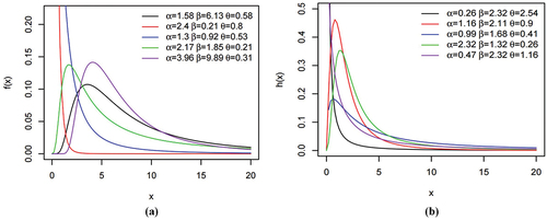
The plots for the density and hazard rate functions of the SEBXII distribution are shown in Figure 1. The density is decreasing and right skewed with varying degree of peakedness whereas the hazard rate is decreasing and unimodal shaped. This is a demonstration of the flexibility of the SEBXII distribution.

Figure 1. Plots for the density (a) and hazard rate (b) functions of the SEBXII distribution.

Before deriving the mathematical properties of the SEBXII distribution, it is desirable to obtain the linear representation of the PDF. Employing Taylor series expansion of the cosine function; $\mathit{cos}\mathit{x}=\sum _{\mathit{i}=0}^{\mathrm{\infty }}\frac{(-1{)}^{\mathit{i}}{x}^{2\mathit{i}}}{(2\mathit{i})!}$. Hence, from Equation (6)(6) $\begin{array}{l}\begin{array}{ll}\mathit{f}(\mathit{x})=& \frac{\mathit{\pi \alpha \beta \theta }}{2}{x}^{\mathit{\alpha }-1}(1+x^{\alpha }{)}^{-(\mathit{\theta }+1)}{(1-{(1+x^{\alpha })}^{-\mathit{\theta }})}^{\mathit{\beta }-1}\\ & \times \mathit{cos}[\frac{\pi }{2}{(1-{(1+x^{\alpha })}^{-\mathit{\theta }})}^{\mathit{\beta }}],\mathit{x}>0.\end{array}\end{array}$(6) ,

$\begin{array}{ll}\mathit{cos}\left[\frac{\pi }{2}{(1-{(1+{\mathit{x}}^{\mathit{\alpha }})}^{-\mathit{\theta }})}^{\mathit{\beta }}\right]=& \sum _{\mathit{i}=0}^{\mathrm{\infty }}\frac{(-1{)}^{\mathit{i}}(\mathit{\pi }/2{)}^{2\mathit{i}}}{2\mathit{i}}\\ & \times {(1-{(1+{\mathit{x}}^{\mathit{\alpha }})}^{-\mathit{\theta }})}^{2\mathit{i\beta }}.\end{array}$

This implies that

$\begin{array}{ll}\mathit{f}(\mathit{x})=& \mathit{\alpha \beta \theta }\sum _{\mathit{i}=0}^{\mathrm{\infty }}\frac{(-1{)}^{\mathit{i}}(\mathit{\pi }/2{)}^{2\mathit{i}}}{2\mathit{i}}{x}^{\mathit{\alpha }-1}(1+x^{\mathit{\alpha }}{)}^{-(\mathit{\theta }+1)}\\ & \times {(1-{(1+{\mathit{x}}^{\mathit{\alpha }})}^{-\mathit{\theta }})}^{2\mathit{i\beta }+\mathit{\beta }-1}.\end{array}$

Considering

$\begin{array}{ll}{(1-{(1+{\mathit{x}}^{\mathit{\alpha }})}^{-\mathit{\theta }})}^{2\mathit{i\beta }+\mathit{\beta }-1}=& \sum _{\mathit{j}=0}^{\mathrm{\infty }}(-1{)}^{\mathit{j}}(\genfrac{}{}{0ex}{}{2\mathit{i\beta }+\mathit{\beta }-1}{j})\\ & \times (1+x^{\mathit{\alpha }}{)}^{-\mathit{j\theta }},\end{array}$

the linear representation of the PDF of the SEBXII distribution becomes

(8) $\begin{array}{l}\mathit{f}(\mathit{x})=\mathit{\alpha \beta \theta }\sum _{\mathit{j}=0}^{\mathrm{\infty }}\sum _{\mathit{i}=0}^{\mathrm{\infty }}{\mathrm{\Phi }}_{\mathit{ij}}{x}^{\mathit{\alpha }-1}(1+x^{\mathit{\alpha }}{)}^{-\mathit{j\theta }-(\mathit{\theta }+1)},\end{array}$(8)

where ${\mathrm{\Phi }}_{\mathit{ij}}=\frac{(-1{)}^{\mathit{i}+\mathit{j}}(\mathit{\pi }/2{)}^{2\mathit{i}+1}}{2\mathit{i}!}(\genfrac{}{}{0ex}{}{2\mathit{i\beta }+\mathit{\beta }-1}{j})$.

3. Mathematical properties

In this section, some mathematical properties of the SEBXII distribution are derived.

3.1. Quantile function

The quantile function is used in obtaining random samples from a probability distribution. The quantile function of the SEBXII distribution is given by

$\begin{array}{l}{x}_{\mathit{p}}={[{(1-{(\frac{2}{\pi }\mathit{arcsin}(\mathit{p}))}^{1/\mathit{\beta }})}^{-1/\mathit{\theta }}-1]}^{1/\mathit{\alpha }},\mathit{p}\in (0,1).\end{array}$

3.2. Moments and incomplete moments

The moments are important in estimating measures of variation like the variance, standard deviation, coefficient of variation, mean deviation, median deviation, kurtosis, skewness amongst others.

The r^th non-central moment by definition is given by

$\begin{array}{l}{\mu }_{\mathit{r}}^{{}^{\prime }}={\int }_0^{\mathrm{\infty }}{x}^{\mathit{r}}\mathit{f}(\mathit{x})\mathit{dx}.\end{array}$

This implies

$\begin{array}{l}{\mu }_{\mathit{r}}^{{}^{\prime }}=\mathit{\alpha \beta \theta }\sum _{\mathit{j}=0}^{\mathrm{\infty }}\sum _{\mathit{i}=0}^{\mathrm{\infty }}{\mathrm{\Phi }}_{\mathit{ij}}{\int }_0^{\mathrm{\infty }}{x}^{\mathit{r}}{x}^{\mathit{\alpha }-1}(1+x^{\mathit{\alpha }}{)}^{-(\mathit{j\theta }+(\mathit{\theta }+1))}\mathit{dx}.\end{array}$

After some algebra, simplification and making use of the identity $\mathit{B}(\mathit{s},\mathit{t})={\int }_0^1{x}^{\mathit{s}-1}(1-\mathit{x}{)}^{\mathit{t}-1}\mathit{dx}$, one obtains

(9) $\begin{array}{l}{\mu }_r^{{}^{\mathit{\prime }}}=\mathit{\beta \theta }\sum _{\mathit{j}=0}^{\mathrm{\infty }}\sum _{\mathit{i}=0}^{\mathrm{\infty }}{\mathrm{\Phi }}_{\mathit{ij}}\mathit{B}(2+\frac{r}{\alpha }-\mathit{j\theta }-\mathit{\theta },1+\frac{r}{\alpha }),\mathit{\alpha }>\mathit{r},\end{array}$(9)

where $\mathit{B}(.,.)$ is the beta function with $\mathit{r}=1,2,3,\dots$

The values for the first four moments, standard deviation (σ), coefficient of variation (CV), coefficient of skewness (CS), and coefficient of kurtosis (CK) of the SEBXII distribution for four set of parameter values: I=(α = 1.82, β = 0.83, θ = 5.3), II=(α = 2.6, β = 0.14, θ = 1.82), III=(α = 1.1, β = 0.6, θ = 2.31), and IV=(α = 3.7, β = 0.31, θ = 4.52) are shown in Table 1 via numerical integration. The standard deviation (σ), coefficient of variation (CV), coefficient of skewness (CS), and coefficient of kurtosis (CK) are defined as $\mathit{\sigma }=\sqrt{{\mu }_2^{{}^{\prime }}-({\mu }_1^{{}^{\prime }}{)}^2}$, $\mathit{CV}=\frac{\sigma }{{\mu }_1^{{}^{\prime }}}$, $\mathit{CS}=\frac{{\mathit{\mu }}_3^{{}^{\prime }}-3{\mu }_1^{{}^{\prime }}{\mu }_2^{{}^{\prime }}+2({\mu }_1^{{}^{\prime }}{)}^3}{{\sigma }^3}$, and $\mathit{CK}=\frac{{\mathit{\mu }}_4^{{}^{\prime }}-4{\mu }_1^{{}^{\prime }}{\mu }_3^{{}^{\prime }}+6({\mu }_1^{{}^{\prime }}{)}^2{\mu }_2^{{}^{\prime }}-3({\mu }_1^{{}^{\prime }}{)}^4}{{\sigma }^4}$ respectively.

Table 1. First four moments, σ, CV, CS, and CK of the SEBXII distribution

${\mu }_{\mathit{r}}^{{}^{\prime }}$	I	II	III	IV
${\mu }_2^{{}^{\prime }}$	0.081	0.039	0.111	0.110
${\mu }_3^{{}^{\prime }}$	0.034	0.022	0.145	0.052
${\mu }_1^{{}^{\prime }}$	0.239	0.110	0.190	0.279
${\mu }_4^{{}^{\prime }}$	0.017	0.017	0.471	0.028
σ	0.155	0.164	0.274	0.179
CV	3.975	1.491	1.442	0.642
CS	7.862	2.673	4.640	0.587
CK	4.276	13.426	67.584	3.083

The r^th incomplete moment by definition is given by

(10) $\begin{array}{l}{M}_{\mathit{r}}(\mathit{x})={\int }_0^y{x}^{\mathit{r}}\mathit{f}(\mathit{x})\mathit{dx}.\end{array}$(10)

Substituting Equation (8)(8) $\begin{array}{l}\mathit{f}(\mathit{x})=\mathit{\alpha \beta \theta }\sum _{\mathit{j}=0}^{\mathrm{\infty }}\sum _{\mathit{i}=0}^{\mathrm{\infty }}{\mathrm{\Phi }}_{\mathit{ij}}{x}^{\mathit{\alpha }-1}(1+x^{\mathit{\alpha }}{)}^{-\mathit{j\theta }-(\mathit{\theta }+1)},\end{array}$(8) into Equation (10)(10) $\begin{array}{l}{M}_{\mathit{r}}(\mathit{x})={\int }_0^y{x}^{\mathit{r}}\mathit{f}(\mathit{x})\mathit{dx}.\end{array}$(10) , one obtains

$\begin{array}{l}{M}_{\mathit{r}}(\mathit{x})=\mathit{\alpha \beta \theta }\sum _{\mathit{j}=0}^{\mathrm{\infty }}\sum _{\mathit{i}=0}^{\mathrm{\infty }}{\mathrm{\Phi }}_{\mathit{ij}}{\int }_0^y{x}^{\mathit{r}}{x}^{\mathit{\alpha }-1}(1+x^{\mathit{\alpha }}{)}^{-(\mathit{j\theta }+(\mathit{\theta }+1))}\mathit{dx},\end{array}$

and solving, one obtains

$\begin{array}{l}{M}_{\mathit{r}}(\mathit{x})=\mathit{\beta \theta }\sum _{\mathit{j}=0}^{\mathrm{\infty }}\sum _{\mathit{i}=0}^{\mathrm{\infty }}{\mathrm{\Phi }}_{\mathit{ij}}\mathit{B}((1+x^{\mathit{\alpha }}{)}^{-1};2+\frac{r}{\alpha }-\mathit{j\theta }-\mathit{\theta },1+\frac{r}{\alpha }),\mathit{\alpha }>\mathit{r},\end{array}$

where $\mathit{B}(.;.,.)$ is the incomplete beta function with $\mathit{r}=1,2,3,\dots$

3.3. Moment generating function

The moment generating function (MGF) of a random variable X by definition is given as, $M_{\mathit{x}}(\mathit{t})=\mathbb{E}(e^{\mathit{tx}})$, if it exists. Using series expansion, $M_{\mathit{x}}(\mathit{t})=\sum _{\mathit{r}=0}^{\mathrm{\infty }}\frac{t^{\mathit{r}}}{\mathit{r}!}{\mu }_{\mathit{r}}^{{}^{\prime }}$. Thus,

$\begin{array}{l}{M}_{\mathit{x}}(\mathit{t})=\sum _{\mathit{r}=0}^{\mathrm{\infty }}\frac{t^{\mathit{r}}}{\mathit{r}!}\mathit{\beta \theta }\sum _{\mathit{j}=0}^{\mathrm{\infty }}\sum _{\mathit{i}=0}^{\mathrm{\infty }}{\mathrm{\Phi }}_{\mathit{ij}}\mathit{B}(2+\frac{r}{\alpha }-\mathit{j\theta }-\mathit{\theta },1+\frac{r}{\alpha }),\mathit{\alpha }>\mathit{r}.\end{array}$

Therefore, the MGF of the SEBXII distribution is given by

$\begin{array}{l}{M}_{\mathit{x}}(\mathit{t})=\frac{\mathit{\beta \theta }{\mathit{t}}^{\mathit{r}}}{\mathit{r}!}\sum _{\mathit{r}=0}^{\mathrm{\infty }}\sum _{\mathit{j}}^{\mathrm{\infty }}\sum _{\mathit{i}=0}^{\mathrm{\infty }}{\mathrm{\Phi }}_{\mathit{ij}}\mathit{B}(2+\frac{r}{\alpha }-\mathit{j\theta }-\mathit{\theta },1+\frac{r}{\alpha }),\mathit{\alpha }>\mathit{r}.\end{array}$

3.4. Actuarial measures

Actuarial measures such as value at risk (VaR), tail value at risk (TVaR), and tail variance (TV) of the SEBXII distribution are derived and studied.

3.4.1. Value at risk

The VaR is a benchmark for evaluating market risk. It is also called the quantile premium principle or quantile risk measure. It is usually expressed with a confidence level q (usually 90%, 95% or 99%), and represents the percentage of loss in portfolio value that will be equaled or exceeded only X percent of the time. The value at risk of the SEBXII distribution is given by

$\begin{array}{l}\mathit{VaR}(\mathit{x})={[{(1-{(\frac{2}{\pi }\mathit{arcsin}(\mathit{q}))}^{1/\mathit{\beta }})}^{-1/\mathit{\theta }}-1]}^{1/\mathit{\alpha }},\mathit{q}\in (0,1).\end{array}$

3.4.2. Tail value at risk

The TVaR is used in estimating the risk beyond a certain probability level. The TVaR of random variable X is defined as

(11) $\begin{array}{l}\mathit{TVaR}(\mathit{x})=\frac{1}{1-\mathit{q}}{\int }_{VaR}^{\mathrm{\infty }}\mathit{xf}(\mathit{x})\mathit{dx}.\end{array}$(11)

Substituting Equation (8)(8) $\begin{array}{l}\mathit{f}(\mathit{x})=\mathit{\alpha \beta \theta }\sum _{\mathit{j}=0}^{\mathrm{\infty }}\sum _{\mathit{i}=0}^{\mathrm{\infty }}{\mathrm{\Phi }}_{\mathit{ij}}{x}^{\mathit{\alpha }-1}(1+x^{\mathit{\alpha }}{)}^{-\mathit{j\theta }-(\mathit{\theta }+1)},\end{array}$(8) into Equation (11)(11) $\begin{array}{l}\mathit{TVaR}(\mathit{x})=\frac{1}{1-\mathit{q}}{\int }_{VaR}^{\mathrm{\infty }}\mathit{xf}(\mathit{x})\mathit{dx}.\end{array}$(11) will yield

$\begin{array}{l}\mathit{TVaR}(\mathit{x})=\frac{\mathit{\alpha \beta \theta }}{1-\mathit{q}}\sum _{\mathit{j}=0}^{\mathrm{\infty }}\sum _{\mathit{i}=0}^{\mathrm{\infty }}{\mathrm{\Phi }}_{\mathit{ij}}{\int }_{VaR}^{\mathrm{\infty }}\mathit{x}{x}^{\mathit{\alpha }-1}(1+x^{\alpha }{)}^{-\mathit{j\theta }-(\mathit{\theta }+1)}\mathit{dx}.\end{array}$

After some algebraic manipulations, one obtains the TVaR of the SEBXII distribution as

$\begin{array}{ll}\mathit{TVaR}(\mathit{x})=& \frac{\mathit{\beta \theta }}{1-\mathit{q}}\sum _{\mathit{j}=0}^{\mathrm{\infty }}\sum _{\mathit{i}=0}^{\mathrm{\infty }}{\mathrm{\Phi }}_{\mathit{ij}}\mathit{B}((1+\mathit{Va}{R}^{\mathit{\alpha }}{)}^{-1};\\ & 2+\frac{1}{\alpha }-\mathit{j\theta }-\mathit{\theta },1+\frac{1}{\alpha })\end{array}$

3.4.3. Tail variance

The TV is important in estimating the risk at the tails. By definition, the TV of a random variable X given by

$\begin{array}{l}\mathit{TV}(\mathit{x})=\mathbb{E}(X^2|\mathit{X}>x_{\mathit{q}})-(\mathit{TVaR}(\mathit{x}){)}^2.\end{array}$

Considering,

$\begin{array}{ll}\mathbb{E}(X^2|\mathit{X}>x_{\mathit{q}})=& \frac{\mathit{\alpha \beta \theta }}{1-\mathit{q}}\sum _{\mathit{j}=0}^{\mathrm{\infty }}\sum _{\mathit{i}=0}^{\mathrm{\infty }}{\mathrm{\Phi }}_{\mathit{ij}}\\ & {\int }_{VaR}^{\mathrm{\infty }}{x}^2{x}^{\mathit{\alpha }-1}(1+x^{\mathit{\alpha }}{)}^{-(\mathit{j\theta }+(\mathit{\theta }+1))}\mathit{dx}.\end{array}$

On solving,

$\begin{array}{ll}\mathit{TV}(\mathit{x})=& \frac{\mathit{\beta \theta }}{1-\mathit{q}}\sum _{\mathit{j}=0}^{\mathrm{\infty }}\sum _{\mathit{i}=0}^{\mathrm{\infty }}{\mathrm{\Phi }}_{\mathit{ij}}\mathit{B}((1+\mathit{Va}{R}^{\mathit{\alpha }}{)}^{-1};2+\frac{2}{\alpha }\\ & -\mathit{j\theta }-\mathit{\theta },1+\frac{2}{\alpha })-(\mathit{TVaR}(\mathit{x}){)}^2.\end{array}$

Table 2 shows the simulation results for the actuarial measures for n = 200 and different set of parameter values. The results show that the actuarial measures of the SEBXII distribution increase with increasing confidence level an indication that the SEBXII distribution is leptokurtic and heavy-tailed. This is confirmed by the plots in Figures 2-4 where the plots are all increasing at varying parameter values for VaR, TVaR, and TV.

Figure 2. VaR plots for SEBXII distribution.

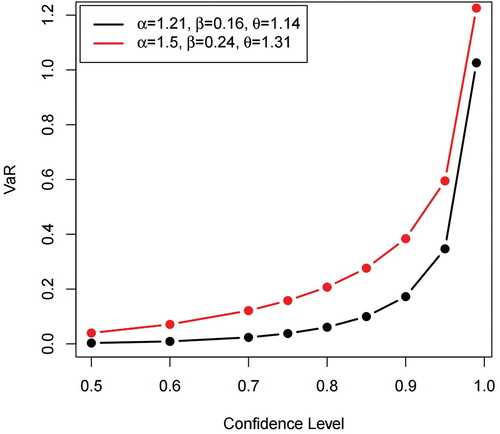
Figure 3. TVaR plots for SEBXII distribution.

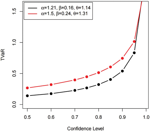
Figure 4. TV plots for SEBXII distribution.

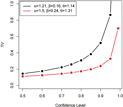
Table 2. Simulation results of actuarial measures for n = 200

Parameter value	Confidence level	VaR	TVaR	TV
	0.500	0.003	0.141	0.145
	0.600	0.009	0.175	0.176
	0.700	0.024	0.228	0.223
α = 1.21	0.750	0.038	0.267	0.258
β = 0.16	0.800	0.061	0.322	0.308
θ = 1.14	0.850	0.100	0.403	0.384
	0.900	0.173	0.539	0.521
	0.950	0.345	0.834	0.866
	0.990	1.026	1.907	2.762
	0.500	0.040	0.267	0.112
	0.600	0.071	0.320	0.125
	0.700	0.121	0.396	0.144
α = 1.5	0.750	0.158	0.447	0.157
β = 0.24	0.800	0.207	0.514	0.174
θ = 1.31	0.850	0.276	0.605	0.199
	0.900	0.384	0.745	0.239
	0.950	0.594	1.015	0.328
	0.990	1.226	1.829	0.670

The simulation steps are as follows:

1. Random sample of size n = 200 are generated from the SEBXII distribution and parameters estimated via maximum likelihood method.

2. 1000 repetitions are made to calculate the VaR, TVaR and TV for the SEBXII distribution.

3.5. Order statistics

Let $X_1,X_2,\dots ,X_{\mathit{n}}$ be a sample of size n from the SEBXII distribution and $X_{1:\mathit{n}}\le X_{2:\mathit{n}}\le \dots \le X_{\mathit{n}:\mathit{n}}$ denote the order statistics of the sample.

The PDF of the i^th order statistics is defined as

(12) $\begin{array}{l}{f}_{\mathit{i}:\mathit{n}}(\mathit{x})=\frac{\mathit{n}!}{(\mathit{i}-1)!(\mathit{n}-\mathit{i})!}\mathit{f}(\mathit{x})\sum _{\mathit{k}=0}^{\mathit{n}-\mathit{i}}(-1{)}^{\mathit{k}}(\genfrac{}{}{0ex}{}{\mathit{n}-\mathit{i}}{k})(\mathit{F}(\mathit{x}){)}^{\mathit{k}+\mathit{i}-1}.\end{array}$(12)

Substituting Equation (3)(3) $\begin{array}{l}\mathit{G}(\mathit{x})={(1-(1+{\mathit{x}}^{\mathit{\alpha }}{)}^{-\mathit{\theta }})}^{\mathit{\beta }},\mathit{x}>0,\mathit{\alpha }>0,\mathit{\beta }>0,\mathit{\theta }>0,\end{array}$(3) and Equation (4)(4) $\begin{array}{l}\mathit{g}(\mathit{x})=\mathit{\alpha \beta \theta }{x}^{\mathit{\alpha }-1}(1+x^{\mathit{\alpha }}{)}^{-(\mathit{\theta }+1)}{(1-(1+{\mathit{x}}^{\mathit{\alpha }}{)}^{-\mathit{\theta }})}^{\mathit{\beta }-1},\mathit{x}>0,\end{array}$(4) into Equation (12)(12) $\begin{array}{l}{f}_{\mathit{i}:\mathit{n}}(\mathit{x})=\frac{\mathit{n}!}{(\mathit{i}-1)!(\mathit{n}-\mathit{i})!}\mathit{f}(\mathit{x})\sum _{\mathit{k}=0}^{\mathit{n}-\mathit{i}}(-1{)}^{\mathit{k}}(\genfrac{}{}{0ex}{}{\mathit{n}-\mathit{i}}{k})(\mathit{F}(\mathit{x}){)}^{\mathit{k}+\mathit{i}-1}.\end{array}$(12) , will give

(13) $\begin{array}{ll}{f}_{\mathit{i}:\mathit{n}}(\mathit{x})=& \frac{\mathit{n}!\mathit{\alpha \beta \theta }}{2(\mathit{i}-1)!(\mathit{n}-\mathit{i})!}{x}^{\mathit{\alpha }-1}(1+x^{\mathit{\alpha }}{)}^{-(\mathit{\theta }+1)}\\ & \times {(1-(1+{\mathit{x}}^{\mathit{\alpha }}{)}^{-\mathit{\theta }})}^{\mathit{\beta }-1}\mathit{cos}\left[\frac{\pi }{2}{(1-{(1+{\mathit{x}}^{\mathit{\alpha }})}^{-\mathit{\theta }})}^{\mathit{\beta }}\right].\end{array}$(13)

The PDF of the n^th order statistics is defined as

(14) $\begin{array}{l}{f}_{\mathit{n}:\mathit{n}}(\mathit{x})=\mathit{n}[\mathit{F}(\mathit{x}){]}^{\mathit{n}-1}\mathit{f}(\mathit{x}).\end{array}$(14)

Substituting Equation (3)(3) $\begin{array}{l}\mathit{G}(\mathit{x})={(1-(1+{\mathit{x}}^{\mathit{\alpha }}{)}^{-\mathit{\theta }})}^{\mathit{\beta }},\mathit{x}>0,\mathit{\alpha }>0,\mathit{\beta }>0,\mathit{\theta }>0,\end{array}$(3) and Equation (4)(4) $\begin{array}{l}\mathit{g}(\mathit{x})=\mathit{\alpha \beta \theta }{x}^{\mathit{\alpha }-1}(1+x^{\mathit{\alpha }}{)}^{-(\mathit{\theta }+1)}{(1-(1+{\mathit{x}}^{\mathit{\alpha }}{)}^{-\mathit{\theta }})}^{\mathit{\beta }-1},\mathit{x}>0,\end{array}$(4) into Equation (14)(14) $\begin{array}{l}{f}_{\mathit{n}:\mathit{n}}(\mathit{x})=\mathit{n}[\mathit{F}(\mathit{x}){]}^{\mathit{n}-1}\mathit{f}(\mathit{x}).\end{array}$(14) , the PDF of the n^th order statistics becomes

(15) $\begin{array}{ll}{f}_{\mathit{n}:\mathit{n}}(\mathit{x})=& \frac{\mathit{n\pi \alpha \beta \theta }}{2}{x}^{\mathit{\alpha }-1}(1+x^{\mathit{\alpha }}{)}^{-(\mathit{\theta }+1)}{(1-(1+{\mathit{x}}^{\mathit{\alpha }}{)}^{-\mathit{\theta }})}^{\mathit{\beta }-1}\\ & \times \mathit{cos}\left[\frac{\pi }{2}{(1-{(1+{\mathit{x}}^{\mathit{\alpha }})}^{-\mathit{\theta }})}^{\mathit{\beta }}\right]\\ & \times \mathit{sin}{\left[\frac{\pi }{2}{(1-{(1+{\mathit{x}}^{\mathit{\alpha }})}^{-\mathit{\theta }})}^{\mathit{\beta }}\right]}^{\mathit{n}-1}.\end{array}$(15)

The PDF of the first order statistics is given by

(16) $\begin{array}{l}{f}_{1:\mathit{n}}(\mathit{x})=\mathit{n}[1-\mathit{F}(\mathit{x}){]}^{\mathit{n}-1}\mathit{f}(\mathit{x}).\end{array}$(16)

Substituting Equation (3)(3) $\begin{array}{l}\mathit{G}(\mathit{x})={(1-(1+{\mathit{x}}^{\mathit{\alpha }}{)}^{-\mathit{\theta }})}^{\mathit{\beta }},\mathit{x}>0,\mathit{\alpha }>0,\mathit{\beta }>0,\mathit{\theta }>0,\end{array}$(3) and Equation (4)(4) $\begin{array}{l}\mathit{g}(\mathit{x})=\mathit{\alpha \beta \theta }{x}^{\mathit{\alpha }-1}(1+x^{\mathit{\alpha }}{)}^{-(\mathit{\theta }+1)}{(1-(1+{\mathit{x}}^{\mathit{\alpha }}{)}^{-\mathit{\theta }})}^{\mathit{\beta }-1},\mathit{x}>0,\end{array}$(4) into Equation (16)(16) $\begin{array}{l}{f}_{1:\mathit{n}}(\mathit{x})=\mathit{n}[1-\mathit{F}(\mathit{x}){]}^{\mathit{n}-1}\mathit{f}(\mathit{x}).\end{array}$(16) , the PDF of the first order statistics becomes

(17) $\begin{array}{ll}{f}_{1:\mathit{n}}(\mathit{x})=& \frac{\mathit{n\pi \alpha \beta \theta }}{2}{x}^{\mathit{\alpha }-1}(1+x^{\mathit{\alpha }}{)}^{-(\mathit{\theta }+1)}{(1-(1+{\mathit{x}}^{\mathit{\alpha }}{)}^{-\mathit{\theta }})}^{\mathit{\beta }-1}\\ & \times \mathit{cos}\left[\frac{\pi }{2}{(1-{(1+{\mathit{x}}^{\mathit{\alpha }})}^{-\mathit{\theta }})}^{\mathit{\beta }}\right]\\ & \times {[1-\sin \left[\frac{\pi }{2}{(1-{(1+{\mathit{x}}^{\mathit{\alpha }})}^{-\mathit{\theta }})}^{\mathit{\beta }}\right]]}^{\mathit{n}-1}.\end{array}$(17)

4. Aggregate loss models under collective risk theory

In this section, the aggregate loss models of the SEBXII distribution are presented. Suppose N claims are experienced in the past and each unit x_i is the claim size which is independent identical distributed SEBXII with parameter α, β, and θ. The aggregate loss S is defined as $\mathit{S}=x_1+x_2+x_3+\dots +x_{\mathit{N}}$. If the individual loss amounts x_i are independent on the annual loss frequency N, then the PDF of the aggregate loss is defined as

$\begin{array}{l}{f}_{\mathit{s}}(\mathit{s})=\sum _{\mathit{i}=1}^{\mathrm{\infty }}\mathit{Pr}(\mathit{N}=\mathit{i})f_x^{\ast i}(\mathit{s}),\end{array}$

where $f_x^{\ast i}(\mathit{s})$ is the i^th fold convolution of S. The mean and variance of the aggregate loss distribution are defined as

$\begin{array}{l}\mathit{E}(\mathit{S})=\mathbb{E}(\mathit{N})\mathbb{E}(\mathit{X})\end{array}$

and

$\begin{array}{l}\mathit{V}(\mathit{S})=\mathbb{E}(\mathit{N})\mathit{V}(\mathit{X})+(\mathbb{E}(\mathit{X}){)}^2\mathit{V}(\mathit{N})\end{array}$

respectively.

Suppose the frequency of the loss follows the Poisson distribution with parameter λ, the mean and variance of the aggregate loss distribution can be written as

(18) $\begin{array}{l}\mathit{E}(\mathit{S})=\mathit{\lambda \beta \theta }\sum _{\mathit{j}=0}^{\mathrm{\infty }}\sum _{\mathit{i}=0}^{2\mathit{i}}{\mathrm{\Phi }}_{\mathit{ij}}\mathit{B}(2+\frac{1}{\alpha }-\mathit{j\theta }-\mathit{\theta },1+\frac{1}{\alpha })\end{array}$(18)

and

(19) $\begin{array}{l}\mathit{V}(\mathit{S})=\mathit{\lambda \beta \theta }\sum _{\mathit{j}=0}^{\mathrm{\infty }}\sum _{\mathit{i}=0}^{2\mathit{i}}{\mathrm{\Phi }}_{\mathit{ij}}[\mathit{B}(2+\frac{2}{\alpha }-\mathit{j\theta }-\mathit{\theta },1+\frac{2}{\alpha })]\end{array}$(19)

respectively.

Making use of Equation (18)(18) $\begin{array}{l}\mathit{E}(\mathit{S})=\mathit{\lambda \beta \theta }\sum _{\mathit{j}=0}^{\mathrm{\infty }}\sum _{\mathit{i}=0}^{2\mathit{i}}{\mathrm{\Phi }}_{\mathit{ij}}\mathit{B}(2+\frac{1}{\alpha }-\mathit{j\theta }-\mathit{\theta },1+\frac{1}{\alpha })\end{array}$(18) and Equation (19)(19) $\begin{array}{l}\mathit{V}(\mathit{S})=\mathit{\lambda \beta \theta }\sum _{\mathit{j}=0}^{\mathrm{\infty }}\sum _{\mathit{i}=0}^{2\mathit{i}}{\mathrm{\Phi }}_{\mathit{ij}}[\mathit{B}(2+\frac{2}{\alpha }-\mathit{j\theta }-\mathit{\theta },1+\frac{2}{\alpha })]\end{array}$(19) the estimates of the mean (expected payout) and the variance of the payout for the aggregate loss are obtained. These are presented in Table 3.

Table 3. Mean and variance of aggregate loss of SEBXII under the Poisson distribution with λ = 5

Parameter value	$\mathbb{E}(\mathit{X})$	$\mathbb{E}(X^2)$	$\mathbb{E}(\mathit{S})$	V(S)
α = 1.52
β = 0.4	0.239	0.081	1.195	0.691
θ = 1.12
α = 2.6
β = 0.14	0.110	0.039	0.550	0.256
θ = 1.82
α = 1.1
β = 0.4	0.190	0.111	0.950	0.739
θ = 0.6
α = 3.7
β = 0.31	0.279	0.110	1.395	0.939
θ = 4.52

5. Estimation methods

In this section, five methods of estimation are presented on how to obtain the parameters of the SEBXII distribution either by maximizing or minimizing the function under consideration. These are the maximum likelihood (MLE), least-squares (LS), weighted least-squares (WLS), percentile (PC), and Anderson-Darling (AD).

5.1. Maximum likelihood estimation

The maximum likelihood estimation (MLE) is obtained by maximizing the log-likelihood function. Let $x_1,x_2,\dots ,x_{\mathit{n}}$ be n random samples from the SEBXII distribution, then, the log-likelihood function which is a n × 1 parameter vector $\mathit{\Delta }=(\mathit{\alpha },\mathit{\beta },\mathit{\theta }{)}^{\mathit{T}}$ is given by

(20) $\begin{array}{ll}\mathit{\ell }(\mathit{\Delta })=& \mathit{n}(\mathit{log}\left(\frac{\mathit{\pi \alpha \beta \theta }}{2}\right))+(\mathit{\alpha }-1)\sum _{\mathit{i}=1}^{\mathit{n}}\mathit{log}(x_{\mathit{i}})-(\mathit{\theta }+1)\\ & \times \sum _{\mathit{i}=1}^{\mathit{n}}\mathit{log}(1+x_i^{\alpha })+(\mathit{\beta }-1)\sum _{\mathit{i}=1}^{\mathit{n}}\mathit{log}(1-(1+x_i^{\alpha }{)}^{-\mathit{\theta }})\\ & +\sum _{\mathit{i}=1}^{\mathit{n}}\mathit{log}(\mathit{cos}\left[\frac{\pi }{2}{(1-{(1+{\mathit{x}}^{\mathit{\alpha }})}^{-\mathit{\theta }})}^{\mathit{\beta }}\right]).\end{array}$(20)

Equating the score functions (differentiating Equation (20)(20) $\begin{array}{ll}\mathit{\ell }(\mathit{\Delta })=& \mathit{n}(\mathit{log}\left(\frac{\mathit{\pi \alpha \beta \theta }}{2}\right))+(\mathit{\alpha }-1)\sum _{\mathit{i}=1}^{\mathit{n}}\mathit{log}(x_{\mathit{i}})-(\mathit{\theta }+1)\\ & \times \sum _{\mathit{i}=1}^{\mathit{n}}\mathit{log}(1+x_i^{\alpha })+(\mathit{\beta }-1)\sum _{\mathit{i}=1}^{\mathit{n}}\mathit{log}(1-(1+x_i^{\alpha }{)}^{-\mathit{\theta }})\\ & +\sum _{\mathit{i}=1}^{\mathit{n}}\mathit{log}(\mathit{cos}\left[\frac{\pi }{2}{(1-{(1+{\mathit{x}}^{\mathit{\alpha }})}^{-\mathit{\theta }})}^{\mathit{\beta }}\right]).\end{array}$(20) with respect to each of the parameter) to zero and solving the resulting system of equations numerically, the maximum likelihood estimates of the parameters are obtained.

5.2. Method of Anderson-Darling

Let $x_1,x_2,\dots ,x_{\mathit{n}}$ be n random sample from the SEBXII distribution, the Anderson-Darling (AD) estimation is obtained by minimizing the following function:

(21) $\begin{array}{ll}\mathit{AD}(\mathit{\Delta })& =-\mathit{n}-\frac{1}{n}\sum _{1=1}^{\mathit{n}}(2\mathit{i}-1)[\mathit{log}\mathit{F}(x_{(\mathit{i})};\mathit{\alpha },\mathit{\beta },\mathit{\theta })\\ & +\mathit{log}\mathit{S}(x_{(\mathit{n}+1-\mathit{i})};\mathit{\alpha },\mathit{\beta },\mathit{\theta })]\\ & =-\mathit{n}-\frac{1}{n}[\mathit{log}(\mathit{sin}\left[\frac{\pi }{2}{(1-{(1+x_{(i)}^{\alpha })}^{-\mathit{\theta }})}^{\mathit{\beta }}\right])\\ & +\mathit{log}(1-\mathit{sin}\left[\frac{\pi }{2}{(1-{(1+x_{(n+1-i)}^{\alpha })}^{-\mathit{\theta }})}^{\mathit{\beta }}\right])].\end{array}$(21)

5.3. Method of percentile

Let $x_1,x_2,\dots ,x_{\mathit{n}}$ be n random sample from the SEBXII distribution, and $u_{\mathit{i}}=\mathit{i}/(\mathit{n}+1)$. The percentile (PC) estimation of the SEBXII distribution is obtained by minimizing the following function:

(22) $\begin{array}{l}\mathit{PC}(\mathit{\Delta })=\sum _{\mathit{i}=1}^{\mathit{n}}{[{\mathit{x}}_{\mathit{i}}-{[{(1-{(\frac{2}{\pi }\mathit{arcsin}(u_{\mathit{i}}))}^{1/\mathit{\beta }})}^{-1/\mathit{\theta }}-1]}^{1/\mathit{\alpha }}]}^2.\end{array}$(22)

5.4. Method of least square and weighted least square

Let $x_1,x_2,\dots ,x_{\mathit{n}}$ be n random sample from the SEBXII distribution, the least square (LS) estimation of the SEBXII is obtained by minimizing the following function:

(23) $\begin{array}{ll}\mathit{LS}(\mathit{\Delta })=& \sum _{\mathit{i}=1}^{\mathit{n}}{[\mathit{F}({\mathit{x}}_{(\mathit{i})},\mathit{\alpha },\mathit{\beta },\mathit{\theta })-\frac{i}{\mathit{n}+1}]}^2\end{array}$(23)

$\begin{array}{ll}=& \sum _{\mathit{i}=1}^n{[\sin \left[\frac{\pi }{2}{(1-{(1+x_{(i)}^{\alpha })}^{-\mathit{\theta }})}^{\mathit{\beta }}\right]-\frac{i}{\mathit{n}+1}]}^2.\end{array}$

The weighted least square (WLS) estimation of the parameters of the SEBXII distribution is obtained by minimizing the following function:

(24) $\begin{array}{ll}\mathit{WLS}(\mathit{\Delta })=& \sum _{\mathit{i}=1}^{\mathit{n}}\frac{(\mathit{n}+1{)}^2(\mathit{n}+2)}{\mathit{i}(\mathit{n}-\mathit{i}+1)}{[\mathit{F}({\mathit{x}}_{(\mathit{i})},\mathit{\alpha },\mathit{\beta },\mathit{\theta })-\frac{i}{\mathit{n}+1}]}^2\\ =& \sum _{\mathit{i}=1}^{\mathit{n}}\frac{(\mathit{n}+1{)}^2(\mathit{n}+2)}{\mathit{i}(\mathit{n}-\mathit{i}+1)}\\ & \times {[\sin \left[\frac{\pi }{2}{(1-{(1+x_{(i)}^{\alpha })}^{-\mathit{\theta }})}^{\mathit{\beta }}\right]-\frac{i}{\mathit{n}+1}]}^2.\end{array}$(24)

6. Monte Carlo simulation

In this section, simulation study to assess the performance of the five estimation methods is carried out. The nlminb function in the R program is used in the simulation. The function uses the L-BFGS-B optimization method. The simulation steps are as follows:

1. Generate N = 1000 sample of size $\mathit{n}=25,100,\$\text{break}\$200,350,500$ from the quantile function of the SEBXII distribution.

2. Compute the MLE, AD, LS, WLS, and PC parameter estimates of the sample obtained in (i).

3. For each parameter estimate, calculate the absolute baise (AB) and mean square error (MSE) defined as

   $\begin{array}{l}\mathit{AB}=\frac{1}{N}\sum _{\mathit{i}=1}^{\mathit{N}}({\hat{\Delta }}_{\mathit{i}}-{\Delta }_{\mathit{i}})\end{array}$

   and

   $\begin{array}{l}\mathit{MSE}=\frac{1}{N}\sum _{\mathit{i}=1}^{\mathit{N}}({\hat{\Delta }}_{\mathit{i}}-{\Delta }_{\mathit{i}}{)}^2\end{array}$

   for $\mathit{\Delta }=(\mathit{\alpha },\mathit{\beta },\mathit{\theta })$, respectively.

4. Steps (i) and (iii) are repeated for two sets of parameter values; $\mathit{I}=(\mathit{\alpha }=1.02,\mathit{\beta }=0.53,\mathit{\theta }=2.23)$ and $\mathit{II}=(\mathit{\alpha }=0.65,\mathit{\beta }=2.46,\mathit{\theta }=0.82)$.

Tables 4 and 5 show the simulation results of the five estimation methods. For most of the estimation methods, the AB and MSE approaches zero as the sample size increases, an indication that the estimators are consistent. Also, for smaller sample size, PC performed better for α and θ, while MLE performed better for β. For larger sample size, PC performed better for α, while MLE performed better for β and θ.

Table 4. Simulation results of AB and MSE for α = 1.02, β = 0.53, θ = 2.23

Parameter	n	MLE	AD	LS	WLS	PC
AB
	25	0.658	2.800	4.403	3.387	0.130
	100	0.245	2.200	2.199	3.215	0.019
α	200	0.155	1.948	1.188	3.170	0.019
	350	0.112	1.711	0.184	3.112	0.019
	500	0.098	1.568	0.118	3.103	0.019
	25	0.199	0.430	0.448	0.460	1.333
	100	0.110	0.419	0.446	0.456	0.759
β	200	0.082	0.445	0.446	0.454	0.602
	350	0.064	0.402	0.442	0.450	0.529
	500	0.057	0.396	0.440	0.444	0.402
	25	1.777	1.986	2.408	2.434	1.333
	100	0.420	1.985	2.094	2.199	0.759
θ	200	0.289	1.977	2.084	2.187	0.602
	350	0.203	1.960	2.062	2.206	0.529
	500	0.177	1.915	2.000	2.141	0.402
MSE
	25	1.112	8.346	3.383	12.315	0.169
	100	0.186	5.093	3.180	10.806	0.003
α	200	0.074	4.020	3.168	10.557	0.003
	350	0.034	3.102	3.164	10.451	0.003
	500	0.026	2.604	3.138	10.164	0.003
	25	0.057	0.185	0.200	0.211	0.086
	100	0.021	0.176	0.199	0.208	0.035
β	200	0.125	0.199	0.199	0.206	0.022
	350	0.008	0.162	0.198	0.202	0.017
	500	0.006	0.157	0.196	0.197	0.010
	25	1.267	7.141	8.743	5.543	1.777
	100	0.310	3.978	4.388	4.867	0.576
θ	200	0.138	3.952	4.348	4.835	0.362
	350	0.065	3.952	4.262	4.782	0.280
	500	0.051	3.915	4.060	4.604	0.161

Table 5. Simulation results of AB and MSE for α = 0.65, β = 2.46, θ = 0.82

Parameter	n	MLE	AD	LS	WLS	PC
AB
	25	0.885	7.818	10.786	12.441	0.351
	100	0.394	6.799	9.759	11.910	0.247
α	200	0.362	6.570	9.431	11.387	0.202
	350	0.356	6.422	9.251	11.222	0.180
	500	0.353	6.350	9.180	10.898	0.101
	25	0.991	2.207	2.204	2.290	1.652
	100	0.964	2.206	2.204	2.285	1.560
β	200	0.954	2.205	2.204	2.283	1.516
	350	0.953	2.205	2.203	2.276	1.477
	500	0.952	2.204	2.201	2.250	1.453
	25	0.435	0.817	0.818	0.819	0.408
	100	0.409	0.817	0.818	0.819	0.395
θ	200	0.400	0.817	0.818	0.819	0.387
	350	0.400	0.817	0.818	0.819	0.377
	500	0.398	0.816	0.818	0.703	0.350
MSE
	25	1.070	81.895	171.773	186.315	0.123
	100	0.172	48.552	108.399	145.148	0.115
α	200	0.134	44.069	94.093	131.182	0.100
	350	0.127	41.903	88.543	126.836	0.087
	500	0.125	40.890	85.974	119.217	0.022
	25	1.164	4.871	4.842	5.245	2.728
	100	0.979	4.866	4.857	5.225	2.434
β	200	0.932	4.859	4.856	5.211	2.297
	350	0.919	4.861	4.857	5.178	2.183
	500	0.914	4.856	4.842	5.066	2.112
	25	0.212	0.668	0.669	0.671	0.167
	100	0.172	0.668	0.669	0.671	0.150
θ	200	0.162	0.668	0.669	0.671	0.148
	350	0.160	0.668	0.665	0.671	0.142
	500	0.159	0.667	0.691	0.670	0.123

7. Applications

In this section, the usefulness and flexibility of the SEBXII distribution using insurance loss datasets are demonstrated. The performance of the SEBXII distribution is compared with the exponentiated Burr XII (Kumar et al., 2017), Burr XII (Burr, 1942), sine Burr XII (Isa et al., 2022), modified Weibull distribution (Sarhan & Zaindin, 2009), and flexible Lomax (Ijaz et al., 2020) distributions. The performance of the distributions about providing proper parametric fit to the dataset is compared using the Akaike information criterion (AIC), Bayesian information criterion (BIC), Cramér-von Misses ($W^{\ast }$), Anderson-Darling ($A^{\ast }$) and Kolmogorov Smirnov (K-S) statistics. The distribution with the least of these measures provide a reasonable fit to the dataset. The density function of exponentiated Burr XII (EBXII), Burr XII (BXII), sine Burr XII (SBXII), modified Weibull distribution (MWD), and flexible Lomax (FL) distributions are as follows:

$\begin{array}{ll}\mathit{f}(\mathit{x})=& \mathit{\alpha \beta \theta }{x}^{\mathit{\alpha }-1}(1+x^{\mathit{\alpha }}{)}^{-(\mathit{\theta }+1)}{(1-(1+{\mathit{x}}^{\mathit{\alpha }}{)}^{-\mathit{\theta }})}^{\mathit{\beta }-1},\\ & \mathit{x}>0,\mathit{\alpha },\mathit{\beta },\mathit{\theta }>0.\\ \mathit{f}(\mathit{x})=& \mathit{ck}{x}^{\mathit{c}-1}(1+x^{\mathit{c}}{)}^{-(\mathit{k}+1)},\mathit{x}>0,\mathit{c},\mathit{k}>0.\\ \mathit{f}(\mathit{x})=& \frac{\pi }{2}\frac{\mathit{ab}{\mathit{x}}^{\mathit{a}-1}}{(1+x^{\mathit{a}}{)}^{\mathit{b}+1}}\mathit{cos}\left(\frac{\pi }{2}(1-\frac{1}{(1+{\mathit{x}}^{\mathit{a}}{)}^{\mathit{b}}})\right),\\ & \mathit{x}>0,\mathit{a},\mathit{b}>0.\\ \mathit{f}(\mathit{x})=& (\mathit{\alpha }+\mathit{\beta \gamma }{x}^{\mathit{\gamma }-1})e^{-\mathit{\alpha x}-\mathit{\beta }{\mathit{x}}^{\mathit{\gamma }}},\mathit{x}>0,\mathit{\alpha },\mathit{\beta },\mathit{\gamma }>0.\\ \mathit{f}(\mathit{x})=& \frac{\mathit{ac}}{b^{\mathit{c}}}{x}^{\mathit{c}-1}{(1+{\left(\frac{x}{b}\right)}^{\mathit{c}})}^{-(\mathit{a}+1)},\mathit{x}>0,\mathit{a},\mathit{b},\mathit{c}>0.\end{array}$

7.1. Automobile collision data

The first dataset consist of severity; the average amount of claims (in pounds sterling) adjusted for inflation, of automobile collisions in the United Kingdom. It is available in the R package “insuranceData” (Wolny-Dominiak & Trzesiok, 2014).

The descriptive statistics of the automobile collision data as shown in Table 6 is evident that the data is heavy-tailed and right skewed. The box plot, histogram, violin plot, and kernel density plot of the data is shown in Figure 5. It confirms the results in Table 6. The hazard rate function of the automobile collision dataset is increasing since the curve is above the 45% degree line, this is shown in Figure 6.

Figure 5. Box plot, histogram, violin plot, and kernel density of the automobile collision data.

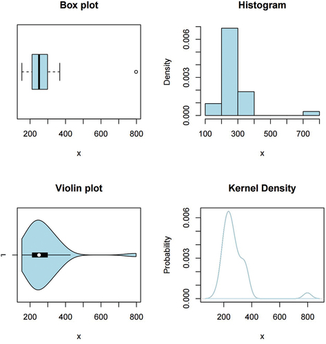
Figure 6. TTT plot of the automobile collision dataset.

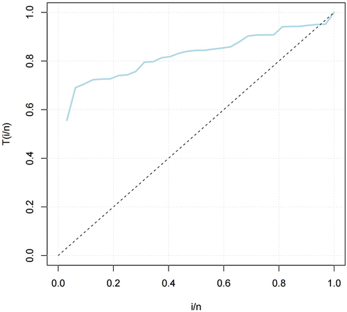
Table 6. Descriptive statistics of automobile collision data

No. of Claims	Mean	St. dev.	Kurtosis	Skewness	Minimum	Maximum
32	276.4	110.446	16.701	3.381	153.6	797.8

The MLEs, their standard errors (SEs) and the values of AIC, BIC, K-S, W*, and A* measures are shown in Table 7. The SEBXII distribution has the least of the information criteria and goodness-of-fit measures, and thus provides the best parametric fit to the automobile collision dataset compared to the other competing distributions.

Table 7. Mles, SEs, information criteria, goodness-of-fit measures for automobile collision data

Model		MLEs(SEs)	$-2\mathit{l}$	AIC	BIC	W*	A*	K-S(p-value)
	$\hat{\alpha }$	2.684 (0.626)
SEBXII	$\hat{\beta }$	2.948 (0.005)	360.253	366.253	370.650	0.039	0.311	0.080(0.776)
	$\hat{\theta }$	0.371 (0.086)
	$\hat{\alpha }$	2.033 (0.283)
EBXII	$\hat{\beta }$	3.516 (0.001)	419.262	425.262	429.659	0.077	0.861	0.451(0.582)
	$\hat{\theta }$	0.523 (0.073)
SBXII	$\hat{c}$	1.909 (5.781)	526.305	530.305	533.236	0.102	0.769	0.597(<0.002)
	$\hat{k}$	0.054 (0.165)
	$\hat{\alpha }$	0.004 (0.006)
MWD	$\hat{\beta }$	0.024 (0.009)	423.790	429.790	434.187	0.185	1.327	0.473(<0.004)
	$\hat{\gamma }$	−4.201 (0.002)
	$\hat{a}$	0.335 (0.187)
FL	$\hat{b}$	212.481 (16.524)	404.738	410.738	415.135	2.760	0.597	0.282(0.721)
	$\hat{c}$	11.967 (4.465)
BXII	$\hat{c}$	1.866 (5.328)	530.515	534.515	537.446	0.101	0.763	0.595(<0.002)
	$\hat{k}$	0.096 (0.275)

Figure 7 shows the empirical, fitted CDF and density of the SEBXII distribution for the automobile collision data. The plot shows that the SEBXII distribution provides a good parametric fit to the dataset.

Figure 7. Empirical, fitted CDF and density of the SEBXII distribution for automobile collision dataset.

7.2. Catastrophe data

The second dataset consist of the cost associated with catastrophe disaster in Australia from 1967 to 2014. The normed cost in millions of 2014 Australian dollars (AUD), computed as the inflated cost using consumer price index. This dataset is available in CASdatasets package (Dutang & Charpentier, 2020) of the R software. The descriptive statistics in Table 8 shows that the data is heavy-tailed and right skewed. Figure 8 shows the box plot, histogram, violin, and kernel density plot of the data which confirms the results in Table 8.

Figure 8. Box plot, histogram, violin plot, and kernel density of the catastrophe data.

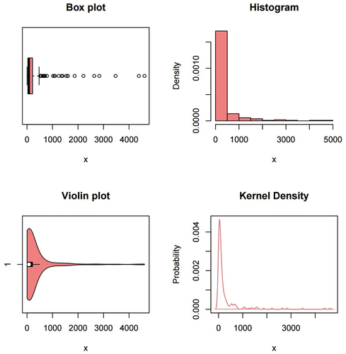
Table 8. Descriptive statistics of catastrophe data

No. of Claims	Mean	St. dev.	Kurtosis	Skewness	Minimum	Maximum
206	287.830	639.101	24.646	4.349	2.144	4605.932

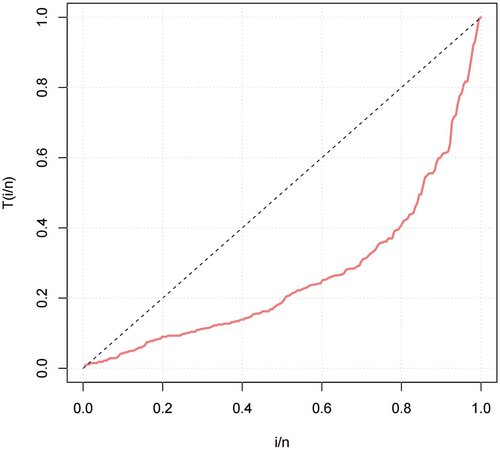
The hazard rate function of the catastrophe dataset is decreasing since the curve is convex below the 45% degree line, this is shown in Figure 9.

Figure 9. TTT plot of the catastrophe dataset.

The MLEs, their standard errors (SEs) and the values of AIC, BIC, K-S, p-value, W*, and A* measures are shown in Table 9. The SEBXII distribution has the least of the information criteria and goodness-of-fit measures, and thus provides the best parametric fit to the automobile the catastrophe dataset compared to the other competing distributions.

Table 9. Mles, SEs, information criteria, goodness-of-fit measures for catastrophe data

Model		MLEs(SEs)	$-2\mathit{l}$	AIC	BIC	W*	A*	K-S(P-value)
	$\hat{\alpha }$	0.282 (0.022)
SEBXII	$\hat{\beta }$	39.180 (0.004)	2587.485	2600.531	2610.515	0.116	0.491	0.118(0.802)
	$\hat{\theta }$	2.416 (0.123)
	$\hat{\alpha }$	0.308 (0.023)
EBXII	$\hat{\beta }$	72.710 (0.003)	2594.531	3118.389	3128.373	0.221	0.953	0.242(0.787)
	$\hat{\theta }$	2.999 (0.149)
SBXII	$\hat{c}$	5.229 (5.727)	2832.610	3158.249	3164.905	0.155	1.132	0.456(<0.002)
	$\hat{k}$	0.054 (0.165)
	$\hat{\alpha }$	−0.003 (0.006)
MWD	$\hat{\beta }$	0.035 (0.006)	2632.638	2639.370	2649.353	0.744	4.342	0.318(0.006)
	$\hat{\gamma }$	0.636 (0.041)
	$\hat{a}$	0.710 (0.176)
FL	$\hat{b}$	52.963 (15.943)	2589.851	3199.206	3209.189	0.136	1.014	0.209(0.582)
	$\hat{c}$	1.326 (0.163)
BXII	$\hat{c}$	6.239 (13.191)	2854.968	2858.968	2865.624	0.182	1.288	0.354(<0.002)
	$\hat{k}$	0.036 (0.076)

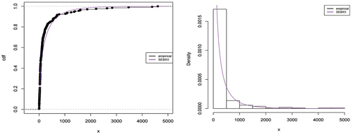
Figure 10 shows the empirical, fitted CDF and density of the SEBXII distribution for the catastrophe data. The plot shows that the SEBXII distribution provides a good parametric fit to the dataset.

Figure 10. Empirical, fitted CDF and density of the SEBXII distribution for catastrophe dataset.

8. Assumptions and limitations

In this paper, it is assumed that the EBXII distribution is a baseline distribution in the sine-G family of distributions. The limitations of this study has to do with choosing initial values to include in the simulations so as achieve convergence.

9. Conclusion

Recent studies have shown the potentials of trigonometric functions in proposing new distributions. This technique is flexible due to its desirable properties and mostly avoids over-parameterization. In this paper, an extension of the exponentiated Burr XII distribution is introduced via the sine-G family of distributions. This distribution is known as the sine exponentiated Burr XII distribution. The plots of the density can be decreasing and right skewed with varying degree of peakedness whereas the hazard rate plots can be decreasing and unimodal shaped. Mathematical properties such as the quantile function, moments, incomplete moments, moment generating function, and order statistics are derived. Actuarial measures such as value at risk, tail value at risk, and tail variance are derived and studied. The simulated results of the actuarial measures show that these measures increase with increasing confidence level an indication that the SEBXII distribution is heavy-tailed. Also, under collective risk model, the mean and variance of the aggregate loss distribution where the frequency distribution for the claim count is Poisson are derived and studied. Estimates of the expected payout and the variance of the payout for the aggregate loss are obtained for varying parameter values. To estimate the parameters of the SEBXII distribution, the following five different estimation approaches are used; maximum likelihood (MLE), least squares (LS), weighted least squares (WLS), percentile (PC), and Anderson-Darling (AD). The results of the Monte Carlo simulations show that the estimators of the SEBXII distribution are consistent under all the estimation methods. The usefulness of the SEBXII distribution is demonstrated with two insurance loss datasets namely; the automobile collision data and catastrophe data. The performance of the SEBXII distribution is compared with other competing distributions. It is evident that the SEBXII distribution provide the best parametric fit under the two datasets. This distribution is flexible and can be considered as a good candidate in modeling heavy-tailed datasets in insurance, finance, and other related fields.

Acknowledgements

The author wish to thank the editor and reviewers for their comments that helped in improving this paper.

Disclosure statement

No potential conflict of interest was reported by the author(s).

Funding

The author received no direct funding for this research.

Data availability statement

The data that support the findings of this study are available in the CASdatasets and insuranceData packages of the R software.

Additional information

Notes on contributors

John Abonongo

John Abonongo is a lecturer at the Department of Statistics and Actuarial Science, School of Mathematical Sciences, C. K. Tedam University of Technology and Applied Sciences, Navrongo, Ghana. He has published several research articles in several reputable journals. His research areas: Financial time series, distribution theory, stochastic theory, financial derivative and pricing, actuarial mathematics and Applications.

References

- Abonongo, J., Mwaniki, I. J., & Aduda, J. A. (2022). Sine F-Loss family of distribution: Properties and insurance applications. Applied Mathematics and Information Sciences, 16(5), 835–851.
- Abonongo, J., Mwaniki, I. J., & Aduda, J. A. (2023). A new family of F-Loss distributions: Properties and applications. Advances and Applications in Statistics, 87(1), 81–117. https://doi.org/10.17654/0972361723030
- Abushal, T. A., Sindhu, T. N., Lone, S. A., Hassan, M. K. H., & Shafiq, A. (2023). Mixture of Shanker distributions: Estimation, simulation, and application. Axiom, 12(3), 231. https://doi.org/10.3390/axioms12030231
- Ahmad, Z., Mahmoudi, E., Alizadeh, M., Roozegar, R., & Afify, A. Z. (2021). The exponential T-X family of distributions: Properties and an application to insurance data. Journal of Mathematics, 2021, 18. https://doi.org/10.1155/2021/3058170
- Ahmad, Z., Mahmoudi, E., Roozegar, R., Alizadeh, M., & Afify, A. Z. (2021). A new exponential X family: Modeling extreme value data in the finance sector. Mathematical Problems in Engineering, 2021, 14. https://doi.org/10.1155/2021/8759055
- Ahmad, Z., Mahoudi, E., & Alizadeh, M. (2022). Modeling insurance using a new beta power transformed family of distributions. Communications in Statistics-Simulations and Computation, 51(8), 4470–4491. https://doi.org/10.1080/03610918.2020.1743859
- Alizadeh, M., Altun, E., & Ozel, G. (2017). Odd burr power Lindley distribution with properties and applications. Gazi University Journal of Sciences, 30(3), 139–159.
- Burr, I. W. (1942). Cumulative frequency functions. The Annals of Mathematical Statistics, 13(2), 215–232. https://doi.org/10.1214/aoms/1177731607
- Burr, I. W. (1968). On a general system of distributions, iii. The sample range. Journal of the American Statistical Association, 63(322), 636–643. https://doi.org/10.1080/01621459.1968.11009282
- Burr, I. W. (1973). Parameters for a general system of distributions to match a grid of α 3 and α 4. Communications in Statistics, 2(1), 1–21. https://doi.org/10.1080/0361/0927/3088/27052
- Burr, I. W., & Cislak, P. J. (1968). On a general system of distributions: I. its curved-shaped characteristics, ii. The sample median. Journal of the American Statistical Association, 63(322), 627–635. https://doi.org/10.1080/01621459.1968.11009281
- Chesneau, C., & Artault, A. (2021). On a comparative study on some trigonometric classes of distributions by the analysis of practical datasets. Journal of Nonlinear Modelling Anal, 3(2), 225–262.
- Chesneau, C., Bakouch, H. S., & Hussain, T. (2019). A new class of probability distributions via cosine and sine functions with applications. Communications in Statistics - Simulation & Computation, 48(8), 2287–2300. https://doi.org/10.1080/03610918.2018.1440303
- Chesneau, C., & Jamal, F. (2019). The sine kumaraswamy-G family of distributions. HAL, hal-02120197.
- Cordeiro, G. M., & de Castro, M. (2011). A new family of generalized distribution. Journal of Statistical Computation and Simulation, 81(7), 883–898. https://doi.org/10.1080/00949650903530745
- Cordeiro, G. M., Yousof, H. M., Ramires, T. G., & Ortega, E. (2018). The burr XII system of densities: Properties, regression model and application. Journal of Statistical Computation and Simulation, 88(3), 432–456. https://doi.org/10.1080/00949655.2017.1392524
- Dutang, C., & Charpentier, A. (2020). Package CASdatasets.
- Dutta, K., & Perry, J. (2006). A tale of tails: An empirical analysis of loss distribution models for estimating operational risk capital. Tech. rep., Federal Reserve Bank of Boston, Working Paper No. 06-13.
- Eugene, N., Lee, C., & Famoye, F. (2002). The beta-normal distribution and its applications. Communications in Statistics-Theory and Methods, 31(4), 497–512. https://doi.org/10.1081/STA-120003130
- Famoyi, A., Algarni, A., & Almarashi, A. M. (2021). Sine inverse Lomax generated family of distributions with applications. Mathematical Problems in Engineering, 2021, 1–11. https://doi.org/10.1155/2021/1267420
- Gad, A. M., Hamedani, G. G., Salehabadi, S. M., & Yousof, H. M. (2019). The burr XII-Burr XII distribution: Mathematical properties and characterizations. Pakistan Journal of Statistics, 35(3), 229–248.
- Gilbert, G. K. (1895). The moon’s face; a study of the origin of its features. Bulletin of the Philosophical Society of Washington, 12, 241–249 doi:.
- Gupta, R. D., & Kundu, D. (2001). Generalized exponential distribution: Different method of estimations. Journal of Statistical Computation and Simulation, 69(4), 315–337. https://doi.org/10.1080/00949650108812098
- Hatke, M. A. (1949). A certain cumulative probability function. Annals of Mathematical Statistics, 20(3), 261–463. https://doi.org/10.1214/aoms/1177730002
- Ijaz, M., Asim, M., & Khali, A. (2020). Flexible Lomax Distribution. Songlanakarin Journal of Science and Technology, 42(5), 1125–1134.
- Isa, A. M., Ali, B., & Zannah, U. (2022). Sine Burr XII distribution: Properties and application to real data set. Arid Zone Journal of Basic and Applied Research, 1(3), 48–58. https://doi.org/10.55639/607lkji
- Jamal, F., Chesneau, C., & Aidi, K. (2021). The sine extended odd Fréchet-G family of distribution with applications to complete and censored data. Mathematica slovaca, 71(4), 961–982. https://doi.org/10.1515/ms-2021-0033
- Kumar, D., Saran, J., & Jain, N. (2017). The exponentiated burr XII distribution: Moments and estimation based on lower record values. Sri Lankan Journal of Applied Statistics, 18(1), 1–17. https://doi.org/10.4038/sljastats.v18i1.7930
- Lone, S. A., Sunhu, T. N., Anwar, S., Hassan, M. K. H., Alsahli, S. A., & Abushal, T. A. (2023). On construction and estimation of mixture of Log-Bilal distributions. Axioms, 12(3), 309. https://doi.org/10.3390/axioms12030309
- Mahmood, Z., Chesneau, C., & Tahir, M. H. (2019). A new sin-G family of distributions: Properties and applications. Bulletin of Computational Applied Mathematics, 7(1), 53–81.
- Rodriguez, N. (1977). A guide to the Burr type probability function. Biometrika, 64(1), 129–134. https://doi.org/10.1093/biomet/64.1.129
- Sarhan, A. M., & Zaindin, M. (2009). Modified Weibull distribution. Applied Sciences, 11(2009), 123–136.
- Shafiq, A., Sindhu, T. N., Hussain, Z., Mazucheli, J., & Alves, B. (2023). A flexible problem model for proportion data: Unit Gumbel type-II distribution, development, properties, different method of estimations and applications. Austrain Journal of Statistics, 52(2), 116–140. https://doi.org/10.17713/ajs.v52i2.1407
- Sindhu, T. N., Anwar, S., Hassan, M. K. H., Lone, S. A., Abushal, T. A., & Shafiq, A. (2023). An analysis of the new reliability model based on bathtub-shaped failure rate distribution with application to failure data. Mathematics, 11(4), 842. https://doi.org/10.3390/math11040842
- Souza, L. (2015). New Trigonometric Classes of Probabilistic Distributions. Ph.D. thesis,
- Souza, L., Junior, W. R. O., de Brito, C. C. R., Chesneau, C., Ferreira, T. A. E., & Soares, L. (2019). General properties for the cos-G class of distribution with applications. Eurasian Bulling Math, 2(2), 63–79.
- Wolny-Dominiak, A., & Trzesiok, M. (2014). Package insuranceData.
- Zografos, K., & Balakrishman, N. (2009). On families of beta and generalized gamma-generated distributions and associated inference. Statistical Methodology, 6(4), 344–362. https://doi.org/10.1016/j.stamet.2008.12.003