
 ?Mathematical formulae have been encoded as MathML and are displayed in this HTML version using MathJax in order to improve their display. Uncheck the box to turn MathJax off. This feature requires Javascript. Click on a formula to zoom.
ABSTRACT
In this paper, we study the inverse eigenvalue problem of constructing symmetric matrices whose graph is a tree, i.e. of constructing irreducible acyclic matrices from given eigendata consisting of the smallest and largest eigenvalues of their leading principal submatrices. We solve the problem completely for the case when the given eigenvalues are distinct and the subgraph of the tree induced by remains connected for
. The result generalizes the results known for matrices described by some specific trees. The proofs of the main results are constructive and so provide an algorithm for computing the actual entries of the required matrix. Numerical solutions of the problem are then obtained with SCILAB by feeding the eigendata and plugging in the adjacency matrix as inputs. We also make an attempt to find the number of solutions for several special families of unlabelled trees.
1. Introduction
An inverse eigenvalue problem (IEP) is the problem of reconstructing matrices of a pre-assigned structure which also satisfy the given constraints on eigenvalues and eigenvectors of the matrices or their submatrices. IEPs that require the construction of matrices having a pre-assigned pattern of zero entries are quite interesting. The pattern of zero entries of an symmetric matrix determines the structure of the underlying graph on n vertices. It has been seen that the structure of the underlying graph has a considerable influence on the spectrum of the corresponding matrix. For example, the smallest and the largest eigenvalues of a symmetric matrix whose graph is a tree are always of algebraic multiplicity one [Citation1]. Any modification like the deletion of a vertex or the deletion of a path applied to a graph creates a change in the eigen structure of the resulting matrix. Such relations between the structure of a graph and the eigen-structure of the corresponding matrix motivates the study of IEPs of constructing matrices described by graphs.
Peng et al. [Citation2] and Pickman et al. [Citation3,Citation4] studied IEPs involving the construction of arrow matrices and doubly arrow matrices from given eigendata consisting of the smallest and the largest eigenvalues of each of the leading principal submatrices of the required matrix. Thereafter, several authors studied the problem for constructing matrices whose graphs are certain types of trees. Sharma and Sen [Citation5] studied the IEP for constructing matrices described by brooms. The IEP with the same eigen data was also studied for special banded matrices by Xu and Chen [Citation6] and for matrices of dense centipedes by Sharma and Sen [Citation7]. This IEP was further studied by Heydari et al. [Citation8]) for matrices of generalized stars. Several other authors have also come up for this extremal IEP in recent times with Zarch et al. [Citation9] taking up the problem for banana trees, Zarch and Fazeli [Citation10] for double-starlike trees or double comets and Sharma and Sen [Citation11] for generalized star of depth 2. However, there has not been any general approach to the problem for constructing matrices described by any given tree. Inverse eigenvalue problems find applications in control theory, mass-spring vibrations, structural analysis, pole assignment problems and graph theory. A few references of such applications can be found in the works [Citation12–15].
In this paper, we study the extremal inverse eigenvalue problem for a general tree, that is, the question of existence and construction of real matrices whose graph is a given tree, and whose leading principal submatrices have specified minimum and maximum eigenvalues. The problem was proposed by Sharma and Sen [Citation11].
2. Preliminaries
Throughout this paper, the term graph will mean an undirected graph on the vertex set without loops or multiple edges. Let
and
be two graphs on V. A permutation π of V is an isomorphism of
onto
, if
is an edge in
if and only if
is an edge in
. If such a π exists,
and
are said to be isomorphic. If
, then the isomorphism π is called an automorphism of G. The set of automorphisms of G form a finite group, denoted by
.
If and
are isomorphic graphs on the vertex set V, we say that
is obtained from
by relabelling the vertices. An unlabelled graph
is an equivalence class of isomorphic graphs, that is, the collection of all graphs obtained from any of its members by relabelling the vertices. A labelling of an unlabelled graph
means choosing a member of
. An unlabelled tree is an unlabelled graph whose members are trees.
The adjacency matrix of a graph G is defined to be the matrix
with
if
is an edge in G, and 0 otherwise. The matrix
completely determines the graph G. Two graphs
and
on the vertex set V are isomorphic if and only if their adjacency matrices are permutation similar. The automorphisms of a graph G are the permutations of the vertices for which the resulting relabellings of G also have the same adjacency matrix.
Given an symmetric matrix A, the graph of A, denoted by
, has vertex set V and edge set
. For a graph G with n vertices,
denotes the set of all
symmetric matrices which have G as their graph. A symmetric matrix is said to be acyclic, if its graph does not have a cycle [Citation16]. Thus, the graph of an irreducible acyclic matrix is a tree. For an
matrix A, we denote by
the leading principal submatrix of A indexed by
,
. Clearly, if A is acyclic, then so is
for each j.
For an matrix
, the determinant of A is defined as
where the sum varies over all permutations σ of
and the sign of σ is + or − according as σ is even or odd [Citation17]. It is well-known that every permutation is a product of disjoint cycles. Suppose A is symmetric and σ is a permutation of
such that
. If a cycle
of length r>2 appears as a factor in the product of disjoint cycles for σ, then
for each k, and therefore the vertices
give rise to a cycle in
. In other words, if A is acyclic, then the product
in the expression for
is nonzero only if σ is a product of disjoint two cycles.
3. IEP for a tree (IEPT)
We consider the following extremal inverse eigenvalue problem.
3.1. IEPT
Given a tree T on n vertices and 2n−1 real numbers , with
, find a matrix
such that
and
are respectively the smallest and the largest eigenvalues of
.
The problem has been studied for some special matrices and trees by several authors [Citation2–5,Citation7–11]. We will discuss the problem for any given tree.
4. Solution of IEPT
We begin this section with the following result:
Lemma 4.1
[Citation17,Citation18] Cauchy's interlacing theorem
Let be the eigenvalues of an
real symmetric matrix A, and
be the eigenvalues of an
principal submatrix B of A, then
The theorem says in particular that the eigenvalues of an irreducible acyclic matrix and those of any of its
principal submatrices interlace each other.
Lemma 4.2
A necessary condition for the IEPT to have a solution is
Proof.
It follows from a repeated application of Lemma 4.1.
Lemma 4.3
If and
for all
in
, then the IEPT has a solution only if the vertices of T are labelled such that for each
, the subgraph
of T induced by the vertices
is connected.
Proof.
Let T be labelled such that for some the induced subgraph
is disconnected. So, there exists
such that
is connected but
is disconnected. Clearly, the vertex i + 1 in the induced subgraph
is an isolated vertex. Let
. Then, the eigenvalues of
are same as those of
together with another eigenvalue
that is precisely the diagonal entry corresponding to the vertex i + 1. So,
has at most one eigenvalue different from those of
. However, the smallest and the largest eigenvalues of
are
and
and those of
are
and
. Since it is given that
and
, so we get that
has two eigenvalues different from those of
, and we have a contradiction. Hence, no matrix in
can be a solution of IEPT.
It is easy to see that the vertices of a tree can be labelled satisfying the condition in Lemma 4.3. Let be an unlabelled tree and
be any tree in
. We can relabel the vertices to obtain T in
such that for every
, the subgraph
of T induced by the vertices
is also a tree. We start with any vertex
of
and relabel it as 1. Since the induced subgraph of T corresponding to the vertex set
has to be a tree, so the vertex 2 in T should be adjacent to 1. Thus, we select a vertex
in
adjacent to
and relabel it as 2. In each subsequent step, we relabel a vertex
that is adjacent to one of the vertices that have already been relabelled as j, maintaining the serial number of the new labels in the natural order. We continue this process till all the vertices of T are labelled from 1 to n. Clearly, the tree T thus obtained has the property that the subgraph of T induced by
for
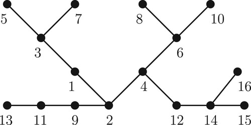
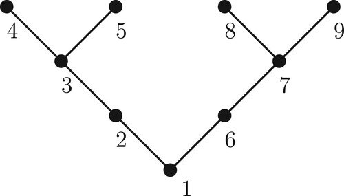
is connected. In this paper, we refer to such labelling of a tree as a successively connected labelling. The following figure depicts a successively connected labelling of a tree Figure .
Figure 1. A successively connected labelling of a tree.
In Lemma 4.3, we have seen that if the given eigenvalues are distinct, then the IEPT has a solution only if the given tree has successively connected labelling. We shall also show (Lemma 4.6) that if the given tree has successively connected labelling, then the IEPT has a solution only if the given eigenvalues are distinct. We need a few more results before that.
Lemma 4.4
Let be a monic polynomial of degree n with all real zeros and
and
be the smallest and largest zeros of P, respectively.
| (i) | If | ||||
| (ii) | If | ||||
| (iii) | If | ||||
Proof.
Follows by expressing as the product of its linear factors.
We provide a simple proof of the following strict interlacing of the extreme eigenvalues of matrices in and their principal submatrices, using Lemma 4.4.
Lemma 4.5
Let A be an real symmetric matrix such that
is a tree, and B be a
principal submatrix of A, k<n. Let α and β be the largest eigenvalues of A and B, and γ and δ be the smallest eigenvalues of A and B, respectively. Then
Proof.
We prove by induction on n that . Then, it will follow that
by comparing the largest eigenvalues of
and
, since
.
If n = 2, then is a path on two vertices. So,
with
. The only
principal submatrices of A are
and
. By Lemma 4.1,
. The characteristic polynomial of A is
. Since
, by (iii) of Lemma 4.4,
.
Assume that and that the result holds for all symmetric matrices of order less than n whose graphs are trees. Let A be an
real symmetric matrix such that
and B be the principal submatrix of A.
Putting , the characteristic polynomial of A can be written as
where the sum varies over all permutations σ of
. Since A is acyclic, the product
is non-zero only if σ is a product of disjoint two-cycles. For
let
and
denote the principal submatrices of A indexed by
and
, respectively. Then, we have
For permutations σ with , the sign of σ restricted to
is same as that of σ. Also for
,
iff
, that is the vertex
is adjacent to i. The sign of σ restricted to
, where
, is opposite to that of σ as only the two cycle
gets removed from the product of disjoint two cycles. Thus, we have
(1)
(1)
Now, let η be the largest eigenvalue of . Since each connected component of
is a subtree of
, by induction hypothesis and in view of Lemma 4.4(ii), we get
for each
. Consequently, (Equation1
(1)
(1) ) yields
. Therefore, by Lemma 4.4(iii), we get
. Thus, we have proved the result for the case when
. For any other B the argument can be repeated. This completes the proof.
We are now ready to give a necessary condition for existence of solution for the IEPT in the case of trees with successively connected labelling.
Lemma 4.6
Let T be a tree with successively connected labelling. If the IEPT has a solution, then
Proof.
Suppose be such that
and
are the smallest and the largest eigenvalues of
for
. Since
is a principal submatrix of the matrix
whose graph is a tree, so by Lemma 4.5, we have
It follows that
Lemma 4.7
Let A be a real symmetric matrix and
such that
and
are eigenvalues of
for each j. Then,
is the smallest eigenvalue and
is the largest eigenvalue of
,
.
Proof.
Follows from Cauchy's interlacing theorem.
For the rest of this section, T will denote a tree on the vertex set with successively connected labelling. We shall show that the necessary condition in Lemma 4.3 is also a sufficient condition for a solution of the IEPT for trees with successively connected labelling.
We now adopt some notations for the entries of a matrix . For a successively connected labelling, it is easy to see that for
, the vertex j is pendent in the subtree
of T induced by
. Let
. Since
is connected, degree of j is non-zero. Suppose
are adjacent to j. If
, then the unique p-q path in
along with the edges
and
produces a cycle in
, contradicting that
is a tree. Thus, j is of degree 1 in
. This allows us to define a function
given by
the unique vertex among
that is adjacent to j. Thus, for each
, the only non-zero off-diagonal entry in the jth column of
leading principal submatrix
of any matrix
is in the
th row and the only non-zero off-diagonal entry in the jth row of
is in the
th column.
The diagonal entries of A are taken to be and the off-diagonal entries
. Since A is symmetric,
for all i and j. Moreover, it follows from the above discussion that in each leading principal submatrix
,
if and only if
. Let
denote the characteristic polynomial of
,
. Further, for
, let
denote the characteristic polynomial of the principal submatrix of
obtained by deleting the rows and the columns indexed by j and
. We put
. Then, we have the following result.
Lemma 4.8
The characteristic polynomials of
satisfy the following recurrence relation:
| (i) |
| ||||
| (ii) |
| ||||
Proof.
Clearly, (i) holds. Moreover,
Now, let . In view of (Equation1
(1)
(1) ) we have
(2)
(2)
where
is the principal submatrix of A induced by
. Now, by our choice of the labelling of the vertices, the only i in
that is adjacent to j is
. Moreover,
. Hence, (Equation2
(2)
(2) ) reduces to
We therefore have the recurrence relation.
Now, for any and for
let
and
be the smallest and the largest eigenvalues of
, respectively. Then,
From Lemma 4.8 we get , and for
(3)
(3)
Thus, studying the IEPT for solutions is equivalent to seeking for appropriate solutions for the system of linear Equations (Equation3(3)
(3) ) for
and positive
. Let
be the determinant of the coefficient matrix of the system (Equation3
(3)
(3) ), i.e.
(4)
(4)
Lemma 4.9
Given a tree T with successively connected labelling and 2n−1 real numbers satisfying
there is a unique solution
of the IEPT with positive off-diagonal entries.
Proof.
We show that the systems of Equations (Equation3(3)
(3) ) can recursively be solved uniquely for real
and positive
. We put
, yielding
. Since
, for j = 2 the system becomes
which has unique solution
,
.
Now let and assume that we have obtained
and
for
so that the matrix
and the polynomials
and
are determined. Since
and
are the smallest and the largest eigenvalues of the polynomial
of degree j−1, and because
and
, in view of Lemma 4.4 we have
(5)
(5)
Let and
be the smallest and the largest zeros of the polynomial
which is of degree j−2. Then, by Lemma 4.1,
and
. Therefore, Lemma 4.4 gives
(6)
(6)
Consequently, from Equation (Equation4(4)
(4) ), we have
(7)
(7)
In particular, and therefore the system (Equation3
(3)
(3) ) has a unique solution for
and
given by
(8)
(8)
Further, from (Equation5(5)
(5) ), (Equation6
(6)
(6) ) and (Equation7
(7)
(7) ), we get
since
. Taking
as the positive square root of values obtained for
we get the unique solution we are seeking for.
Combining Lemmas 4.6 and 4.9 we get a complete answer for the IEPT for trees with successively connected labelling.
Theorem 4.10
Let T be a tree with successively connected labelling. Then, the IEPT has a solution if and only if
(9)
(9)
Further, in that case, there is a unique solution with positive off-diagonal entries. Any other solution differs from A only by signs of some off-diagonal entries.
Remark 4.1
We refer the solution A to the IEPT that has positive off-diagonal entries as the dominant solution. Since T has n−1 edges, a matrix in has n−1 pairs of equal off-diagonal entries. Thus, the IEPT has
distinct solutions in
, obtained by choosing different signs for the off-diagonal entries.
Provided the inequality (Equation9(9)
(9) ) holds, the procedures in the proof of Theorem 4.9 can be coded as a computer program which takes the eigendata and adjacency matrix (or the function
) as inputs and gives the required matrix A as output. We have coded this in SCILAB 5.5.2.
5. Numerical examples
In this section, we take up some specific examples which appeared in the papers [Citation5,Citation7–10]. We solve them using our program and find the dominant solution in each case. The values of the entries are given correct to 5 places of decimal.
Example 5.1
Consider the unlabelled tree (a broom on seven vertices) obtained by attaching three pendent vertices to one of the endpoints of a path with four vertices. Consider 13 real numbers
The tree of
labelled as in Figure was considered in [Citation5]. It is a successively connected labelling and the function v has the values
. As obtained in [Citation5], we find the dominant solution as
Figure 2. Two labellings of the broom.
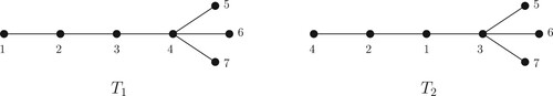
On the other hand, for the labelling of
(see Figure ), the function v takes values
. With this new v as input, the dominant solution obtained is
Note that, although the adjacency matrices of and
are permutation similar, the solutions A and
to the two IEPT with same set of eigendata are not permutation similar.
Example 5.2
Consider the tree with 12 vertices in Figure , known as a centipede. The IEPT with the 23 real numbers
was considered in [Citation7]. The function v takes values
. With these values as inputs, we get the resulting dominant solution as
which is the same as obtained in [Citation7].
Figure 3. A Labelling of the centipede C(3,5,4).
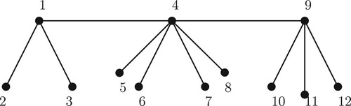
Example 5.3
Consider the generalized star T with 9 vertices shown in Figure . The tree with the eigendata
was considered in [Citation8]. The labelling is successively connected and the function v takes values
. By our program we obtain the solution as
which is the same as in [Citation8].
Figure 4. A labelling of GS(3,2,3).
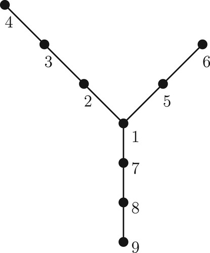
Example 5.4
Consider the tree T (called the banana tree ) with 9 vertices shown in Figure . The tree with the eigendata
was considered in [Citation9]. The labelling is successively connected and the function v takes the values
. Plugging v and the eigendata into our program we get the dominant solution as
which is same as that obtained in [Citation9].
Figure 5. A labelling of B(2,4).
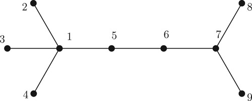
Example 5.5
Consider the tree with 9 vertices shown in Figure . The tree with the eigendata
was considered in [Citation10]. The function v takes values
,
. Plugging v and the eigendata into our program, we get the dominant solution as
which is same as that obtained in [Citation10].
Figure 6. Labelling of the vertices of .
6. Number of dominant solutions for an unlabelled tree
Let be an unlabelled tree with n vertices. For each successively connected labelling of
, we have a dominant solution of the corresponding IEPT. In this section, we discuss the number of dominant solutions that can be obtained from different successively connected labellings of
.
For let us denote by
the number of successively connected relabellings of T. We note that the dominant solution A obtained in Section 4 for a successively connected relabelling
of T is completely determined by the adjacency matrix of
. For any two successively connected relabellings of T, the dominant solutions coincide if and only if the corresponding adjacency matrices are identical. Therefore, the number of successively connected relabellings of T giving rise to the same dominant solution A is
, the number of automorphisms of T. Consequently, the number of dominant solutions obtained from different labellings of
is
.
Remark 6.1
As mentioned in Example 5.1, in all cases we have examined (including all trees with at most five vertices), we found that the dominant solutions for two labellings of an unlabelled tree whose adjacency matrices are different are not permutation similar. However, we are not sure whether this is the case in general.
Now, we need to determine the number of ways of relabelling the vertices of T such that for each
, the subgraph induced by
is a tree. Suppose
is the resulting tree through such a relabelling. Note that n is pendent in the tree
, n−1 is pendent in the tree
, and in general, j is pendent in the tree
. This observation facilitates a way for counting the number of successively connected relabellings by reducing the problem to counting the same for trees with lesser number of vertices.
Let be the set of pendent vertices of T. For
the number of successively connected relabellings of T with v as the nth vertex is
. We obtain the following recurrence relation for
.
(10)
(10)
Using the recurrence relation (Equation10(10)
(10) ), we compute the number of distinct successively connected labellings of some special trees.
6.1. The path 
Consider the path on n vertices Figure . Clearly,
. For
,
has two pendent vertices, and deletion of each of them from
results
. Thus, by repeated application of (Equation10
(10)
(10) ) gives
Figure 7. The path .
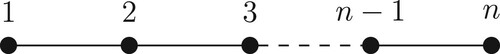
Since , the number of dominant solutions obtained from the successively connected relabellings of
is
.
6.2. The star
Let denote the star on n vertices Figure ,
. We have
. There are n−1 pendent vertices in
and deletion of each gives a star with n−1 vertices. So, by repeated application of (Equation10
(10)
(10) ), we get
Figure 8. The star .
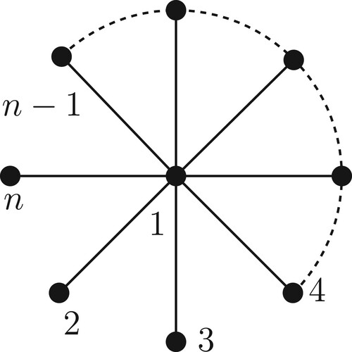
Now, the permutations of the pendent vertices produce all automorphisms of . So,
. Consequently, the number of dominant solutions obtained from the successively connected relabellings of
is 2.
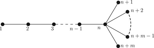
6.3. The broom (or comet)
The broom (see Figure ) has n + m vertices of which m + 1 vertices, namely,
, are pendent vertices. Since
is the path
and
is the star
, we have
and
.
Figure 9. The broom .
For , the deletion of the pendent vertex 1 from
produces
, and the deletion of each of the pendent vertices
produces
. Applying (Equation10
(10)
(10) ), we get the recurrence relation
(11)
(11)
Using (Equation11(11)
(11) ), for
we get
Similarly,
Using induction on m we show that for
(12)
(12)
Assuming our claim true for and using the recurrence relation (Equation11
(11)
(11) ) we get
Thus, for we have
Now, the permutations of the pendent vertices produce all automorphisms of
. So,
. Consequently, the number of dominant solutions obtained from the successively connected relabellings of
is given by
7. Conclusion
We have solved the IEPT completely for all trees with successively connected labellings and for the case where the given eigenvalues are distinct. The solution is primarily based on Cauchy's interlacing theorem and the recurrence relations obtained in Lemma 4.8. Trees are useful structures in graph theory as well as in computer science and methods of constructing matrices of trees having a desired eigen structure can be quite useful. The problem studied in this paper gives one such method which may also find its applications. The case for other type of labellings and for non-distinct eigenvalues can be studied further. The combinatorial problem of determining the number of distinct successively connected labellings of an arbitrary tree can also be studied further.
Acknowledgments
The authors thank the anonymous referees for their valuable comment that has enhanced the presentation of the article.
Disclosure statement
No potential conflict of interest was reported by the author(s).
Additional information
Funding
References
- Nair R, Shader BL. Acyclic matrices with a small number of distinct eigenvalues. Linear Algebra Appl. 2013;438(10):4075–4089. DOI: 10.1016/j.laa.2012.08.029.
- Peng J, Hu X, Zhang L. Two inverse eigenvalue problems for a special kind of matrices. Linear Algebra Appl. 2006;416(2):336–347. DOI: 10.1016/j.laa.2005.11.017.
- Soto RL, Pickmann H, Egana JC. Two inverse eigenproblems for symmetric doubly arrow matrices. Electron J Linear Algebra. 2009;18:700–718. DOI: 10.13001/1081-3810.1339.
- Pickmann H, Egana J, Soto RL. Extremal inverse eigenvalue problem for bordered diagonal matrices. Linear Algebra Appl. 2007;427(2):256–271. DOI: 10.1016/j.laa.2007.07.020.
- Sharma D, Sen M. Inverse eigenvalue problems for two special acyclic matrices. Mathematics. 2016;4(1):12. DOI: 10.3390/math4010012.
- Xu W-R, Chen G-L. On inverse eigenvalue problems for two kinds of special banded matrices. Filomat. 2017;31(2):371–385. ISSN 03545180, 24060933.
- Sharma D, Sen M. Inverse eigenvalue problems for acyclic matrices whose graph is a dense centipede. Special Matrices. 2018;6(1):77–92. DOI: 10.1515/spma-2018-0008.
- Heydari M, Fazeli SAS, Karbassi SM. On the inverse eigenvalue problem for a special kind of acyclic matrices. Appl Math. 2019;64(3):351–366. DOI: 10.21136/AM.2019.0242-18.
- Zarch MB, Fazeli SAS, Karbassi SM. Inverse eigenvalue problem for matrices whose graph is a banana tree. J Algor Comput. 2018;50(2):89–101.
- Babaei Zarch M, Shahzadeh Fazeli SA. Inverse eigenvalue problem for a kind of acyclic matrices. Iranian J Sci Technol, Trans A: Sci. 2019 Jul 03;2019:1–9. DOI: 10.1007/s40995-019-00737-x. First Online.
- Sharma D, Sen M. The minimax inverse eigenvalue problem for matrices whose graph is a generalized star of depth 2. Linear Algebra Appl. 2021;621:334–344. ISSN 0024-3795. DOI: 10.1016/j.laa.2021.03.021 .
- Wei Y, Dai H. An inverse eigenvalue problem for the finite element model of a vibrating rod. J Comput Appl Math. 2016;300:172–182. DOI: 10.1016/j.cam.2015.12.038.
- Nylen P, Uhlig F. Inverse eigenvalue problems associated with spring-mass systems. Linear Algebra Appl. 1997;254(1):409–425. DOI: 10.1016/S0024-3795(96)00316-3.
- Gladwel GML. Inverse problems in vibration. Dordrecht: Kluwer Academic Publishers; 2004.
- Li N. A matrix inverse eigenvalue problem and its application. Linear Algebra Appl. 1997;266:143–152. DOI: 10.1016/S0024-3795(96)00639-8.
- Fiedler M. Some inverse problems for acyclic matrices. Linear Algebra Appl. 1997;253(1):113–123.
- Horn RA, Johnson CR. Matrix analysis. New York, NY, USA: Cambridge University Press; 1986. ISBN 0-521-30586-1.
- Hogben L. Spectral graph theory and the inverse eigenvalue problem for a graph. Electron J Linear Algebra. 2005;14:12–31. DOI: 10.13001/1081-3810.1174.