Inverse boundary problem in estimating heat transfer coefficient of a round pulsating bubbly jet: design of experiment

ABSTRACT

An inverse algorithm is developed to estimate the transient convective coefficient distribution of a pulsating bubbly jet impinging on a cylindrical thermal mass. Cooling of the thermal mass is simulated by solving the two-dimensional transient heat equation in a cylindrical coordinate system using the finite difference method. The sum of squared differences between calculated and measured temperature data is the objective functional. As this is a nonlinear IHCP, the adjoint method is employed to derive the gradient components of the objective function, needed for the implementation of CGM. The procedure is carried out for six gas Reynolds numbers changing continuously through ten seconds of the jet impingement. The inverse scheme is validated using noiseless temperature data. The accuracy and convergence rate of the algorithm is then assessed by simulating the cooling process of thermal mass with four different materials. Moreover, the effects of sensors’ location, as well as initial guess on the estimation, are evaluated. Time-varying heat transfer coefficients are then estimated in the presence of Gaussian noise, having four standard deviations. Results demonstrate that, despite the estimation is affected by the noise level, the adjoint method is most efficient and rapidly convergent for the thermal mass with moderate thermal conductivity having a noisy temperature field of $\sigma$ $<$1 ${}^{\circ }\mathrm{C}$.

KEYWORDS:

• Boundary value problem
• pulsating bubbly impinging jet
• time-varying local convective heat transfer coefficient estimation
• nonlinear inverse heat conduction problem
• adjoint method
• conjugate gradient method

Nomenclature

conjugate gradient method	=	CGM
heat capacity $[\text{J}/(\text{kg K})]$	=	$C_P$
nozzle tube diameter $\text{[m]}$	=	$d$
thermal mass diameter $\text{[m]}$	=	$D$
heat transfer coefficient $[\text{W}/({\text{m}}^2\text{K})]$	=	$h$
thermal mass thickness $\text{[m]}$	=	$H$
inverse heat conduction problem	=	IHCP
thermal conductivity $[\text{W}/(\text{mK})]$	=	$k$
Lagrange function	=	$\mathcal{L}$
nozzle-to-target spacing $\text{[m]}$	=	$L$
direction of descent	=	$P$
partial differential equation	=	PDE
radial distance from stagnation point $\text{[m]}$	=	$r$
the radius of thermal mass $\text{[m]}$	=	$R$
Reynolds number $(\rho vd/\mu )$	=	$Re$
relative error (%)	=	$RE$
functional $\text{[}{\text{K}}^2]$	=	$S$
sensor	=	S
time $\text{[s]}$	=	$t$
temperature $\text{[K]}$	=	$T$
initial temperature $\text{[K]}$	=	$T_i$
variation of temperature $\text{[K]}$	=	$\mathrm{\Delta }T$
measured temperature data vector $\text{[K]}$	=	$Y$
the vertical distance from stagnation point $\text{[m]}$	=	$z$
sensitivity coefficient $\text{[}{\text{m}}^2{\text{K}}^2/\text{W]}$	=	$Z$

Subscripts

final	=	$f$
gas	=	$\text{G}$
jet	=	$j$
sensor	=	$s$

Superscripts

number of iterations	=	$i$
optimal	=	$\ast$

Greek Symbols

thermal diffusivity $\text{[}{\text{m}}^2/\text{s]}$	=	$\alpha$
step size	=	$\beta$
conjugate coefficient	=	$\gamma$
Dirac function	=	$\delta$
stopping criterion	=	${ϵ}^2$
adjoint function	=	$\lambda$
density $[\text{kg}/{\text{m}}^3]$	=	$\rho$
standard deviation	=	$\sigma$

1. Introduction

Transferring heat is a crucial requirement in many branches of metallurgical and manufacturing industries, and impinging jets are among the most effective means for cooling applications. General uses of impinging jets have been discussed in many works in the past literature [1]. Methods of improving heat transfer through impinging jets have been studied by some researchers [2–4].

Substituting a two-phase bubbly jet for a single-phase liquid jet has been demonstrated to provide a much larger heat transfer and; therefore, it seems to be an efficient method of improving heat transfer. In fact, injection of air into a liquid jet increases turbulent mixing, accelerates air–water mixture, and consequently, leads to heat transfer enhancement. Bubbly jets have been investigated experimentally by some researchers [5–9].

There are several techniques for measuring heat transfer parameters that have been addressed several times in the literature [10–12]. These techniques are effective; however, some may be difficult to implement because of limitations in initial or boundary conditions. Instead, employing methods based on solution of the inverse heat conduction problem (IHCP) is an appropriate alternative, which does not have shortcomings of conventional techniques. In this method, temperature measurement is performed with the sufficient number of thermocouples which are placed in the proper locations inside the body without making any interference with boundary layer and surface conditions. The temperature history of the body together with numerical inverse algorithms may lead us to estimate the unknown heat transfer parameters if the temperature is obtained at the appropriate location, where there is maximum sensitivity to the unknown parameters. The stability of inverse solution is extremely affected by experimental errors due to temperature measurements; therefore, IHCP is classified mathematically as being ‘ill-posed’ [13]. Several regularization and stabilization techniques have been developed to change the inverse problems to have ‘well-posed’ character [14–23].

Among many numerical inverse methods, the conjugate gradient method (CGM) together with adjoint equations lead to an efficient inverse algorithm for solving nonlinear IHCP. It is a powerful technique for function estimation and minimizing the objective functional. The adjoint method is a whole-domain, efficient algorithm with high accuracy which works by solving three sub-problems; the direct, the sensitivity, and the adjoint problems. This method has been studied by many researchers in heat transfer problems. Some notable surveys in this field can be found in Refs. [24–32].

Some investigators have already used IHCP for estimating heat transfer characteristics of a surface subjected to an impinging jet. Anderson and Singh [33] used regularization parameters together with simulated data to determine the effective heat transfer coefficients for thawing from a single impingement jet. Sagheby and Kowsary [34] designed an experiment to estimate the local convective heat transfer coefficient through a sequential procedure together with the Beck function specification approach for a slot jet impingement. Mobtil et al. [35] used Tikhonov regularization method, along with the L-curve method to determine the heat flux distribution between an impinging jet and a continuously moving flat surface. Forouzanmehr et al. [36] applied conjugate gradient method, along with backtracking line search to obtain an optimized array of four laminar impinging slot jets in order to achieve uniform distribution of heat flux over an isothermal surface. Farahani et al. [37] performed an optimization through Pattern search to achieve uniform distribution of convective heat transfer coefficient over a plate using two impinging air jets. Kowsary et al. [38] estimated the heat transfer coefficient distribution of a steady, two-phase air–water bubbly jet impinging on a cylindrical thermal mass using sequential CGM.

The authors in their previous work [32] derived the adjoint equations for the estimation of convective coefficients of cooling through mixed convection regime in a Cartesian coordinate system. In the present work, the time and space varying convective heat transfer coefficient of an unsteady pulsating bubbly flow round jet is estimated through a two-dimensional adjoint method in a cylindrical coordinate system, which has not been addressed in the previous works. Varying the gas flow with time in a pulsating manner is expected to enhance turbulence and thus heat transfer characteristics of the bubbly impinging jet. As this concept has not been considered previously, and no experimental data for this physical context is available in the literature, ‘simulated temperature data’ are generated using available correlations for the steady bubbly jet (Trainer et al. [8]) in an unsteady manner. This data is in turn fed to the derived and implemented adjoint-based CGM algorithm in order to assess the feasibility of IHCP estimation using this approach. To obtain the temperature history of the thermal mass, which is cooled by the jet, the two-dimensional, transient heat equation is solved using the finite difference method. The adjoint and sensitivity equations are then derived considering a spatially and temporally varying convective coefficient. Finally, the CGM is used to minimize the objective function, defined based on the sum of squared differences between calculated and ‘measured’ temperature data at thermocouples’ locations. Thus, to estimate time-varying convective heat transfer distribution of a pulsating bubbly impinging jet, three sets of differential equations have to be solved in a cylindrical coordinate system in every iteration before convergence criterion is satisfied: 1) the direct problem to calculate the temperature distribution of the thermal mass, 2) the sensitivity problem to determine the step size in the direction of descent, and 3) the adjoint problem to determine the gradient of the functional.

The objectives of this study are a) illustrating the effectiveness of the inverse method in assessing the accuracy of the scheme and investigating the influence of noise, b) specifying the material of the thermal mass in which the most accurate estimation of boundary condition is occurred for, c) examining the influence of sensors’ location on the performance of the inverse algorithm and d) evaluating the effect of initial guess on the estimation of 100 unknown convective coefficients with temporal and spatial variations using a significantly accurate algorithm with excellent convergence.

2. Problem statement

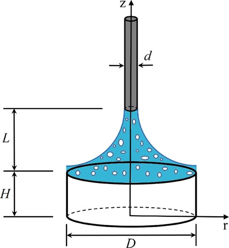
The test object is a pre-heated cylindrical-shaped thermal mass with an initial temperature of $T_i$ = 90 ${}^{\circ }\mathrm{C}$, diameter of $D$ = 10 $\text{cm}$ and a height of $H$ = 5 $\text{cm}$ as shown in Figure 1. It is insulated from peripheral and bottom sides and is instantly exposed to a bubbly impinging jet from the top surface, whose nozzle diameter is $d$ = 1 $\text{cm}$, and the nozzle-to-surface spacing is $L$ = 7 $\text{cm}$. The impinging jet is a two-phase air-assisted water jet with different values of airflow rate mixing with water. The heat conduction of the thermal mass is two-dimensional and independent of $\theta$ in a cylindrical coordinate system.

Figure 1. A cylindrical thermal mass exposed to bubbly jet impingement

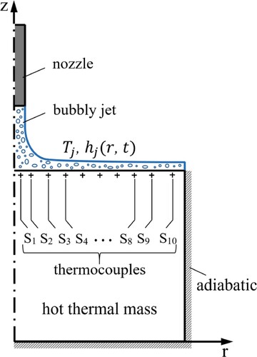
Ten thermocouples are placed 1 mm below the impingement surface along the radius of the thermal mass to record temperature data during the cooling period. Data acquisition time is considered to be 10 $\text{sec}$ with a rate of 10 $\text{Hz}$ per thermocouple. Boundary conditions and the location of thermocouples are depicted on the radial cross-section of the thermal mass in Figure 2.

Figure 2. The location of thermocouples inside an insulated thermal mass exposed to $h_j(r,t)$

In order to simulate the impinging jet experiment and to obtain temperature history recorded by thermocouples, the convective coefficients of the two-phase bubbly jet $(h_j)$ are extracted from the experimental data of Ref. [8]. However, the data of Ref. [8] is given at steady state condition while in this study, we assume that the airflow rate changes in every second of jet impingement. In other words, despite using convective heat transfer coefficients obtained by Trainer et al. [8] for six different gas Reynolds numbers (which represents six different gas flow rates), these data are employed in the transient condition in which the gas flow rate of the bubbly jet varies continuously during the cooling period. Hence, the convective heat transfer coefficients of the pulsating impinging jet will be modeled as a function of both space (i.e. radial location) and time $(h_j(r,t))$.

3. Simulation of the experiment

Figure 3 shows heat transfer distributions of the bubbly jet extracted from the experimental study of Ref. [8] at six gas Reynolds numbers $(R{e}_G)$. In this work, the experimental data are approximated by an eight-degree polynomial for all gas Reynolds numbers, as shown in Figure 3.

Figure 3. The heat transfer distributions in experimental studies of Ref. [8] at six gas Reynolds numbers

Figure 4 shows the manner by which the gas Reynolds number of the bubbly jet varies during 10 sec of cooling. Applying this variation in $R{e}_G$ results the convective components of the bubbly jet to be fluctuating as shown in Figure 5. Consequently, the simulation of the experiment is performed in the transient condition with a spatially and temporally varying convective heat transfer coefficient for the pulsating bubbly jet $(h_j(r,t))$.

Figure 4. Variation of gas Reynolds number with time

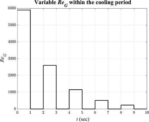
Figure 5. Time-varying convective coefficient components of the bubbly jet

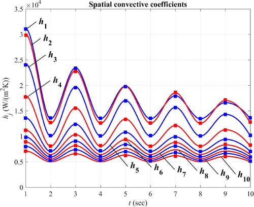
Convective heat transfer coefficient $h_j(r,t)$ is discretized into ten components $(h_1,h_2,\dots ,h_{10})$ through spatial averaging in ten intervals over the radius of the thermal mass in every second of cooling. The radial intervals are nonuniform and more packed around the jet stagnation point, where maximum heat transfer occurs. Ten thermocouples are ‘placed’ along the radius of the thermal mass, 1 mm below the impingement surface in the middle of each interval, in order to record the temperature data during the cooling period (Figure 2). Choosing equal numbers of sensors and convective coefficient components gives one the opportunity of examining the solution algorithm at the threshold of its capacity. Figure 6 shows the manner by which $h_j$-curve is discretized to obtain local components along the radius of the thermal mass at $t$ = 1 $\text{sec}$ when jet impinges with gas Reynolds number of $R{e}_G$ = 5900. The same discretization method has been employed to $h_j$-curves in other times over the radius of thermal mass. The values of $h_j$-components during the jet impingement are given in Table 1.

Figure 6. Discretization of $h_j$-curve to local components along the radius of thermal mass

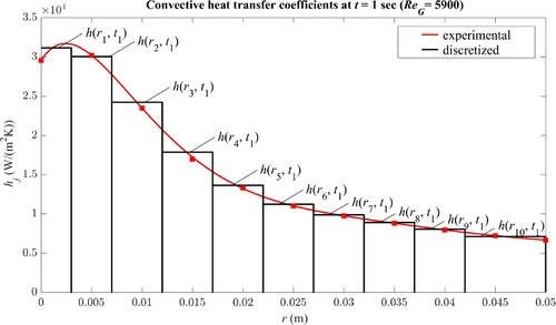
Table 1. Discretized values of $h_j$ over ten seconds of cooling

	${\mathit{h}}_{\mathit{j}}(\mathbf{W}/({\mathbf{m}}^2\mathbf{K}))$
$\mathit{t}\mathit{i}\mathit{m}\mathit{e}(\mathbf{s}\mathbf{e}\mathbf{c})$	${\mathit{h}}_1$	${\mathit{h}}_2$	${\mathit{h}}_3$	${\mathit{h}}_4$	${\mathit{h}}_5$	${\mathit{h}}_6$	${\mathit{h}}_7$	${\mathit{h}}_8$	${\mathit{h}}_9$	${\mathit{h}}_{10}$
$1$	31138.8	30030.2	24211.2	17860.0	13619.7	11227.9	9862.1	8893.0	8038.1	7111.1
$2$	13432.6	12547.4	10036.4	8047.2	7025.7	6417.8	5941.8	5556.7	5252.8	4988.8
$3$	23446.5	22940.2	19704.5	15590.4	12391.7	10344.3	9081.5	8170.9	7390.0	6580.3
$4$	13432.6	12547.4	10036.4	8047.2	7025.7	6417.8	5941.8	5556.7	5252.8	4988.8
$5$	19867.0	19786.0	17039.3	13397.8	10808.3	9351.5	8427.8	7651.8	7011.4	6343.9
$6$	13432.6	12547.4	10036.4	8047.2	7025.7	6417.8	5941.8	5556.7	5252.8	4988.8
$7$	17967.3	18538.1	15707.6	12138.6	9916.4	8819.1	8084.7	7372.7	6782.0	6205.8
$8$	13432.6	12547.4	10036.4	8047.2	7025.7	6417.8	5941.8	5556.7	5252.8	4988.8
$9$	16620.5	17052.3	14321.9	11295.6	9398.7	8323.5	7637.8	7109.9	6639.7	6071.1
$10$	13432.6	12547.4	10036.4	8047.2	7025.7	6417.8	5941.8	5556.7	5252.8	4988.8

Finally, the heat transfer of the variable flow bubbly impinging jet is obtained for ten seconds of the cooling period while the heat conduction of the thermal mass is assumed to be two-dimensional in an axisymmetric coordinate system.

Now, by specifying the boundary conditions of the thermal mass at the top, bottom and peripheral sides and knowing the thermophysical properties and initial condition, temperature distribution can be obtained through the domain by solving the direct heat conduction problem.

3.1. The direct cooling problem with jet impingement

The two-dimensional, transient heat conduction equation in an axisymmetric coordinate system together with initial and boundary conditions are given as (1) $\begin{array}{rl}\frac{1}{r}\frac{\mathrm{\partial }}{\mathrm{\partial }r}\left(r\frac{\mathrm{\partial }T}{\mathrm{\partial }r}\right)+\frac{{\mathrm{\partial }}^{2}T}{\mathrm{\partial }{z}^2}& =\frac{1}{\alpha }\frac{\mathrm{\partial }T}{\mathrm{\partial }t}\end{array}$(1) (2) $\begin{array}{rl}T=T_i,att& =0\end{array}$(2) (3) $\begin{array}{rl}\frac{\mathrm{\partial }T}{\mathrm{\partial }r}& =0,atr=0\end{array}$(3) (4) $\begin{array}{rl}\frac{\mathrm{\partial }T}{\mathrm{\partial }r}& =0,atr=R\end{array}$(4) (5) $\begin{array}{rl}\frac{\mathrm{\partial }T}{\mathrm{\partial }z}& =0,atz=0\end{array}$(5) (6) $\begin{array}{rl}-k\frac{\mathrm{\partial }T}{\mathrm{\partial }z}& =h_j(r,t)(T-T_j),atz=H.\end{array}$(6)

Assuming that the thermal properties of the material are independent of temperature, geometry and boundary conditions used are shown in Figures. 1 and 2, respectively.

In the above equations, $\alpha$ is the thermal diffusivity of carbon steel thermal mass with a radius of $R$ = 5 $\text{cm}$ and height of $H$ = 5 $\text{cm}$, which is exposed to the bubbly jet with a temperature of $T_j$ = 25 ${}^{\circ }\mathrm{C}$. The values for time–space varying convective coefficients $h_j(r,t)$, are substituted from Table 1 considering the relevant cooling time.

The governing equations subjected to initial and boundary conditions are solved by the finite difference method. The spatial domains are discretized using uniform rectangular computational cells. The second-order central differencing scheme has been used for the discretization of diffusion terms and boundary conditions. The transient heat equation is solved explicitly. The time step and cells dimensions are chosen in such a way that the stability criteria in numerical solution are satisfied. The grid independence test has been carried out for three different grid sizes, namely, 25×25, 50×50 and 100×100. Based on this comparison, a 50×50 grid has been chosen for obtaining the results.

3.2. Generation of simulated data

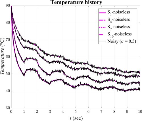
In order to estimate the unknown heat transfer coefficient of a pulsating two-phase bubbly jet by the inverse technique, it is required to generate realistic experimental data at measurement points during jet impingement. For this purpose, the normally distributed random values with a specific standard deviation are added to the simulated temperatures obtained from the solution of the direct problem, resulting in noisy simulated temperatures.

Random Gaussian errors with four standard deviations of $\sigma$ = 0.05 ${}^{\circ }\mathrm{C}$, $\sigma$ = 0. 1 ${}^{\circ }\mathrm{C}$, $\sigma$ = 0.5 ${}^{\circ }\mathrm{C}$ and $\sigma$ = 1 ${}^{\circ }\mathrm{C}$ are added to the calculated data. The result is considered as measured temperature $(Y(r,t))$ recorded by ten sensors in every 0.1 s of the cooling period. Figure 7 shows the noiseless and noisy simulated temperature history of thermal mass at four measurement points (S₁, S₄, S₇ and S₁₀) with $\sigma$ = 0.5 ${}^{\circ }\mathrm{C}$ during ten seconds of jet impingement.

Figure 7. The noiseless and noisy simulated temperature history of thermal mass at four measurement points

4. Inverse estimation

In this work, the inverse problem is of boundary estimation type, as the convective coefficient of the top boundary is the unknown and should be estimated through minimization of the objective function$S$ defined as (7) $\begin{array}{r}S[h_j(r,t)]=\underset{0}{\overset{t_f}{\int }}\underset{0}{\overset{H}{\int }}\underset{0}{\overset{R}{\int }}(T(r,z,t;h_j)-Y(r,z,t){)}^2\delta (r-r_s)\delta (z-z_s)drdzdt.\end{array}$(7) In the above equation, $T$ is the function of calculated temperatures as obtained from the solution of the direct problem, $Y$ is the function containing ‘measured’ temperature data at different times, $\delta (.)$ is the Dirac function which is used for punctual discrete measurements at sensors locations ($r_s$, $z_s$) and $t_f$ refers to the duration of the experiment.

In the adjoint method, three groups of equations must be solved in every iteration before the convergence criterion to be satisfied. These equations are: 1) the direct problem to calculate the temperature distribution over the thermal mass, 2) the sensitivity problem to determine the optimal step size in the direction of descent, and 3) the adjoint problem to determine the gradient of the functional used to evaluate the descent direction.

4.1. The adjoint problem

In this inverse problem, we want to determine convective coefficient components of $h_j(r,t)$ which minimizes the sum of squared errors through numerical solutions. Accordingly, it is essential to add the transient heat conduction equation as a physical constraint to the functional $S$ via Lagrange multiplier function $\lambda$ and form the Lagrange function as (8) $\begin{array}{rl}\mathcal{L}(T,h_j)& =\underset{0}{\overset{t_f}{\int }}\underset{0}{\overset{H}{\int }}\underset{0}{\overset{R}{\int }}(T(r,z,t)-Y(r,z,t){)}^2\delta (r-r_s)\delta (z-z_s)drdzdt\\ & +\underset{0}{\overset{t_f}{\int }}\underset{0}{\overset{H}{\int }}\underset{0}{\overset{R}{\int }}\lambda (r,z,t)\left\{\frac{1}{\alpha }\frac{\mathrm{\partial }T}{\mathrm{\partial }t}-\frac{{\mathrm{\partial }}^{2}T}{\mathrm{\partial }{r}^2}-\frac{1}{r}\frac{\mathrm{\partial }T}{\mathrm{\partial }r}-\frac{{\mathrm{\partial }}^{2}T}{\mathrm{\partial }{z}^2}\right\}rdrdzdt.\end{array}$(8) Performing integration by parts, applying initial and boundary conditions from Eqs. (2) to (6), and some rearrangements the Lagrange function becomes (9) $\begin{array}{rl}\mathcal{L}& =\underset{0}{\overset{t_f}{\int }}\underset{0}{\overset{H}{\int }}\underset{0}{\overset{R}{\int }}(T-Y{)}^2\delta (r-r_s)\delta (z-z_s)drdzdt-\underset{0}{\overset{t_f}{\int }}\underset{0}{\overset{H}{\int }}\underset{0}{\overset{R}{\int }}T\left\{\frac{r}{\alpha }{\lambda }_t+r{\lambda }_{rr}+{\lambda }_r+r{\lambda }_{zz}\right\}\\ & drdzdt+\underset{0}{\overset{H}{\int }}\underset{0}{\overset{R}{\int }}{\frac{r}{\alpha }T\lambda ]}_{t=t_f}drdz+\underset{0}{\overset{t_f}{\int }}\underset{0}{\overset{H}{\int }}T\{r{{\lambda }_r]}_{r=R}-{r{\lambda }_r]}_{r=0}\}dzdt+\\ & \underset{0}{\overset{t_f}{\int }}\underset{0}{\overset{R}{\int }}\left\{rT({{\lambda }_z]}_{z=H}-{{\lambda }_z]}_{z=0})+{\frac{r\lambda h_j}{k}(T-T_j)]}_{z=H}\right\}drdt.\end{array}$(9) Taking the differential of the Lagrange function results in variations $\delta T$ and $d{h}_j$ in the form given by (10) $\begin{array}{rl}d\mathcal{L}& =\underset{0}{\overset{t_f}{\int }}\underset{0}{\overset{H}{\int }}\underset{0}{\overset{R}{\int }}\{2(T-Y)\delta (r-r_s)\delta (z-z_s)-\}\\ & \times \left(\frac{r}{\alpha }{\lambda }_t+r{\lambda }_{rr}+{\lambda }_r+r{\lambda }_{zz}\right)\}\delta Tdrdzdt+\underset{0}{\overset{H}{\int }}\underset{0}{\overset{R}{\int }}{\frac{r}{\alpha }\lambda ]}_{t=t_f}\delta Tdrdz\\ & +\underset{0}{\overset{t_f}{\int }}\underset{0}{\overset{H}{\int }}\{r{{\lambda }_r]}_{r=R}-r{{\lambda }_r]}_{r=0}\}\delta Tdzdt\\ & +\underset{0}{\overset{t_f}{\int }}\underset{0}{\overset{R}{\int }}r\left\{({{\lambda }_z]}_{z=H}-{{\lambda }_z]}_{z=0})+{\frac{\lambda h_j}{k}]}_{z=H}\right\}\delta Tdrdt\\ & +\underset{0}{\overset{t_f}{\int }}\underset{0}{\overset{R}{\int }}{\frac{r\lambda }{k}(T-T_j)]}_{z=H}d{h}_{j}drdt.\end{array}$(10) Hence, the adjoint differential equation along with initial (i.e. final) and boundary conditions are obtained as (11) $\begin{array}{rl}r({\lambda }_{rr}+\frac{1}{r}{\lambda }_r+{\lambda }_{zz}+\frac{1}{\alpha }{\lambda }_t)& =2(T-Y)\delta (r-r_s)\delta (z-z_s)\end{array}$(11) (12) $\begin{array}{rl}\lambda =0,att& =t_f\end{array}$(12) (13) $\begin{array}{rl}\lambda =0,atr& =0\end{array}$(13) (14) $\begin{array}{rl}{\lambda }_r=0,atr& =R\end{array}$(14) (15) $\begin{array}{rl}{\lambda }_z=0,atz& =0\end{array}$(15) (16) $\begin{array}{rl}-k{\lambda }_z& =h_j(r,t)\lambda ,atz=H.\end{array}$(16)

These equations are solved backward in time by integrating from the final time $t_f$ down to the initial time using the finite difference method. The Dirac function in Eq. (11) implies that source terms are discrete and located at each sensor location ($r_s$, $z_s$).

Consequently, when the adjoint differential equation is satisfied, Eq. (10) is simplified as (17) $\begin{array}{r}d\mathcal{L}=\underset{0}{\overset{t_f}{\int }}\underset{0}{\overset{R}{\int }}\frac{r\lambda (r,H,t)}{k}(T(r,H,t)-T_j)d{h}_{j}drdt.\end{array}$(17) As $T$ is the solution of the heat equation, the components of the gradient vector of the functional can be computed from the gradient of the Lagrange function. As a result, the gradient of the functional is given by (18) $\begin{array}{r}\mathrm{\nabla }S=\frac{r\lambda (r,H,t)}{k}(T(r,H,t)-T_j).\end{array}$(18) The conjugate gradient method minimizes the functional in a whole time-domain procedure using the values of functional gradient [17].

4.2. The sensitivity problem

To derive the sensitivity equation, temperature function $T(r,z,t)$ is replaced by $T+\mathrm{\Delta }T$ in the heat equation. $\mathrm{\Delta }T$ is the variation of $T$ in the direction of descent. By subtracting the resulting PDE from the original heat equation, and after some manipulations, the sensitivity equation is obtained as (19) $\begin{array}{rl}\frac{{\mathrm{\partial }}^2\mathrm{\Delta }T}{\mathrm{\partial }{r}^2}+\frac{1}{r}\frac{\mathrm{\partial }\mathrm{\Delta }T}{\mathrm{\partial }r}+\frac{{\mathrm{\partial }}^2\mathrm{\Delta }T}{\mathrm{\partial }{z}^2}& =\frac{1}{\alpha }\frac{\mathrm{\partial }\mathrm{\Delta }T}{\mathrm{\partial }t}\end{array}$(19) (20) $\begin{array}{rl}\mathrm{\Delta }T=0,att& =0\end{array}$(20) (21) $\begin{array}{rl}\frac{\mathrm{\partial }\mathrm{\Delta }T}{\mathrm{\partial }r}& =0,atr=0\end{array}$(21) (22) $\begin{array}{rl}\frac{\mathrm{\partial }\mathrm{\Delta }T}{\mathrm{\partial }r}& =0,atr=R\end{array}$(22) (23) $\begin{array}{rl}\frac{\mathrm{\partial }\mathrm{\Delta }T}{\mathrm{\partial }z}& =0,atz=0\end{array}$(23) (24) $\begin{array}{rl}-k\frac{\mathrm{\partial }\mathrm{\Delta }T}{\mathrm{\partial }z}& =\mathrm{\Delta }{h}_j(r,t)(T+\mathrm{\Delta }T-T_j)+h_j(r,t)\mathrm{\Delta }T,atz=H.\end{array}$(24)

4.3. The conjugate gradient method

The conjugate gradient method (CGM) is an optimization technique used to estimate the components of the convective coefficient by minimizing the objective function defined by Eq. (7). The iterative procedure using the CGM is summarized by (25) $\begin{array}{r}{h}_j^{i+1}=h_j^i+{{\beta }^{\ast }}^i{P}^i,\end{array}$(25) where the direction of descent, $P^i$, in the design space at the $i$^th iteration is defined as (26) $\begin{array}{r}{P}^i=-\mathrm{\nabla }{S}^i+{\gamma }^i{P}^{i-1},\end{array}$(26) and the conjugate coefficient, ${\gamma }^i$, is calculated as (27) $\begin{array}{r}\{\begin{array}{c}{\gamma }^i=0;i=1\\ {\gamma }^i={\displaystyle \frac{{\int }_0^{t_f}{\int }_0^R{[\mathrm{\nabla }{S}^i]}^{2}drdt}{{\int }_0^{t_f}{\int }_0^R{[\mathrm{\nabla }{S}^{i-1}]}^{2}drdt}};i>1.\end{array}\end{array}$(27) The optimal step size, ${\beta }^{\ast }$, in the direction of descent, $P^i$, is obtained by minimizing the functional in the search direction with respect to the step size. Thus, by setting (28) $\begin{array}{r}\frac{\mathrm{\partial }{S}^{i+1}}{\mathrm{\partial }{\beta }^i}=0,\end{array}$(28) And, after some algebraic manipulations, the optimal step size is calculated using (29) $\begin{array}{r}{{\beta }^{\ast }}^i=\frac{{\int }_0^{t_f}{\int }_0^H{\int }_0^R\mathrm{\Delta }T(T-Y)\delta (r-r_s)\delta (z-z_s)drdzdt}{{\int }_0^{t_f}{\int }_0^H{\int }_0^R{(\mathrm{\Delta }T)}^2\delta (r-r_s)\delta (z-z_s)drdzdt}.\end{array}$(29)

4.4. Stopping Criterion

As the CGM is iterative, a suitable criterion is required to terminate the iterations. Here, the discrepancy of the experimental temperature data (30) $\begin{array}{r}{ϵ}^2=\underset{0}{\overset{t_f}{\int }}{\sigma }^{2}dt,\end{array}$(30) is considered as the convergence criterion through the standard deviation of the measured data [28]. The iteration process is terminated when (31) $\begin{array}{r}S[h_j(r,t)]<{ϵ}^2.\end{array}$(31) For non-noisy temperature data, the convergence criterion could be chosen as a minimum value. In the present work, ${ϵ}^2$ = 0.0001 is used.

4.5. The solution algorithm

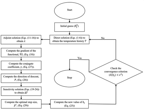
The statement of the full inverse algorithm can be summarized as follows [32]:

1. Provide an initial guess to the convective heat transfer coefficients $(h_j^0)$.

2. Solve the direct heat conduction problem (Eqs. (1-6)) to obtain the temperature distribution through the thermal mass.

3. Solve the adjoint problem (Eqs. (11-16)) to obtain $\lambda (r,z,t)$.

4. Compute the gradient of the functional, $\mathrm{\nabla }S$, (Eq. (18)).

5. Compute the conjugate coefficient, $\gamma$, (Eq. (27)).

6. Compute the direction of descent, $P$, (Eq. (26)).

7. Solve the sensitivity problem (Eqs. (19-24)).

8. Compute the optimal step size, ${\beta }^{\ast }$, (Eq. (29)).

9. Compute the new value of $h_j$ (Eq. (25)).

10. Check the convergence criterion. If it is not satisfied, go to step 2 with updated $h_j$.

The flow diagram for steps 1 through 10 (above) is presented in Figure 8.

Figure 8. The flow diagram of the adjoint-based CGM algorithm

5. Results and discussion

In order to validate the inverse method, the components of the convective coefficient of the pulsating bubbly impinging jet are estimated using noiseless temperature data. The relative error, $RE$, is defined as (32) $\begin{array}{r}RE(\mathrm{\%})=\left|\frac{h_{j,estimated}-h_{j,exact}}{h_{j,exact}}\right|\times 100,\end{array}$(32) for all estimated convective components are given in Table 2.

Table 2. Relative error of all $h_j$-components using noiseless temperature data

	$\mathit{R}\mathit{E}(\mathrm{\%})$
$\mathit{t}\mathit{i}\mathit{m}\mathit{e}$ $(\mathbf{s}\mathbf{e}\mathbf{c}$)	${\mathit{h}}_1$	${\mathit{h}}_2$	${\mathit{h}}_3$	${\mathit{h}}_4$	${\mathit{h}}_5$	${\mathit{h}}_6$	${\mathit{h}}_7$	${\mathit{h}}_8$	${\mathit{h}}_9$	${\mathit{h}}_{10}$
$1$	0.00038	0.00019	0.00008	0.00002	0.00004	0.00003	0.00007	0.00005	0.00001	0.00002
$2$	0.00028	0.00025	0.00004	0.00015	0.00010	0.00001	0.00001	0.00000	0.00004	0.00010
$3$	0.00007	0.00051	0.00006	0.00001	0.00003	0.00003	0.00004	0.00011	0.00005	0.00000
$4$	0.00061	0.00016	0.00011	0.00014	0.00011	0.00002	0.00005	0.00009	0.00007	0.00005
$5$	0.00110	0.00059	0.00020	0.00014	0.00000	0.00001	0.00011	0.00001	0.00018	0.00001
$6$	0.00074	0.00021	0.00011	0.00009	0.00013	0.00007	0.00005	0.00011	0.00007	0.00003
$7$	0.00077	0.00056	0.00020	0.00012	0.00012	0.00005	0.00013	0.00005	0.00016	0.00002
$8$	0.00075	0.00040	0.00025	0.00015	0.00013	0.00004	0.00046	0.00007	0.00006	0.00005
$9$	0.00008	0.00006	0.00003	0.00009	0.00001	0.00014	0.00025	0.00001	0.00005	0.00003
$10$	0.00034	0.00009	0.00004	0.00001	0.00006	0.00005	0.00007	0.00007	0.00000	0.00012

As mentioned previously, the exact $h_j$’ s $(h_{j,exact})$ in Eq. (32), are the convective coefficients extracted from the experimental data of Ref. [8].

It is clear from the Table that errors are very low and less than 0.0012% for all convective components showing the excellent agreement between the inverse estimation and exact $h_j$.

5.1. The effect of thermal mass material

To estimate the convective coefficients of the bubbly jet through an inverse algorithm, the first step is to calculate temperature distribution inside the pre-heated thermal mass while it is exposed to jet impingement. Hence, it is expected that the estimation is affected by the thermal mass material. To assess the performance of the inverse algorithm, four different materials are chosen as the thermal mass: 1- copper, 2- carbon steel, 3- chromium steel and 4- stainless steel. The thermophysical properties of these materials at the initial temperature of $T_i$ = 90 ${}^{\circ }\mathrm{C}$ are provided in Table 3.

Table 3. Thermophysical properties of four different thermal mass materials

Properties	Copper	Carbon steel	Chromium steel	Stainless steel
$k(\mathrm{W}/(\mathrm{mK}))$	401	60.5	37.7	14.9
$\rho (\mathrm{kg}/{\mathrm{m}}^3)$	8933	7854	7822	7900
$C_p(\mathrm{J}/(\mathrm{kgK}))$	385	434	444	477

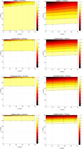
Figure 9 shows the temperature contours inside these four thermal mass materials in a radial cross-section of the body at two cooling times when the initial temperature is $T_i$ = 90 ${}^{\circ }\mathrm{C}$. It is clear from the figure that, despite all four thermal masses are subjected to the bubbly jet with equal spatial and temporal convective coefficients, the cooling rate is different for each one due to the different thermophysical properties of the materials.

Figure 9. The temperature contours of cylindrical thermal mass, all in degrees Celsius

The convergence history of the objective functional $S$ is depicted in Figure 10 for the mentioned materials when the estimation is carried out with the noiseless temperature data. The initial guess is $(h_j^0{)}_{i,k}$ = 10000 ($i$ = $k$ = 1, … , 10) for all 100 components of the convective coefficient matrix. It is obvious from the figure that, for all materials, the convergence curves descend fast in the initial iterations; however, the best inverse optimization is attributed to the carbon steel thermal mass with the largest reduction of $S$ to 2e-6. Both increase and decrease of the thermal conductivity in the other materials as compared to carbon steel causes less reduction of $S$, which means a higher estimation error via the inverse scheme.

Figure 10. The trend of convergence of the inverse algorithm for four thermal mass materials

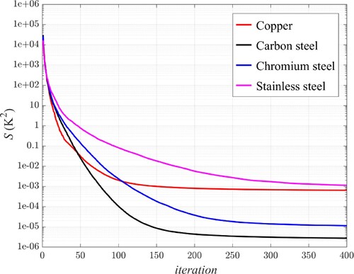
Consequently, moderate heat-conducting metals, such as carbon steel, are more appropriate to be used in the inverse technique, since high heat-conducting metals, such as copper, will result in a very small temperature gradient within the body, which will cause the inverse heat conduction algorithm not to execute properly. It is due to the fact that, the top surface of copper thermal mass cools down exposed to jet impingement, drawing heat from other parts of the body. Therefore, temperature drops throughout the thermal mass resulting the top surface not only to be affected by cooling from above (jet impingement) but also by heating from the bottom of thermal mass due to the low temperature gradient. On the other hand, low heat-conducting metals, such as stainless steel, with high temperature gradient will cause the temperature of the thermal mass drops rapidly on the impingement surface only, while the rest of thermal mass remains hot during cooling period (Figure 9). Therefore, the temperature difference between the jet and the impingement surface decreases, causes less variation of temperature at measurement points due to jet impingement. These explanations imply the effect of ‘sensitivity coefficient’ in inverse analysis.

The sensitivity coefficient $(Z)$ which is defined as ‘the derivative of temperature at the m^th sensor with respect to the n^th component of the convective coefficient’, simply specifies the best material for inverse estimation. The absolute value of the sensitivity coefficient is depicted in Figure 11 for the first array of the sensitivity coefficients matrix $(Z_{11}=\frac{\mathrm{\partial }{T}_1}{\mathrm{\partial }{h}_1})$ and the last one $(Z_{1010}=\frac{\mathrm{\partial }{T}_{10}}{\mathrm{\partial }{h}_{10}})$, since other arrays of $Z_{ii}$ ($i$ = 2, … , 8) fall between these two values with similar sequential order in four thermal mass materials.

Figure 11. The absolute value of the two sensitivity coefficients in four thermal mass materials

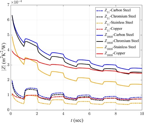
As it is shown in Figure 11, the sensitivity coefficients for carbon steel are of the largest values compared to the other materials with both higher and lower thermal conductivity during ten seconds of jet impingement. It is also worth noting from Figures 10 and 11 that, the larger the sensitivity coefficient, the lower the estimation error.

5.2. The effect of sensors’ location

Since IHCP is classified as an ill-posed problem, it is highly sensitive to the location of measurement points. Therefore, another important factor that should be considered in the design of the experiment, is to choose the best place for locating sensors in a manner to impose the least error of estimation to the calculations. For this purpose, we assume I) different distances between measurement points radially and II) different distances between measurement points and the impingement surface, and evaluate the influence of sensors’ location on the results.

The determination of the best location for the sensors on the radius of the thermal mass is an optimization problem by itself. However, to address this issue, the numerical code is implemented for three different cases with the initial guess of $(h_j^0{)}_{10\times 10}=5000$ for all 100 components of convective coefficients while measurement points are 1 mm below the active surface: I-a) ten sensors to be located in the middle of each discretized interval (explained in section 3, also see Figure 6), I-b) ten sensors to be located at the endpoint of each interval and I-c) ten sensors to be located at the beginning point of each interval. The convergence history of the objective functional S is depicted in Figure 12 for carbon steel thermal mass when the estimation is carried out with the noiseless temperature data.

Figure 12. The trend of convergence of the inverse algorithm for three different sensor arrangements

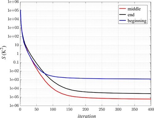
It is clear from Figure 12 that the best inverse estimation is attributed to case (I-a) in which the sensors are located in the middle of each interval. Every other arrangement will impose additional bias error to the optimization; however, by locating sensors at the endpoint of each interval, the error is not that bad when compared with the error of placing the sensors in the middle of the interval.

To examine the effect of distance between measurement points and the impingement surface, calculations are performed with the same initial guess mentioned above while considering three different cases: II-a) ten sensors to be located 1 mm below the active surface, II-b) ten sensors to be located 2 mm below the active surface and II-c) ten sensors to be located 3 mm below the active surface when all sensors are located in the middle of each interval. The convergence history of the objective functional S is illustrated in Figure 13 for carbon steel thermal mass when the estimation is carried out with the noiseless temperature data.

Figure 13. The trend of convergence of the inverse algorithm for three different sensor distances from the active surface

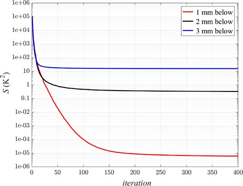
As it is shown in Figure 13, the least error occurs for case (II-a) in which sensors are located 1 mm below the active surface. As the measurement distance from the active surface increases, a considerable estimation error will be imposed on the optimization.

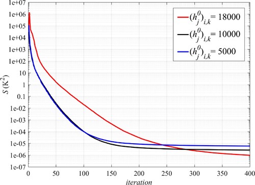
5.3. The effect of initial guess

To examine the behavior of the inverse scheme, different values of convective coefficients are fed to the algorithm as the initial guess. The developed inverse code is executed with noiseless temperature data ($\sigma$ = 0) for carbon steel thermal mass with three initial guesses $(h_j^0{)}_{i,k}$ = 5000, $(h_j^0{)}_{i,k}$ = 10000 and $(h_j^0{)}_{i,k}$ = 18000 ($i$ = $k$ = 1, … , 10) for all 100 components of the convective coefficient matrix. The convergence history of the objective functional $S$ is presented in Figure 14. It is obvious from the figure that, the initial guess affects the convergence rate and the converged value of $S$; however, it is not that remarkable since the converged values of $S$ in all three cases are below the termination value ($S$ < 0.0001). As a result, the estimation will not be greatly compromised by changes in the initial guess.

Figure 14. The trend of convergence for three initial guesses

5.4. The effect of measurement noise level

Here, the influence of the temperature noise level on the accuracy of the estimation is examined for carbon steel thermal mass considering noisy temperature data with four standard deviations of $\sigma$ = 0.05 ${}^{\circ }\mathrm{C}$, $\sigma$ = 0. 1 ${}^{\circ }\mathrm{C}$, $\sigma$ = 0.5 ${}^{\circ }\mathrm{C}$ and $\sigma$ = 1 ${}^{\circ }\mathrm{C}$.

Figures 15–18 show temporal and spatial variation of four $h_j$-components for the exact (solid lines) and estimated (dashed-dotted lines) convective coefficients using noisy temperature data with standard deviations of $\sigma$ = 0.05 ${}^{\circ }\mathrm{C}$, $\sigma$ = 0. 1 ${}^{\circ }\mathrm{C}$, $\sigma$ = 0.5 ${}^{\circ }\mathrm{C}$ and $\sigma$ = 1 ${}^{\circ }\mathrm{C}$, respectively. These $h_j$-components are chosen in a manner to have the most transparency from a graphical presentation point of view. It is observed from these figures that noisy temperature data causes some discrepancies in the estimation. The error is negligible at $\sigma$ = 0.05 ${}^{\circ }\mathrm{C}$; however, by increasing $\sigma$ to higher values, the fluctuations around the exact data amplifies; resulting in the average relative errors of 0.00014%, 4.76% and 9.70% for $\sigma$ = 0. 1, $\sigma$ = 0.5 and $\sigma$ = 1 ${}^{\circ }\mathrm{C}$, respectively.

Figure 15. Exact and estimated convective coefficients using noisy data with $\sigma$ = 0.05 ${}^{\circ }\mathrm{C}$

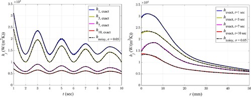
Figure 16. Exact and estimated convective coefficients using noisy data with $\sigma$ = 0.1 ${}^{\circ }\mathrm{C}$

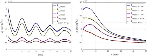
Figure 17. Exact and estimated convective coefficients using noisy data with $\sigma$ = 0.5 ${}^{\circ }\mathrm{C}$

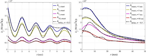
Figure 18. Exact and estimated convective coefficients using noisy data with $\sigma$ = 1 ${}^{\circ }\mathrm{C}$

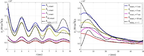
It is also worth noting that noise does not affect all convective coefficients similarly; Comparing estimated coefficients at bigger $\sigma$ reveals that the larger deviation from the exact value is attributed to the bigger components of convective coefficient $(h_1,h_3)$ at the stagnation region where the heat transfer is of maximum value. It is because, higher values of convective coefficients have lower sensitivities to temperature variation during the cooling period and, consequently, larger estimation errors are attributed to them in the inverse scheme.

Furthermore, at higher data acquisition times which the temperature difference between the bubbly jet and thermal mass decreases, the error of estimation increases due to the decline of sensitivity. Comparing the results obtained from noisy temperature data with four $\sigma$’ s indicates that, at least in this case study, results are not affected appreciably with an increasing standard deviation of the noise. It should however be noted that increasing $\sigma$ to a value as high as 1 ${}^{\circ }\mathrm{C}$ causes big estimation errors in predicting the components of the convective coefficient of the variable flow bubbly jet using the present inverse algorithm.

6. Conclusions

A two-dimensional nonlinear IHCP is implemented to directly predict the local convective heat transfer coefficient of the pulsating bubbly flow round jet impinges on a heated cylindrical thermal mass. The airflow rate of the bubbly jet altered in every second of jet impingement during 10 s of cooling which made the heat transfer occur unsteadily through time–space varying convective heat transfer coefficient at the top boundary of thermal mass. The cooling process was simulated by solving transient heat conduction equations in the cylindrical coordinate system using the finite difference method. The adjoint method was employed to estimate the convective coefficients by minimizing the sum of squared errors as the functional using the conjugate gradient method.

The inverse method was validated using exact temperature data without noise. Results showed an excellent agreement between estimated and exact convective coefficients with less than 0.0012% relative error for all convective components showing the excellent performance of the inverse scheme in estimating ten local convective coefficients $(h_1,h_2,\dots ,h_{10})$ in every second of the cooling period over ten seconds (overall 100 unknowns).

The inverse analysis was then performed using four thermal mass materials to assess the effect of different thermophysical properties on the accuracy of the inverse heat conduction problem. Calculating sensitivity coefficients for each material, it was clarified that the inverse technique employed in the present experimental design, provides more accurate estimations for carbon steel with moderate thermal conductivity. Then, the numerical code was implemented several times to find the best place for locating sensors. It was obvious from the results that, the less the measurement distance from the active surface, the more accurate the estimation was when the sensors were located in the middle of each interval. Furthermore, the effect of the initial guess on the performance of the inverse algorithm was examined. The results show that the estimation is relatively insensitive to the initial guess using noiseless temperature data. The estimation then was repeated for noisy simulated temperatures with four standard deviations of $\sigma$ = 0.05 ${}^{\circ }\mathrm{C}$, $\sigma$ = 0. 1 ${}^{\circ }\mathrm{C}$, $\sigma$ = 0.5 ${}^{\circ }\mathrm{C}$ and $\sigma$ = 1 ${}^{\circ }\mathrm{C}$. It was observed that, despite imposing error to the results in the presence of noise, especially at the stagnation region and in higher data acquisition times due to the lower sensitivity, the estimation did not face a rough discrepancy in the chosen range of $\sigma$. Finally, it was demonstrated that the proposed algorithm is highly efficient and fast convergent in estimating temporally and spatially varying convective coefficients of a pulsating bubbly jet, in a moderate heat-conducting thermal mass having noisy temperature distribution with $\sigma$ $<$ 1 ${}^{\circ }\mathrm{C}$ using an arbitrary initial guess.

Acknowledgments

The authors would like to acknowledge the partial funding of this project by the Iranian National Science Foundation (INSF).

Disclosure statement

No potential conflict of interest was reported by the author(s).

References

- Jambunathan K, Lai E, Moss MA, et al. A review of heat transfer data for single circular jet impingement. Int J Heat Fluid Flow. 1992;13(2):106–115.
- Selimefendigil F, Öztop HF. Pulsating nanofluids jet impingement cooling of a heated horizontal surface. Int J Heat Mass Transf. 2014;69:54–65.
- Selimefendigil F, Öztop HF. Jet impingement cooling and optimization study for a partly curved isothermal surface with CuO-water nanofluid. Int Commun Heat Mass Transfer. 2017;89:211–218.
- Agrawal C. Surface quenching by jet impingement − a review. Steel Res Int. 2019;90(1):1800285-1–1800285-22.
- Zumbrunnen DA, Balasubramanian M. Convective heat transfer enhancement due to gas injection into an impinging liquid jet. J Heat Transfer. 1995;117(4):1011–1017.
- Kakumoto T, Tomemori H, Horiki S, et al. Cooling characteristics of Two-phase impinging jets. ASME-PUBLICATIONS-HTD. 2001;369:167–178.
- Choo K, Kim SJ. Heat transfer and fluid flow characteristics of two-phase impinging jets. Int J Heat Mass Transf. 2010;53(25-26):5692–5699.
- Trainer D, Kim J, Kim SJ. Heat transfer and flow characteristics of air-assisted impinging water jets. Int J Heat Mass Transf. 2013;64:501–513.
- Friedrich BK, Glaspell AW, Choo K. The effect of volumetric quality on heat transfer and fluid flow characteristics of air-assistant jet impingement. Int J Heat Mass Transf. 2016;101:261–266.
- Hee LD, Youl WS, Taek KY, et al. Turbulent heat transfer from a flat surface to a swirling round impinging jet. Int J Heat Mass Transf. 2002;45(1):223–227.
- Katti V, Prabhu SV. Experimental study and theoretical analysis of local heat transfer distribution between smooth flat surface and impinging air jet from a circular straight pipe nozzle. Int J Heat Mass Transf. 2008;51(17-18):4480–4495.
- Yi SJ, Kim M, Kim D, et al. Transient temperature field and heat transfer measurement of oblique jet impingement by thermographic phosphor. Int J Heat Mass Transf. 2016;102:691–702.
- Hadamard J. Lectures on Cauchy's problem in linear partial differential equations. New York: Courier Corporation; 2003.
- Tihonov AN. Solution of incorrectly formulated problems and the regularization method. Soviet Math. 1963;4:1035–1038.
- Tikhonov AN. Inverse problems in heat conduction. J Eng Phys. 1975;29(1):816–820.
- Alifanov OM. Solution of an inverse problem of heat conduction by iteration methods. J Eng Phys. 1974;26(4):471–476.
- Alifanov OM. Inverse heat transfer problems. Berlin: Springer Science & Business Media; 2012.
- Beck JV, Blackwell B, St. Clair C. Inverse heat conduction: Ill-posed problems. New York: Wiley; 1985.
- Samadi F, Woodbury KA, Beck JV. Evaluation of generalized polynomial function specification methods. Int J Heat Mass Transf. 2018;122:1116–1127.
- Hestsenes MR, Stiefel E. Methods of conjugate gradients for solving linear systems. J Res Natl Bur Stand (1934). 1952;49:409–436.
- Fletcher R, Reeves CM. Function minimization by conjugate gradients. Comput J. 1964;7(2):149–154.
- Colaco MJ, Orlande HR. Comparison of different versions of the conjugate gradient method of function estimation. Numerical Heat Transfer, Part A: Applications. 1999;36(2):229–249.
- Huang CH, Chen WC. A three-dimensional inverse forced convection problem in estimating surface heat flux by conjugate gradient method. Int J Heat Mass Transf. 2000;43(17):3171–3181.
- Zabaras N, Yang GZ. A functional optimization formulation and implementation of an inverse natural convection problem. Comput Methods Appl Mech Eng. 1997;144(3-4):245–274.
- Yang GZ, Zabaras N. An adjoint method for the inverse design of solidification processes with natural convection. Int J Numer Methods Eng. 1998;42(6):1121–1144.
- Colaco MJ, Orlande HRB. Inverse forced convection problem of simultaneous estimation of two boundary heat fluxes in irregularly shaped channels. Numerical Heat Transfer: Applications. 2001;39(7):737–760.
- Jarny Y. Determination of heat sources and heat transfer coefficient for two-dimensional heat flow – numerical and experimental study. Int J Heat Mass Transf. 2001;44(7):1309–1322.
- Su J, Hewitt GF. INVERSE HEAT CONDUCTION PROBLEM OF ESTIMATING TIME-VARYING HEAT TRANSFER COEFFICIENT. Numerical Heat Transfer: Part A: Applications. 2004;45(8):777–789.
- Narayanan VA, Zabaras N. Stochastic inverse heat conduction using a spectral approach. Int J Numer Methods Eng. 2004;60(9):1569–1593.
- Chen WL, Yang YC, Lee HL. Inverse problem in determining convection heat transfer coefficient of an annular fin. Energy Convers Manage. 2007;48(4):1081–1088.
- Haghighi MG, Eghtesad M, Malekzadeh P, et al. Two-Dimensional inverse heat transfer analysis of functionally graded materials in estimating time-dependent surface heat flux. Numerical Heat Transfer, Part A: Applications. 2008;54(7):744–762.
- Razzaghi H, Kowsary F, Ashjaee M. Derivation and application of the adjoint method for estimation of both spatially and temporally varying convective heat transfer coefficient. Appl Therm Eng. 2019;154:63–75.
- Anderson BA, Singh RP. Effective heat transfer coefficient measurement during air impingement thawing using an inverse method. Int J Refrig. 2006;29(2):281–293.
- Sagheby SH, Kowsary F. Experimental design and methodology for estimation of local heat transfer coefficient in jet impingement using transient inverse heat conduction problem. Exp Heat Transf. 2009;22(4):300–315.
- Mobtil M, Bougeard D, Solliec C. Inverse determination of convective heat transfer between an impinging jet and a continuously moving flat surface. Int J Heat Fluid Flow. 2014;50:83–94.
- Forouzanmehr M, Shariatmadar H, Kowsary F, et al. Achieving heat flux uniformity using an optimal arrangement of impinging jet arrays. J Heat Transfer. 2015;137(6):061002-1–061002-8.
- Farahani SD, Bijarchi MA, Kowsary F, et al. Optimization arrangement of two pulsating impingement slot jets for achieving heat transfer coefficient uniformity. J Heat Transfer. 2016;138(10):102001-1–102001-13.
- Kowsary F, Razzaghi H, Ashjaee M. Experimental design for estimation of the distribution of the convective heat transfer coefficient for a bubbly impinging jet. J Therm Anal Calorim. 2020;140(1):439–456.