A new class of Gould-Hopper-Eulerian-type polynomials

ABSTRACT

In the present research work, two considerable special polynomials, Gould-Hopper polynomials and Eulerian-type polynomials are coalesced to introduce the parametric kinds of Gould-Hopper-Eulerian-type polynomials. Utilizing the operational method, the generating functions, series expansions, and differential equations for these polynomials are constructed. Various considerable identities and relations related to these polynomials are also derived. In addition, certain members of the parametric kinds of Gould-Hopper-Eulerian-type polynomials are presented and the corresponding results related to these members are derived. Further, with the help of computer-program (Mathematica), certain interesting zeros and graphical representations of some members of parametric kinds of Gould-Hopper-Eulerian-type family are presented.

KEYWORDS:

• Gould-Hopper polynomials
• Eulerian-type polynomials
• monomiality principle
• generating function
• Apostol–type polynomials

2010 MATHEMATICS SUBJECT CLASSIFICATIONS:

• 11B68
• 05A15
• 33D45
• 33B10

1. Introduction

Recently, many researchers have studied and investigated the Gould-Hopper polynomials and their generalizations, especially the hybrid forms ( see for example [1, 2]). The Gould-Hopper polynomials (GHP) ${\mathit{G}}_{\kappa }^{\left(\sigma \right)}(u,v)$ [1] are defined by means of the following generating function (1) $\begin{array}{r}{\mathrm{e}}^{u\tau +v{\tau }^{\sigma }}=\sum _{\kappa =0}^{\mathrm{\infty }}{\mathit{G}}_{\kappa }^{\left(\sigma \right)}(u,v)\frac{{\tau }^{\kappa }}{\kappa !},\sigma \in {\mathbb{Z}}^{+}\end{array}$(1) and represented by the series (2) $\begin{array}{r}{\mathit{G}}_{\kappa }^{\left(\sigma \right)}(u,v)=\kappa !\sum _{s=0}^{\left[\frac{\kappa }{\sigma }\right]}\frac{u^{\kappa -\sigma s}{v}^s}{(\kappa -\sigma s)!s!}.\end{array}$(2) The operational representation of the GHP ${\mathit{G}}_{\kappa }^{\left(\sigma \right)}(u,v)$ is given by (3) $\begin{array}{r}{\mathit{G}}_{\kappa }^{\left(\sigma \right)}(u,v)=\exp \left(v{D}_u^{\sigma }\right)\left\{u^{\kappa }\right\}(D_u:=\frac{\mathrm{\partial }}{\mathrm{\partial }u}).\end{array}$(3)

Further, the GHP ${\mathit{G}}_{\kappa }^{\left(\sigma \right)}(u,v)$ are quasi-monomial with respect to the following multiplicative and derivative operators: (4) $\begin{array}{r}{\hat{M}}_{{\mathit{G}}^{\left(\sigma \right)}}=u+\sigma v{D}_u^{\sigma -1}\end{array}$(4) and (5) $\begin{array}{r}{\hat{P}}_{{\mathit{G}}^{\left(\sigma \right)}}=D_u,\end{array}$(5) respectively.

In view of the monomiality principle, the GHP ${\mathit{G}}_{\kappa }^{\left(\sigma \right)}(u,v)$ satisfy the following relations: (6) $\begin{array}{rl}& {\hat{M}}_{{\mathit{G}}^{\left(\sigma \right)}}\left\{{\mathit{G}}_{\kappa }^{\left(\sigma \right)}\right(x,y\left)\right\}={\mathit{G}}_{\kappa +1}^{\left(\sigma \right)}(u,v),\end{array}$(6) (7) $\begin{array}{rl}& {\hat{P}}_{{\mathit{G}}^{\left(\sigma \right)}}\left\{{\mathit{G}}_{\kappa }^{\left(\sigma \right)}\right(x,y\left)\right\}=\kappa {\mathit{G}}_{\kappa -1}^{\left(\sigma \right)}(u,v),\end{array}$(7) (8) $\begin{array}{rl}& {\hat{M}}_{{\mathit{G}}^{\left(\sigma \right)}}{\hat{P}}_{{\mathit{G}}^{\left(\sigma \right)}}\left\{{\mathit{G}}_{\kappa }^{\left(\sigma \right)}\right(x,y\left)\right\}=\kappa {\mathit{G}}_{\kappa }^{\left(\sigma \right)}(u,v),\end{array}$(8) (9) $\begin{array}{rl}& \exp \left({\hat{M}}_{\mathit{G}}\tau \right)\left\{1\right\}=\sum _{\kappa =0}^{\mathrm{\infty }}{\mathit{G}}_{\kappa }^{\left(\sigma \right)}(u,v)\frac{{\tau }^{\kappa }}{\kappa !}(|\tau |<\mathrm{\infty }).\end{array}$(9) In addition, the GHP ${\mathit{G}}_{\kappa }^{\left(\sigma \right)}(u,v)$ are the solutions of the heat equation (10) $\begin{array}{r}{D}_v\left\{h\right(u,v\left)\right\}=D_u^{\sigma }\left\{h\right(u,v\left)\right\},h(u,0)=u^{\kappa }.\end{array}$(10)

The Apostol-type Frobenius–Euler polynomials (ATFEP) ${\mathbb{H}}_{\kappa }^{\left(\alpha \right)}(u;\lambda ,\nu )$ [3] of order α are defined by means of the following generating relation (11) $\begin{array}{r}{\left(\frac{1-\nu }{\lambda {\mathrm{e}}^{\tau }-\nu }\right)}^{\alpha }{\mathrm{e}}^{u\tau }=\sum _{\kappa =0}^{\mathrm{\infty }}{\mathbb{H}}_{\kappa }^{\left(\alpha \right)}(u;\lambda ,\nu )\frac{{\tau }^{\kappa }}{\kappa !}(\nu ,\lambda \in \mathbb{C},\nu \ne 1),\end{array}$(11) where ${\mathbb{H}}_{\kappa }^{\left(\alpha \right)}(0;\lambda ,\nu ):={\mathbb{H}}_{\kappa }^{\left(\alpha \right)}(\lambda ,\nu )$ denotes the Apostol-type Frobenius–Euler numbers of order α which are defined by the following generating relation (12) $\begin{array}{r}{\left(\frac{1-\nu }{\lambda {\mathrm{e}}^{\tau }-\nu }\right)}^{\alpha }=\sum _{\kappa =0}^{\mathrm{\infty }}{\mathbb{H}}_{\kappa }^{\left(\alpha \right)}(\lambda ,\nu )\frac{{\tau }^{\kappa }}{\kappa !}.\end{array}$(12) For $u,v\in \mathbb{R}$, the Taylor–Maclaurin expansions of the two functions ${\mathrm{e}}^{u\tau }\cos \left(v\tau \right)$ and ${\mathrm{e}}^{u\tau }\sin \left(v\tau \right)$ are presented by (see [4]) (13) $\begin{array}{r}{\mathrm{e}}^{u\tau }\cos \left(v\tau \right)=\sum _{\kappa =0}^{\mathrm{\infty }}{C}_{\kappa }(u,v)\frac{{\tau }^{\kappa }}{\kappa !}\end{array}$(13) and (14) $\begin{array}{r}{\mathrm{e}}^{u\tau }\sin \left(v\tau \right)=\sum _{\kappa =0}^{\mathrm{\infty }}{S}_{\kappa }(u,v)\frac{{\tau }^{\kappa }}{\kappa !},\end{array}$(14) respectively.

The Apostol-type polynomials and their numerous properties have been investigated in the literature extensively and widely [5–14].

The Apostol–Bernoulli polynomials ${\mathfrak{B}}_{\kappa }^{\left(\upsilon \right)}(u;\lambda )$ [11] of order α are defined by (15) $\begin{array}{rl}& {\left(\frac{\tau }{\lambda {\mathrm{e}}^{\tau }-1}\right)}^{\upsilon }{\mathrm{e}}^{u\tau }=\sum _{\kappa =0}^{\mathrm{\infty }}{\mathfrak{B}}_{\kappa }^{\left(\alpha \right)}(u;\lambda )\frac{{\tau }^{\kappa }}{\kappa !}\\ & (|\tau |<2\pi \mathrm{w}\mathrm{h}\mathrm{e}\mathrm{n}\lambda =1\mathrm{a}\mathrm{n}\mathrm{d}|\tau |<|\log \lambda |\mathrm{w}\mathrm{h}\mathrm{e}\mathrm{n}\lambda \ne 1;\lambda \in \mathbb{C}),\end{array}$(15) where ${\mathfrak{B}}_{\kappa }^{\left(\alpha \right)}(0;\lambda )={\mathfrak{B}}_{\kappa }^{\left(\alpha \right)}\left(\lambda \right)$ denotes the Apostol–Bernoulli numbers of order α.

The Apostol–Euler polynomials ${\mathcal{E}}_{\kappa }^{\left(\alpha \right)}(u;\lambda )$ [9] of order α are defined by (16) $\begin{array}{rl}& {\left(\frac{2}{\lambda {\mathrm{e}}^{\tau }+1}\right)}^{\alpha }{\mathrm{e}}^{u\tau }=\sum _{\kappa =0}^{\mathrm{\infty }}{\mathcal{E}}_{\kappa }^{\left(\alpha \right)}(u;\lambda )\frac{{\tau }^{\kappa }}{\kappa !}\\ & (|\tau |<\pi \mathrm{w}\mathrm{h}\mathrm{e}\mathrm{n}\lambda =1\mathrm{a}\mathrm{n}\mathrm{d}|\tau |<|\log (-\lambda )|\mathrm{w}\mathrm{h}\mathrm{e}\mathrm{n}\lambda \ne 1;\lambda \in \mathbb{C}),\end{array}$(16) where ${\mathcal{E}}_{\kappa }^{\left(\alpha \right)}(0;\lambda )={\mathcal{E}}_{\kappa }^{\left(\alpha \right)}\left(\lambda \right)$ denotes the Apostol–Euler numbers of order α.

The Apostol–Genocchi polynomials ${\mathcal{G}}_{\kappa }^{\left(\alpha \right)}(u;\lambda )$ [10] of order α are defined by (17) $\begin{array}{rl}& {\left(\frac{2\tau }{\lambda {\mathrm{e}}^{\tau }+1}\right)}^{\alpha }{\mathrm{e}}^{u\tau }=\sum _{\kappa =0}^{\mathrm{\infty }}{\mathcal{G}}_{\kappa }^{\left(\alpha \right)}(u;\lambda )\frac{{\tau }^{\kappa }}{\kappa !}\\ & (|\tau |<\pi \mathrm{w}\mathrm{h}\mathrm{e}\mathrm{n}\lambda =1\mathrm{a}\mathrm{n}\mathrm{d}|\tau |<|\log (-\lambda )|\mathrm{w}\mathrm{h}\mathrm{e}\mathrm{n}\lambda \ne 1;\lambda \in \mathbb{C}),\end{array}$(17) where ${\mathcal{G}}_{\kappa }^{\left(\alpha \right)}(0;\lambda )={\mathcal{G}}_{\kappa }^{\left(\alpha \right)}\left(\lambda \right)$ denotes the Apostol–Genocchi numbers of order α.

The parametric kinds of the above three Apostol-type polynomials are given [15, 16] as: (18) $\begin{array}{r}{\left(\frac{\tau }{\lambda {\mathrm{e}}^{\tau }-1}\right)}^{\alpha }{\mathrm{e}}^{u\tau }\cos \left(v\tau \right)=\sum _{\kappa =0}^{\mathrm{\infty }}{\mathfrak{B}}_{\kappa }^{(c,\alpha )}(u,v;\lambda )\frac{{\tau }^{\kappa }}{\kappa !}\end{array}$(18) and (19) $\begin{array}{r}{\left(\frac{\tau }{\lambda {\mathrm{e}}^{\tau }-1}\right)}^{\alpha }{\mathrm{e}}^{u\tau }\sin \left(v\tau \right)=\sum _{\kappa =0}^{\mathrm{\infty }}{\mathfrak{B}}_{\kappa }^{(s,\alpha )}(u,v;\lambda )\frac{{\tau }^{\kappa }}{\kappa !};\end{array}$(19) (20) $\begin{array}{r}{\left(\frac{2}{\lambda {\mathrm{e}}^{\tau }+1}\right)}^{\alpha }{\mathrm{e}}^{u\tau }\cos \left(v\tau \right)=\sum _{\kappa =0}^{\mathrm{\infty }}{\mathcal{E}}_{\kappa }^{(c,\alpha )}(u,v;\lambda )\frac{{\tau }^{\kappa }}{\kappa !}\end{array}$(20) and (21) $\begin{array}{r}{\left(\frac{2}{\lambda {\mathrm{e}}^{\tau }+1}\right)}^{\alpha }{\mathrm{e}}^{u\tau }\sin \left(v\tau \right)=\sum _{\kappa =0}^{\mathrm{\infty }}{\mathcal{E}}_{\kappa }^{(s,\alpha )}(u,v;\lambda )\frac{{\tau }^{\kappa }}{\kappa !};\end{array}$(21) (22) $\begin{array}{r}{\left(\frac{2\tau }{\lambda {\mathrm{e}}^{\tau }+1}\right)}^{\alpha }{\mathrm{e}}^{u\tau }\cos \left(v\tau \right)=\sum _{\kappa =0}^{\mathrm{\infty }}{\mathcal{G}}_{\kappa }^{(c,\alpha )}(u,v;\lambda )\frac{{\tau }^{\kappa }}{\kappa !}\end{array}$(22) and (23) $\begin{array}{r}{\left(\frac{2\tau }{\lambda {\mathrm{e}}^{\tau }+1}\right)}^{\alpha }{\mathrm{e}}^{u\tau }\sin \left(v\tau \right)=\sum _{\kappa =0}^{\mathrm{\infty }}{\mathcal{G}}_{\kappa }^{(s,\alpha )}(u,v;\lambda )\frac{{\tau }^{\kappa }}{\kappa !}.\end{array}$(23) Recently, Kilar and Simsek [17] introduced two parametric kinds of the Eulerian-type polynomials (PETP) ${\mathbb{H}}_{\kappa }^{(c,\alpha )}(u,v;\lambda ,\nu )$ and ${\mathbb{H}}_{\kappa }^{(s,\alpha )}(u,v;\lambda ,\nu )$ of order α, respectively, which are defined by the generating functions (24) $\begin{array}{r}{\left(\frac{1-\nu }{\lambda {\mathrm{e}}^{\tau }-\nu }\right)}^{\alpha }{\mathrm{e}}^{u\tau }\cos \left(v\tau \right)=\sum _{\kappa =0}^{\mathrm{\infty }}{\mathbb{H}}_{\kappa }^{(c,\alpha )}(u,v;\lambda ,\nu )\frac{{\tau }^{\kappa }}{\kappa !}\end{array}$(24) and (25) $\begin{array}{r}{\left(\frac{1-\nu }{\lambda {\mathrm{e}}^{\tau }-\nu }\right)}^{\alpha }{\mathrm{e}}^{u\tau }\sin \left(v\tau \right)=\sum _{\kappa =0}^{\mathrm{\infty }}{\mathbb{H}}_{\kappa }^{(s,\alpha )}(u,v;\lambda ,\nu )\frac{{\tau }^{\kappa }}{\kappa !},\end{array}$(25) where $\alpha \in {\mathbb{N}}_0$.

In recent years, many authors have used the operational methods combined with the monomiality principle [18] to introduce and study new families of special polynomials [19–25].

This article is organized as follows: In Section 2, two parametric kinds of Gould-Hopper-Eulerian-type polynomials are constructed via monomiality principle. The generating functions, multiplicative and derivative operators, and differential equations for these families of polynomials are established. In Section 3, certain important relations for the parametric kinds of Gould-Hopper-Eulerian-type polynomials are derived. In Section 4, certain members related to the parametric kinds of Gould-Hopper-Eulerian-type polynomials are considered as special cases. In Section 5, certain beautiful zeros and graphical representations related to these members are presented.

2. New class of Gould-Hopper-Eulerian-type polynomials

In this Section, we use the monomiality principle to construct two parametric kinds of the Gould-Hopper-Eulerian-type polynomials (PGHETP) which are represented by means of generating functions and series definitions. In addition, the quasi-monomial properties and differential equations satisfied by these polynomials are derived.

Theorem 2.1

The following generating functions for the Gould-Hopper-Eulerian-type polynomials ${}_{{\mathit{G}}^{\left(\sigma \right)}}{\mathbb{H}}_{\kappa }^{(c,\alpha )}(u,v,w;\lambda ,\nu )$ and ${}_{{\mathit{G}}^{\left(\sigma \right)}}{\mathbb{H}}_{\kappa }^{(s,\alpha )}(u,v,w;\lambda ,\nu )$ hold true: (26) $\begin{array}{r}{\left(\frac{1-\nu }{\lambda {\mathrm{e}}^{\tau }-\nu }\right)}^{\alpha }{\mathrm{e}}^{u\tau +v{\tau }^{\sigma }}\cos \left(w\tau \right)=\sum _{\kappa =0}^{\mathrm{\infty }}{}_{{\mathit{G}}^{\left(\sigma \right)}}{\mathbb{H}}_{\kappa }^{(c,\alpha )}(u,v,w;\lambda ,\nu )\frac{{\tau }^{\kappa }}{\kappa !}\end{array}$(26) and (27) $\begin{array}{r}{\left(\frac{1-\nu }{\lambda {\mathrm{e}}^{\tau }-\nu }\right)}^{\alpha }{\mathrm{e}}^{u\tau +v{\tau }^{\sigma }}\sin \left(w\tau \right)=\sum _{\kappa =0}^{\mathrm{\infty }}{}_{{\mathit{G}}^{\left(\sigma \right)}}{\mathbb{H}}_{\kappa }^{(s,\alpha )}(u,v,w;\lambda ,\nu )\frac{{\tau }^{\kappa }}{\kappa !},\end{array}$(27) respectively, where $\sigma \in {\mathbb{Z}}^{+}$ and $\alpha \in {\mathbb{N}}_0$.

Proof.

In Equation (24(24) $\begin{array}{r}{\left(\frac{1-\nu }{\lambda {\mathrm{e}}^{\tau }-\nu }\right)}^{\alpha }{\mathrm{e}}^{u\tau }\cos \left(v\tau \right)=\sum _{\kappa =0}^{\mathrm{\infty }}{\mathbb{H}}_{\kappa }^{(c,\alpha )}(u,v;\lambda ,\nu )\frac{{\tau }^{\kappa }}{\kappa !}\end{array}$(24) ), replacing u and v by the multiplicative operator ${\hat{M}}_{{\mathit{G}}^{\left(\sigma \right)}}$ of the GHP ${\mathit{G}}_{\kappa }^{\left(\sigma \right)}(u,v)$ and w, respectively, gives (28) $\begin{array}{r}{\left(\frac{1-\nu }{\lambda {\mathrm{e}}^{\tau }-\nu }\right)}^{\alpha }\exp \left({\hat{M}}_{{\mathit{G}}^{\left(\sigma \right)}}\tau \right)\cos \left(w\tau \right)=\sum _{\kappa =0}^{\mathrm{\infty }}{\mathbb{H}}_{\kappa }^{(c,\alpha )}({\hat{M}}_{{\mathit{G}}^{\left(\sigma \right)}},w;\lambda ,\nu )\frac{{\tau }^{\kappa }}{\kappa !}.\end{array}$(28) Now, utilizing Equation (9(9) $\begin{array}{rl}& \exp \left({\hat{M}}_{\mathit{G}}\tau \right)\left\{1\right\}=\sum _{\kappa =0}^{\mathrm{\infty }}{\mathit{G}}_{\kappa }^{\left(\sigma \right)}(u,v)\frac{{\tau }^{\kappa }}{\kappa !}(|\tau |<\mathrm{\infty }).\end{array}$(9) ) in the l.h.s. and Equation (4(4) $\begin{array}{r}{\hat{M}}_{{\mathit{G}}^{\left(\sigma \right)}}=u+\sigma v{D}_u^{\sigma -1}\end{array}$(4) ) in the r.h.s of the above equation, we get (29) $\begin{array}{r}{\left(\frac{1-\nu }{\lambda {\mathrm{e}}^{\tau }-\nu }\right)}^{\alpha }\left(\sum _{\kappa =0}^{\mathrm{\infty }}{\mathit{G}}_{\kappa }^{\left(\sigma \right)}\right(u,v\left)\frac{{\tau }^{\kappa }}{\kappa !}\right)\cos \left(w\tau \right)=\sum _{\kappa =0}^{\mathrm{\infty }}{\mathbb{H}}_{\kappa }^{(c,\alpha )}(u+\sigma v{D}_u^{\sigma -1},w;\lambda ,\nu )\frac{{\tau }^{\kappa }}{\kappa !}.\end{array}$(29) Finally, using Equation (1(1) $\begin{array}{r}{\mathrm{e}}^{u\tau +v{\tau }^{\sigma }}=\sum _{\kappa =0}^{\mathrm{\infty }}{\mathit{G}}_{\kappa }^{\left(\sigma \right)}(u,v)\frac{{\tau }^{\kappa }}{\kappa !},\sigma \in {\mathbb{Z}}^{+}\end{array}$(1) ) in the l.h.s. and denoting the resultant generalized Fubini-type polynomials in the r.h.s. by ${}_{{\mathit{G}}^{\left(\sigma \right)}}{\mathbb{H}}_{\kappa }^{(c,\alpha )}(u,v,w;\lambda ,\nu )$, that is (30) $\begin{array}{r}{}_{{\mathit{G}}^{\left(\sigma \right)}}{\mathbb{H}}_{\kappa }^{(c,\alpha )}(u,v,w;\lambda ,\nu )={\mathbb{H}}_{\kappa }^{(c,\alpha )}(u+\sigma v{D}_u^{\sigma -1},w;\lambda ,\nu ),\end{array}$(30) we get the assertion in Equation (26(26) $\begin{array}{r}{\left(\frac{1-\nu }{\lambda {\mathrm{e}}^{\tau }-\nu }\right)}^{\alpha }{\mathrm{e}}^{u\tau +v{\tau }^{\sigma }}\cos \left(w\tau \right)=\sum _{\kappa =0}^{\mathrm{\infty }}{}_{{\mathit{G}}^{\left(\sigma \right)}}{\mathbb{H}}_{\kappa }^{(c,\alpha )}(u,v,w;\lambda ,\nu )\frac{{\tau }^{\kappa }}{\kappa !}\end{array}$(26) ). Similarly, we can prove the assertion in Equation (27(27) $\begin{array}{r}{\left(\frac{1-\nu }{\lambda {\mathrm{e}}^{\tau }-\nu }\right)}^{\alpha }{\mathrm{e}}^{u\tau +v{\tau }^{\sigma }}\sin \left(w\tau \right)=\sum _{\kappa =0}^{\mathrm{\infty }}{}_{{\mathit{G}}^{\left(\sigma \right)}}{\mathbb{H}}_{\kappa }^{(s,\alpha )}(u,v,w;\lambda ,\nu )\frac{{\tau }^{\kappa }}{\kappa !},\end{array}$(27) ).

Next, we define the parametric kinds of the Gould-Hopper polynomials by the following generating relations: (31) $\begin{array}{r}{\mathrm{e}}^{u\tau +v{\tau }^{\sigma }}\cos \left(w\tau \right)=\sum _{\kappa =0}^{\mathrm{\infty }}{\mathit{G}}_{\kappa }^{(c,\sigma )}(u,v,w)\frac{{\tau }^{\kappa }}{\kappa !}\end{array}$(31) and (32) $\begin{array}{r}{\mathrm{e}}^{u\tau +v{\tau }^{\sigma }}\sin \left(w\tau \right)=\sum _{\kappa =0}^{\mathrm{\infty }}{\mathit{G}}_{\kappa }^{(s,\sigma )}(u,v,w)\frac{{\tau }^{\kappa }}{\kappa !},\end{array}$(32) where $\sigma \in {\mathbb{Z}}^{+}$.

Theorem 2.2

The Gould-Hopper-Eulerian-type polynomials ${}_{{\mathit{G}}^{\left(\sigma \right)}}{\mathbb{H}}_{\kappa }^{(c,\alpha )}(u,v,w;\lambda ,\nu )$ and ${}_{{\mathit{G}}^{\left(\sigma \right)}}{\mathbb{H}}_{\kappa }^{(s,\alpha )}(u,v,w;\lambda ,\nu )$ satisfy the following series representations: (33) $\begin{array}{r}{}_{{\mathit{G}}^{\left(\sigma \right)}}{\mathbb{H}}_{\kappa }^{(c,\alpha )}(u,v,w;\lambda ,\nu )=\sum _{r=0}^{\kappa }(\genfrac{}{}{0ex}{}{\kappa }{r}){\mathbb{H}}_r^{\left(\alpha \right)}(\lambda ,\nu ){\mathit{G}}_{\kappa -r}^{(c,\sigma )}(u,v,w)\end{array}$(33) and (34) $\begin{array}{r}{}_{{\mathit{G}}^{\left(\sigma \right)}}{\mathbb{H}}_{\kappa }^{(s,\alpha )}(u,v,w;\lambda ,\nu )=\sum _{r=0}^{\kappa }(\genfrac{}{}{0ex}{}{\kappa }{r}){\mathbb{H}}_r^{\left(\alpha \right)}(\lambda ,\nu ){\mathit{G}}_{\kappa -r}^{(s,\sigma )}(u,v,w),\end{array}$(34) respectively.

Proof.

Utilizing Equations (24(24) $\begin{array}{r}{\left(\frac{1-\nu }{\lambda {\mathrm{e}}^{\tau }-\nu }\right)}^{\alpha }{\mathrm{e}}^{u\tau }\cos \left(v\tau \right)=\sum _{\kappa =0}^{\mathrm{\infty }}{\mathbb{H}}_{\kappa }^{(c,\alpha )}(u,v;\lambda ,\nu )\frac{{\tau }^{\kappa }}{\kappa !}\end{array}$(24) ) and (12(12) $\begin{array}{r}{\left(\frac{1-\nu }{\lambda {\mathrm{e}}^{\tau }-\nu }\right)}^{\alpha }=\sum _{\kappa =0}^{\mathrm{\infty }}{\mathbb{H}}_{\kappa }^{\left(\alpha \right)}(\lambda ,\nu )\frac{{\tau }^{\kappa }}{\kappa !}.\end{array}$(12) ) in relation (26(26) $\begin{array}{r}{\left(\frac{1-\nu }{\lambda {\mathrm{e}}^{\tau }-\nu }\right)}^{\alpha }{\mathrm{e}}^{u\tau +v{\tau }^{\sigma }}\cos \left(w\tau \right)=\sum _{\kappa =0}^{\mathrm{\infty }}{}_{{\mathit{G}}^{\left(\sigma \right)}}{\mathbb{H}}_{\kappa }^{(c,\alpha )}(u,v,w;\lambda ,\nu )\frac{{\tau }^{\kappa }}{\kappa !}\end{array}$(26) ) and making use of the Cauchy product rule in the resultant equation, we get (35) $\begin{array}{rl}\sum _{\kappa =0}^{\mathrm{\infty }}{}_{{\mathit{G}}^{\left(\sigma \right)}}{\mathbb{H}}_{\kappa }^{(c,\alpha )}(u,v,w;\lambda ,\nu )\frac{{\tau }^{\kappa }}{\kappa !}& ={\left(\frac{1-\nu }{\lambda {\mathrm{e}}^{\tau }-\nu }\right)}^{\alpha }{\mathrm{e}}^{u\tau +v{\tau }^{\sigma }}\cos \left(w\tau \right)\\ & =\left(\sum _{\kappa =0}^{\mathrm{\infty }}{\mathbb{H}}_{\kappa }^{\left(\alpha \right)}\right(\lambda ,\nu \left)\frac{{\tau }^{\kappa }}{\kappa !}\right)\left(\sum _{\kappa =0}^{\mathrm{\infty }}{\mathit{G}}_{\kappa }^{(c,\sigma )}\right(u,v,w\left)\frac{{\tau }^{\kappa }}{\kappa !}\right)\\ & =\sum _{\kappa =0}^{\mathrm{\infty }}\sum _{r=0}^{\kappa }(\genfrac{}{}{0ex}{}{\kappa }{r}){\mathbb{H}}_r^{\left(\alpha \right)}(\lambda ,\nu ){\mathit{G}}_{\kappa -r}^{(c,\sigma )}(u,v,w)\frac{{\tau }^{\kappa }}{\kappa !}.\end{array}$(35) Comparing the coefficients of the analogous powers of τ in both sides of the above equation, we get the assertion in Equation (33(33) $\begin{array}{r}{}_{{\mathit{G}}^{\left(\sigma \right)}}{\mathbb{H}}_{\kappa }^{(c,\alpha )}(u,v,w;\lambda ,\nu )=\sum _{r=0}^{\kappa }(\genfrac{}{}{0ex}{}{\kappa }{r}){\mathbb{H}}_r^{\left(\alpha \right)}(\lambda ,\nu ){\mathit{G}}_{\kappa -r}^{(c,\sigma )}(u,v,w)\end{array}$(33) ). Similarly, we can get the assertion in Equation (34(34) $\begin{array}{r}{}_{{\mathit{G}}^{\left(\sigma \right)}}{\mathbb{H}}_{\kappa }^{(s,\alpha )}(u,v,w;\lambda ,\nu )=\sum _{r=0}^{\kappa }(\genfrac{}{}{0ex}{}{\kappa }{r}){\mathbb{H}}_r^{\left(\alpha \right)}(\lambda ,\nu ){\mathit{G}}_{\kappa -r}^{(s,\sigma )}(u,v,w),\end{array}$(34) ).

In order to obtain the quasi-monomial properties related to the Gould-Hopper-Eulerian-type polynomials ${}_{{\mathit{G}}^{\left(\sigma \right)}}{\mathbb{H}}_{\kappa }^{(c,\alpha )}(u,v,w;\lambda ,\nu )$ and ${}_{{\mathit{G}}^{\left(\sigma \right)}}{\mathbb{H}}_{\kappa }^{(s,\alpha )}(u,v,w;\lambda ,\nu )$, we prove the following results:

Theorem 2.3

The Gould-Hopper-Eulerian-type polynomials ${}_{{\mathit{G}}^{\left(\sigma \right)}}{\mathbb{H}}_{\kappa }^{(c,\alpha )}(u,v,w;\lambda ,\nu )$ and ${}_{{\mathit{G}}^{\left(\sigma \right)}}{\mathbb{H}}_{\kappa }^{(s,\alpha )}(u,v,w;\lambda ,\nu )$ satisfy the following multiplicative and derivative operators: (36) $\begin{array}{r}{\hat{M}}_{{}_{{\mathit{G}}^{\left(\sigma \right)}}\mathbb{H}c}=u+\sigma v{D}_u^{\sigma -1}-\frac{\alpha \lambda {\mathrm{e}}^{D_u}}{\lambda {\mathrm{e}}^{D_u}-\nu }-w\tan \left(w{D}_u\right)\end{array}$(36) and (37) $\begin{array}{r}{\hat{P}}_{{}_{{\mathit{G}}^{\left(\sigma \right)}}\mathbb{H}c}=D_u;\end{array}$(37) (38) $\begin{array}{r}{\hat{M}}_{{}_{{\mathit{G}}^{\left(\sigma \right)}}\mathbb{H}s}=u+\sigma v{D}_u^{\sigma -1}-\frac{\alpha \lambda {\mathrm{e}}^{D_u}}{\lambda {\mathrm{e}}^{D_u}-\nu }+w\cot \left(w{D}_u\right)\end{array}$(38) and (39) $\begin{array}{r}{\hat{P}}_{{}_{{\mathit{G}}^{\left(\sigma \right)}}\mathbb{H}s}=D_u,\end{array}$(39) respectively.

Proof.

Differentiating Equation (26(26) $\begin{array}{r}{\left(\frac{1-\nu }{\lambda {\mathrm{e}}^{\tau }-\nu }\right)}^{\alpha }{\mathrm{e}}^{u\tau +v{\tau }^{\sigma }}\cos \left(w\tau \right)=\sum _{\kappa =0}^{\mathrm{\infty }}{}_{{\mathit{G}}^{\left(\sigma \right)}}{\mathbb{H}}_{\kappa }^{(c,\alpha )}(u,v,w;\lambda ,\nu )\frac{{\tau }^{\kappa }}{\kappa !}\end{array}$(26) ) partially w.r.t. τ, it follows that (40) $\begin{array}{rl}& (u+\sigma v{\tau }^{\sigma -1}-\frac{\alpha \lambda {\mathrm{e}}^{\tau }}{\lambda {\mathrm{e}}^{\tau }-\nu }-w\tan (w\tau \left)\right){\left(\frac{1-\nu }{\lambda {\mathrm{e}}^{\tau }-\nu }\right)}^{\alpha }{\mathrm{e}}^{u\tau +v{\tau }^{\sigma }}\cos \left(w\tau \right)\\ & =\sum _{\kappa =0}^{\mathrm{\infty }}{}_{{\mathit{G}}^{\left(\sigma \right)}}{\mathbb{H}}_{\kappa +1}^{(c,\alpha )}(u,v,w;\lambda ,\nu )\frac{{\tau }^{\kappa }}{\kappa !}.\end{array}$(40) Using Equation (26(26) $\begin{array}{r}{\left(\frac{1-\nu }{\lambda {\mathrm{e}}^{\tau }-\nu }\right)}^{\alpha }{\mathrm{e}}^{u\tau +v{\tau }^{\sigma }}\cos \left(w\tau \right)=\sum _{\kappa =0}^{\mathrm{\infty }}{}_{{\mathit{G}}^{\left(\sigma \right)}}{\mathbb{H}}_{\kappa }^{(c,\alpha )}(u,v,w;\lambda ,\nu )\frac{{\tau }^{\kappa }}{\kappa !}\end{array}$(26) ) in the above equation, gives (41) $\begin{array}{rl}& \sum _{\kappa =0}^{\mathrm{\infty }}(u+\sigma v{\tau }^{\sigma -1}-\frac{\alpha \lambda {\mathrm{e}}^{\tau }}{\lambda {\mathrm{e}}^{\tau }-\nu }-w\tan (w\tau \left)\right)\left\{{}_{{\mathit{G}}^{\left(\sigma \right)}}{\mathbb{H}}_{\kappa }^{(c,\alpha )}\right(u,v,w;\lambda ,\nu \left)\frac{{\tau }^{\kappa }}{\kappa !}\right\}\\ & =\sum _{\kappa =0}^{\mathrm{\infty }}{}_{{\mathit{G}}^{\left(\sigma \right)}}{\mathbb{H}}_{\kappa +1}^{(c,\alpha )}(u,v,w;\lambda ,\nu )\frac{{\tau }^{\kappa }}{\kappa !},\end{array}$(41) which upon applying the identity (42) $\begin{array}{r}{D}_u\{{\left(\frac{1-\nu }{\lambda {\mathrm{e}}^{\tau }-\nu }\right)}^{\alpha }{\mathrm{e}}^{u\tau +v{\tau }^{\sigma }}\cos (w\tau \left)\right\}=\tau \{{\left(\frac{1-\nu }{\lambda {\mathrm{e}}^{\tau }-\nu }\right)}^{\alpha }{\mathrm{e}}^{u\tau +v{\tau }^{\sigma }}\cos (w\tau \left)\right\}\end{array}$(42) and equating the coefficients of like powers of τ in both sides of the resultant equation, becomes (43) $\begin{array}{rl}& (u+\sigma v{D}_u^{\sigma -1}-\frac{\alpha \lambda {\mathrm{e}}^{D_u}}{\lambda {\mathrm{e}}^{D_u}-\nu }-w\tan (w{D}_u\left)\right)\left\{{}_{{\mathit{G}}^{\left(\sigma \right)}}{\mathbb{H}}_{\kappa }^{(c,\alpha )}\right(u,v,w;\lambda ,\nu \left)\right\}\\ & ={}_{{\mathit{G}}^{\left(\sigma \right)}}{\mathbb{H}}_{\kappa +1}^{(c,\alpha )}(u,v,w;\lambda ,\nu ).\end{array}$(43) Now, in view of monomiality principle given in Equation (6(6) $\begin{array}{rl}& {\hat{M}}_{{\mathit{G}}^{\left(\sigma \right)}}\left\{{\mathit{G}}_{\kappa }^{\left(\sigma \right)}\right(x,y\left)\right\}={\mathit{G}}_{\kappa +1}^{\left(\sigma \right)}(u,v),\end{array}$(6) ) (for ${}_{{\mathit{G}}^{\left(\sigma \right)}}{\mathbb{H}}_{\kappa }^{(c,\alpha )}(u,v,w;\lambda ,\nu )$), the above equation yields the assertion in Equation (36(36) $\begin{array}{r}{\hat{M}}_{{}_{{\mathit{G}}^{\left(\sigma \right)}}\mathbb{H}c}=u+\sigma v{D}_u^{\sigma -1}-\frac{\alpha \lambda {\mathrm{e}}^{D_u}}{\lambda {\mathrm{e}}^{D_u}-\nu }-w\tan \left(w{D}_u\right)\end{array}$(36) ).

Next, using Equation (26(26) $\begin{array}{r}{\left(\frac{1-\nu }{\lambda {\mathrm{e}}^{\tau }-\nu }\right)}^{\alpha }{\mathrm{e}}^{u\tau +v{\tau }^{\sigma }}\cos \left(w\tau \right)=\sum _{\kappa =0}^{\mathrm{\infty }}{}_{{\mathit{G}}^{\left(\sigma \right)}}{\mathbb{H}}_{\kappa }^{(c,\alpha )}(u,v,w;\lambda ,\nu )\frac{{\tau }^{\kappa }}{\kappa !}\end{array}$(26) ) in Equation (42(42) $\begin{array}{r}{D}_u\{{\left(\frac{1-\nu }{\lambda {\mathrm{e}}^{\tau }-\nu }\right)}^{\alpha }{\mathrm{e}}^{u\tau +v{\tau }^{\sigma }}\cos (w\tau \left)\right\}=\tau \{{\left(\frac{1-\nu }{\lambda {\mathrm{e}}^{\tau }-\nu }\right)}^{\alpha }{\mathrm{e}}^{u\tau +v{\tau }^{\sigma }}\cos (w\tau \left)\right\}\end{array}$(42) ) then equating the coefficients of like powers of τ of the resultant equation, yield the assertion in Equation (37(37) $\begin{array}{r}{\hat{P}}_{{}_{{\mathit{G}}^{\left(\sigma \right)}}\mathbb{H}c}=D_u;\end{array}$(37) ). The assertions in Equations (38(38) $\begin{array}{r}{\hat{M}}_{{}_{{\mathit{G}}^{\left(\sigma \right)}}\mathbb{H}s}=u+\sigma v{D}_u^{\sigma -1}-\frac{\alpha \lambda {\mathrm{e}}^{D_u}}{\lambda {\mathrm{e}}^{D_u}-\nu }+w\cot \left(w{D}_u\right)\end{array}$(38) ) and (39(39) $\begin{array}{r}{\hat{P}}_{{}_{{\mathit{G}}^{\left(\sigma \right)}}\mathbb{H}s}=D_u,\end{array}$(39) ) can be obtained by using similar arguments as in the proofs of Equations (36(36) $\begin{array}{r}{\hat{M}}_{{}_{{\mathit{G}}^{\left(\sigma \right)}}\mathbb{H}c}=u+\sigma v{D}_u^{\sigma -1}-\frac{\alpha \lambda {\mathrm{e}}^{D_u}}{\lambda {\mathrm{e}}^{D_u}-\nu }-w\tan \left(w{D}_u\right)\end{array}$(36) ) and (37(37) $\begin{array}{r}{\hat{P}}_{{}_{{\mathit{G}}^{\left(\sigma \right)}}\mathbb{H}c}=D_u;\end{array}$(37) ).

Using operators (36(36) $\begin{array}{r}{\hat{M}}_{{}_{{\mathit{G}}^{\left(\sigma \right)}}\mathbb{H}c}=u+\sigma v{D}_u^{\sigma -1}-\frac{\alpha \lambda {\mathrm{e}}^{D_u}}{\lambda {\mathrm{e}}^{D_u}-\nu }-w\tan \left(w{D}_u\right)\end{array}$(36) ), (37(37) $\begin{array}{r}{\hat{P}}_{{}_{{\mathit{G}}^{\left(\sigma \right)}}\mathbb{H}c}=D_u;\end{array}$(37) ) and (38(38) $\begin{array}{r}{\hat{M}}_{{}_{{\mathit{G}}^{\left(\sigma \right)}}\mathbb{H}s}=u+\sigma v{D}_u^{\sigma -1}-\frac{\alpha \lambda {\mathrm{e}}^{D_u}}{\lambda {\mathrm{e}}^{D_u}-\nu }+w\cot \left(w{D}_u\right)\end{array}$(38) ), (39(39) $\begin{array}{r}{\hat{P}}_{{}_{{\mathit{G}}^{\left(\sigma \right)}}\mathbb{H}s}=D_u,\end{array}$(39) ) in Equation (8(8) $\begin{array}{rl}& {\hat{M}}_{{\mathit{G}}^{\left(\sigma \right)}}{\hat{P}}_{{\mathit{G}}^{\left(\sigma \right)}}\left\{{\mathit{G}}_{\kappa }^{\left(\sigma \right)}\right(x,y\left)\right\}=\kappa {\mathit{G}}_{\kappa }^{\left(\sigma \right)}(u,v),\end{array}$(8) ), respectively, gives the results mentioned in the following theorem.

Theorem 2.4

The Gould-Hopper-Eulerian-type polynomials ${}_{{\mathit{G}}^{\left(\sigma \right)}}{\mathbb{H}}_{\kappa }^{(c,\alpha )}(u,v,w;\lambda ,\nu )$ and ${}_{{\mathit{G}}^{\left(\sigma \right)}}{\mathbb{H}}_{\kappa }^{(s,\alpha )}(u,v,w;\lambda ,\nu )$ satisfy the following differential equations: (44) $\begin{array}{r}(u{D}_u+\sigma v{D}_u^{\sigma }-\frac{\alpha \lambda {\mathrm{e}}^{D_u}}{\lambda {\mathrm{e}}^{D_u}-\nu }{D}_u-w\tan (w{D}_u)D_u-\kappa ){}_{{\mathit{G}}^{\left(\sigma \right)}}{\mathbb{H}}_{\kappa }^{(c,\alpha )}(u,v,w;\lambda ,\nu )=0\end{array}$(44) and (45) $\begin{array}{r}(u{D}_u+\sigma v{D}_u^{\sigma }-\frac{\alpha \lambda {\mathrm{e}}^{D_u}}{\lambda {\mathrm{e}}^{D_u}-\nu }{D}_u+w\cot (w{D}_u)D_u-\kappa ){}_{{\mathit{G}}^{\left(\sigma \right)}}{\mathbb{H}}_{\kappa }^{(s,\alpha )}(u,v,w;\lambda ,\nu )=0,\end{array}$(45) respectively.

3. Certain formulae involving the Gould-Hopper-Eulerian-type polynomials

Utilizing generating relations (26(26) $\begin{array}{r}{\left(\frac{1-\nu }{\lambda {\mathrm{e}}^{\tau }-\nu }\right)}^{\alpha }{\mathrm{e}}^{u\tau +v{\tau }^{\sigma }}\cos \left(w\tau \right)=\sum _{\kappa =0}^{\mathrm{\infty }}{}_{{\mathit{G}}^{\left(\sigma \right)}}{\mathbb{H}}_{\kappa }^{(c,\alpha )}(u,v,w;\lambda ,\nu )\frac{{\tau }^{\kappa }}{\kappa !}\end{array}$(26) ), (27(27) $\begin{array}{r}{\left(\frac{1-\nu }{\lambda {\mathrm{e}}^{\tau }-\nu }\right)}^{\alpha }{\mathrm{e}}^{u\tau +v{\tau }^{\sigma }}\sin \left(w\tau \right)=\sum _{\kappa =0}^{\mathrm{\infty }}{}_{{\mathit{G}}^{\left(\sigma \right)}}{\mathbb{H}}_{\kappa }^{(s,\alpha )}(u,v,w;\lambda ,\nu )\frac{{\tau }^{\kappa }}{\kappa !},\end{array}$(27) ) and certain identities, we obtain various novel formulae related to the Gould-Hopper-Eulerian-type polynomials.

Theorem 3.1

The following formulae for the Gould-Hopper-Eulerian-type polynomials ${}_{{\mathit{G}}^{\left(\sigma \right)}}{\mathbb{H}}_{\kappa }^{(c,\alpha )}(u,v,w;\lambda ,\nu )$ and ${}_{{\mathit{G}}^{\left(\sigma \right)}}{\mathbb{H}}_{\kappa }^{(s,\alpha )}(u,v,w;\lambda ,\nu )$ hold true: (46) $\begin{array}{r}{}_{{\mathit{G}}^{\left(\sigma \right)}}{\mathbb{H}}_{\kappa }^{(c,\alpha )}(u,v,w;\lambda ,\nu )=\kappa !\sum _{r=0}^{\left[\frac{\kappa }{\sigma }\right]}\frac{{\mathbb{H}}_{\kappa -\sigma r}^{(c,\alpha )}(u,w;\lambda ,\nu )v^r}{(\kappa -\sigma r)!r!};\end{array}$(46) (47) $\begin{array}{r}{}_{{\mathit{G}}^{\left(\sigma \right)}}{\mathbb{H}}_{\kappa }^{(s,\alpha )}(u,v,w;\lambda ,\nu )=\kappa !\sum _{r=0}^{\left[\frac{\kappa }{\sigma }\right]}\frac{{\mathbb{H}}_{\kappa -\sigma r}^{(s,\alpha )}(u,w;\lambda ,\nu )v^r}{(\kappa -\sigma r)!r!}.\end{array}$(47)

Proof.

In view of Equations (24(24) $\begin{array}{r}{\left(\frac{1-\nu }{\lambda {\mathrm{e}}^{\tau }-\nu }\right)}^{\alpha }{\mathrm{e}}^{u\tau }\cos \left(v\tau \right)=\sum _{\kappa =0}^{\mathrm{\infty }}{\mathbb{H}}_{\kappa }^{(c,\alpha )}(u,v;\lambda ,\nu )\frac{{\tau }^{\kappa }}{\kappa !}\end{array}$(24) ) and (26(26) $\begin{array}{r}{\left(\frac{1-\nu }{\lambda {\mathrm{e}}^{\tau }-\nu }\right)}^{\alpha }{\mathrm{e}}^{u\tau +v{\tau }^{\sigma }}\cos \left(w\tau \right)=\sum _{\kappa =0}^{\mathrm{\infty }}{}_{{\mathit{G}}^{\left(\sigma \right)}}{\mathbb{H}}_{\kappa }^{(c,\alpha )}(u,v,w;\lambda ,\nu )\frac{{\tau }^{\kappa }}{\kappa !}\end{array}$(26) ), and using the Cauchy product rule, we have (48) $\begin{array}{rl}\sum _{\kappa =0}^{\mathrm{\infty }}{}_{{\mathit{G}}^{\left(\sigma \right)}}{\mathbb{H}}_{\kappa }^{(c,\alpha )}(u,v,w;\lambda ,\nu )\frac{{\tau }^{\kappa }}{\kappa !}& ={\left(\frac{1-\nu }{\lambda {\mathrm{e}}^{\tau }-\nu }\right)}^{\alpha }{\mathrm{e}}^{u\tau +v{\tau }^{\sigma }}\cos \left(w\tau \right)\\ & =\left(\sum _{\kappa =0}^{\mathrm{\infty }}{\mathbb{H}}_{\kappa }^{(c,\alpha )}\right(u,w;\lambda ,\nu \left)\frac{{\tau }^{\kappa }}{\kappa !}\right)\left(\sum _{\kappa =0}^{\mathrm{\infty }}{v}^{\kappa }\frac{{\tau }^{\sigma \kappa }}{\kappa !}\right)\\ & =\sum _{\kappa =0}^{\mathrm{\infty }}\sum _{r=0}^{\mathrm{\infty }}{\mathbb{H}}_{\kappa }^{(c,\alpha )}(u,w;\lambda ,\nu )v^r\frac{{\tau }^{\kappa +\sigma r}}{\kappa !r!}\\ & =\sum _{\kappa =0}^{\mathrm{\infty }}\sum _{r=0}^{\left[\frac{\kappa }{\sigma }\right]}{\mathbb{H}}_{\kappa -\sigma r}^{(c,\alpha )}(u,w;\lambda ,\nu )v^r\frac{{\tau }^{\kappa }}{(\kappa -\sigma r)!r!}.\end{array}$(48) Comparing the coefficients of the analogous powers of τ in both sides of the above equation, we get the assertion in Equation (46(46) $\begin{array}{r}{}_{{\mathit{G}}^{\left(\sigma \right)}}{\mathbb{H}}_{\kappa }^{(c,\alpha )}(u,v,w;\lambda ,\nu )=\kappa !\sum _{r=0}^{\left[\frac{\kappa }{\sigma }\right]}\frac{{\mathbb{H}}_{\kappa -\sigma r}^{(c,\alpha )}(u,w;\lambda ,\nu )v^r}{(\kappa -\sigma r)!r!};\end{array}$(46) ). Similarly, we can get the assertion in Equation (47(47) $\begin{array}{r}{}_{{\mathit{G}}^{\left(\sigma \right)}}{\mathbb{H}}_{\kappa }^{(s,\alpha )}(u,v,w;\lambda ,\nu )=\kappa !\sum _{r=0}^{\left[\frac{\kappa }{\sigma }\right]}\frac{{\mathbb{H}}_{\kappa -\sigma r}^{(s,\alpha )}(u,w;\lambda ,\nu )v^r}{(\kappa -\sigma r)!r!}.\end{array}$(47) ).

Theorem 3.2

The following implicit summation formula for the Gould-Hopper-Eulerian-type polynomials ${}_{{\mathit{G}}^{\left(\sigma \right)}}{\mathbb{H}}_{\kappa }^{(s,\alpha )}(u,v,w;\lambda ,\nu )$ holds true: (49) $\begin{array}{r}{}_{{\mathit{G}}^{\left(\sigma \right)}}{\mathbb{H}}_{\kappa }^{(s,\alpha )}(u+z,v,w;\lambda ,\nu )=\sum _{r=0}^{\kappa }(\genfrac{}{}{0ex}{}{\kappa }{r}){\mathbb{H}}_{\kappa -r}^{(s,\alpha )}(z,w;\lambda ,\nu ){\mathit{G}}_r^{\left(\sigma \right)}(u,v).\end{array}$(49)

Proof.

Replacing u by u + z in Equation (27(27) $\begin{array}{r}{\left(\frac{1-\nu }{\lambda {\mathrm{e}}^{\tau }-\nu }\right)}^{\alpha }{\mathrm{e}}^{u\tau +v{\tau }^{\sigma }}\sin \left(w\tau \right)=\sum _{\kappa =0}^{\mathrm{\infty }}{}_{{\mathit{G}}^{\left(\sigma \right)}}{\mathbb{H}}_{\kappa }^{(s,\alpha )}(u,v,w;\lambda ,\nu )\frac{{\tau }^{\kappa }}{\kappa !},\end{array}$(27) ), then making use of Equations (1(1) $\begin{array}{r}{\mathrm{e}}^{u\tau +v{\tau }^{\sigma }}=\sum _{\kappa =0}^{\mathrm{\infty }}{\mathit{G}}_{\kappa }^{\left(\sigma \right)}(u,v)\frac{{\tau }^{\kappa }}{\kappa !},\sigma \in {\mathbb{Z}}^{+}\end{array}$(1) ) and (25(25) $\begin{array}{r}{\left(\frac{1-\nu }{\lambda {\mathrm{e}}^{\tau }-\nu }\right)}^{\alpha }{\mathrm{e}}^{u\tau }\sin \left(v\tau \right)=\sum _{\kappa =0}^{\mathrm{\infty }}{\mathbb{H}}_{\kappa }^{(s,\alpha )}(u,v;\lambda ,\nu )\frac{{\tau }^{\kappa }}{\kappa !},\end{array}$(25) ), we have (50) $\begin{array}{rl}& \sum _{\kappa =0}^{\mathrm{\infty }}{}_{{\mathit{G}}^{\left(\sigma \right)}}{\mathbb{H}}_{\kappa }^{(s,\alpha )}(u+z,v,w;\lambda ,\nu )\frac{{\tau }^{\kappa }}{\kappa !}={\left(\frac{1-\nu }{\lambda {\mathrm{e}}^{\tau }-\nu }\right)}^{\alpha }{\mathrm{e}}^{u\tau +z\tau +v{\tau }^{\sigma }}\sin \left(w\tau \right)\\ & =\left(\sum _{\kappa =0}^{\mathrm{\infty }}{\mathbb{H}}_{\kappa }^{(s,\alpha )}\right(z,w;\lambda ,\nu \left)\frac{{\tau }^{\kappa }}{\kappa !}\right)\left(\sum _{\kappa =0}^{\mathrm{\infty }}{\mathit{G}}_{\kappa }^{\left(\sigma \right)}\right(u,v\left)\frac{{\tau }^{\kappa }}{\kappa !}\right)\\ & =\sum _{\kappa =0}^{\mathrm{\infty }}\sum _{r=0}^{\kappa }(\genfrac{}{}{0ex}{}{\kappa }{r}){\mathbb{H}}_{\kappa -r}^{(s,\alpha )}(z,w;\lambda ,\nu ){\mathit{G}}_r^{\left(\sigma \right)}(u,v)\frac{{\tau }^{\kappa }}{\kappa !},\end{array}$(50) which, upon comparing the coefficients of the like powers of τ in both sides yields the assertion in Equation (49(49) $\begin{array}{r}{}_{{\mathit{G}}^{\left(\sigma \right)}}{\mathbb{H}}_{\kappa }^{(s,\alpha )}(u+z,v,w;\lambda ,\nu )=\sum _{r=0}^{\kappa }(\genfrac{}{}{0ex}{}{\kappa }{r}){\mathbb{H}}_{\kappa -r}^{(s,\alpha )}(z,w;\lambda ,\nu ){\mathit{G}}_r^{\left(\sigma \right)}(u,v).\end{array}$(49) ).

Theorem 3.3

For α, $\text{β}\in {\mathbb{N}}_0,$ the following implicit summation formula holds true: (51) $\begin{array}{rl}& {}_{{\mathit{G}}^{\left(\sigma \right)}}{\mathbb{H}}_{\kappa }^{(s,\alpha +\text{β})}(u+x,v,w+y;\lambda ,\nu )\\ & =\sum _{r=0}^{\kappa }(\genfrac{}{}{0ex}{}{\kappa }{r})\left[{}_{{\mathit{G}}^{\left(\sigma \right)}}{\mathbb{H}}_{\kappa -r}^{(s,\alpha )}\right(u,v,w;\lambda ,\nu \left){\mathbb{H}}_r^{(c,\text{β})}\right(x,y;\lambda ,\nu )\\ & +{\mathbb{H}}_{\kappa -r}^{(s,\alpha )}(u,y;\lambda ,\nu ){}_{{\mathit{G}}^{\left(\sigma \right)}}{\mathbb{H}}_r^{(c,\text{β})}(x,v,w;\lambda ,\nu )].\end{array}$(51)

Proof.

Replacing $u\to u+x$, $w\to w+y$ and $\alpha \to \alpha +\text{β}$ in Equation (27(27) $\begin{array}{r}{\left(\frac{1-\nu }{\lambda {\mathrm{e}}^{\tau }-\nu }\right)}^{\alpha }{\mathrm{e}}^{u\tau +v{\tau }^{\sigma }}\sin \left(w\tau \right)=\sum _{\kappa =0}^{\mathrm{\infty }}{}_{{\mathit{G}}^{\left(\sigma \right)}}{\mathbb{H}}_{\kappa }^{(s,\alpha )}(u,v,w;\lambda ,\nu )\frac{{\tau }^{\kappa }}{\kappa !},\end{array}$(27) ), then making use of Equations (24(24) $\begin{array}{r}{\left(\frac{1-\nu }{\lambda {\mathrm{e}}^{\tau }-\nu }\right)}^{\alpha }{\mathrm{e}}^{u\tau }\cos \left(v\tau \right)=\sum _{\kappa =0}^{\mathrm{\infty }}{\mathbb{H}}_{\kappa }^{(c,\alpha )}(u,v;\lambda ,\nu )\frac{{\tau }^{\kappa }}{\kappa !}\end{array}$(24) ), (25(25) $\begin{array}{r}{\left(\frac{1-\nu }{\lambda {\mathrm{e}}^{\tau }-\nu }\right)}^{\alpha }{\mathrm{e}}^{u\tau }\sin \left(v\tau \right)=\sum _{\kappa =0}^{\mathrm{\infty }}{\mathbb{H}}_{\kappa }^{(s,\alpha )}(u,v;\lambda ,\nu )\frac{{\tau }^{\kappa }}{\kappa !},\end{array}$(25) ), (26(26) $\begin{array}{r}{\left(\frac{1-\nu }{\lambda {\mathrm{e}}^{\tau }-\nu }\right)}^{\alpha }{\mathrm{e}}^{u\tau +v{\tau }^{\sigma }}\cos \left(w\tau \right)=\sum _{\kappa =0}^{\mathrm{\infty }}{}_{{\mathit{G}}^{\left(\sigma \right)}}{\mathbb{H}}_{\kappa }^{(c,\alpha )}(u,v,w;\lambda ,\nu )\frac{{\tau }^{\kappa }}{\kappa !}\end{array}$(26) ) and (27(27) $\begin{array}{r}{\left(\frac{1-\nu }{\lambda {\mathrm{e}}^{\tau }-\nu }\right)}^{\alpha }{\mathrm{e}}^{u\tau +v{\tau }^{\sigma }}\sin \left(w\tau \right)=\sum _{\kappa =0}^{\mathrm{\infty }}{}_{{\mathit{G}}^{\left(\sigma \right)}}{\mathbb{H}}_{\kappa }^{(s,\alpha )}(u,v,w;\lambda ,\nu )\frac{{\tau }^{\kappa }}{\kappa !},\end{array}$(27) ), we have (52) $\begin{array}{rl}& \sum _{\kappa =0}^{\mathrm{\infty }}{}_{{\mathit{G}}^{\left(\sigma \right)}}{\mathbb{H}}_{\kappa }^{(s,\alpha +\text{β})}(u+x,v,w+y;\lambda ,\nu )\frac{{\tau }^{\kappa }}{\kappa !}\\ & ={\left(\frac{1-\nu }{\lambda {\mathrm{e}}^{\tau }-\nu }\right)}^{\alpha +\text{β}}{\mathrm{e}}^{(u+x)\tau +v{\tau }^{\sigma }}\sin \left(\right(w+y\left)\tau \right)\\ & =\left(\sum _{\kappa =0}^{\mathrm{\infty }}{}_{{\mathit{G}}^{\left(\sigma \right)}}{\mathbb{H}}_{\kappa }^{(s,\alpha )}\right(u,v,w;\lambda ,\nu \left)\frac{{\tau }^{\kappa }}{\kappa !}\right)\left(\sum _{\kappa =0}^{\mathrm{\infty }}{\mathbb{H}}_{\kappa }^{(c,\text{β})}\right(x,y;\lambda ,\nu \left)\frac{{\tau }^{\kappa }}{\kappa !}\right)\\ & +\left(\sum _{\kappa =0}^{\mathrm{\infty }}{\mathbb{H}}_{\kappa }^{(s,\alpha )}\right(u,y;\lambda ,\nu \left)\frac{{\tau }^{\kappa }}{\kappa !}\right)\left(\sum _{\kappa =0}^{\mathrm{\infty }}{}_{{\mathit{G}}^{\left(\sigma \right)}}{\mathbb{H}}_{\kappa }^{(c,\text{β})}\right(x,v,w;\lambda ,\nu \left)\frac{{\tau }^{\kappa }}{\kappa !}\right)\\ & =\sum _{\kappa =0}^{\mathrm{\infty }}\sum _{r=0}^{\kappa }(\genfrac{}{}{0ex}{}{\kappa }{r})\left[{}_{{\mathit{G}}^{\left(\sigma \right)}}{\mathbb{H}}_{\kappa -r}^{(s,\alpha )}\right(u,v,w;\lambda ,\nu \left){\mathbb{H}}_r^{(c,\text{β})}\right(x,y;\lambda ,\nu )\\ & +{\mathbb{H}}_{\kappa -r}^{(s,\alpha )}(u,y;\lambda ,\nu ){}_{{\mathit{G}}^{\left(\sigma \right)}}{\mathbb{H}}_r^{(c,\text{β})}(x,v,w;\lambda ,\nu )]\frac{{\tau }^{\kappa }}{\kappa !}.\end{array}$(52) Now, comparing the coefficients of the like powers of τ in both sides of the above equation yields the assertion in Equation (52(52) $\begin{array}{rl}& \sum _{\kappa =0}^{\mathrm{\infty }}{}_{{\mathit{G}}^{\left(\sigma \right)}}{\mathbb{H}}_{\kappa }^{(s,\alpha +\text{β})}(u+x,v,w+y;\lambda ,\nu )\frac{{\tau }^{\kappa }}{\kappa !}\\ & ={\left(\frac{1-\nu }{\lambda {\mathrm{e}}^{\tau }-\nu }\right)}^{\alpha +\text{β}}{\mathrm{e}}^{(u+x)\tau +v{\tau }^{\sigma }}\sin \left(\right(w+y\left)\tau \right)\\ & =\left(\sum _{\kappa =0}^{\mathrm{\infty }}{}_{{\mathit{G}}^{\left(\sigma \right)}}{\mathbb{H}}_{\kappa }^{(s,\alpha )}\right(u,v,w;\lambda ,\nu \left)\frac{{\tau }^{\kappa }}{\kappa !}\right)\left(\sum _{\kappa =0}^{\mathrm{\infty }}{\mathbb{H}}_{\kappa }^{(c,\text{β})}\right(x,y;\lambda ,\nu \left)\frac{{\tau }^{\kappa }}{\kappa !}\right)\\ & +\left(\sum _{\kappa =0}^{\mathrm{\infty }}{\mathbb{H}}_{\kappa }^{(s,\alpha )}\right(u,y;\lambda ,\nu \left)\frac{{\tau }^{\kappa }}{\kappa !}\right)\left(\sum _{\kappa =0}^{\mathrm{\infty }}{}_{{\mathit{G}}^{\left(\sigma \right)}}{\mathbb{H}}_{\kappa }^{(c,\text{β})}\right(x,v,w;\lambda ,\nu \left)\frac{{\tau }^{\kappa }}{\kappa !}\right)\\ & =\sum _{\kappa =0}^{\mathrm{\infty }}\sum _{r=0}^{\kappa }(\genfrac{}{}{0ex}{}{\kappa }{r})\left[{}_{{\mathit{G}}^{\left(\sigma \right)}}{\mathbb{H}}_{\kappa -r}^{(s,\alpha )}\right(u,v,w;\lambda ,\nu \left){\mathbb{H}}_r^{(c,\text{β})}\right(x,y;\lambda ,\nu )\\ & +{\mathbb{H}}_{\kappa -r}^{(s,\alpha )}(u,y;\lambda ,\nu ){}_{{\mathit{G}}^{\left(\sigma \right)}}{\mathbb{H}}_r^{(c,\text{β})}(x,v,w;\lambda ,\nu )]\frac{{\tau }^{\kappa }}{\kappa !}.\end{array}$(52) ).

Corollary 3.1

Setting $\text{β}=0$ in Theorem 3.3, we get (53) $\begin{array}{rl}& {}_{{\mathit{G}}^{\left(\sigma \right)}}{\mathbb{H}}_{\kappa }^{(s,\alpha )}(u+x,v,w+y;\lambda ,\nu )\\ & =\sum _{r=0}^{\kappa }(\genfrac{}{}{0ex}{}{\kappa }{r})\left[{}_{{\mathit{G}}^{\left(\sigma \right)}}{\mathbb{H}}_{\kappa -r}^{(s,\alpha )}\right(u,v,w;\lambda ,\nu \left)C_r\right(x,y)+{\mathbb{H}}_{\kappa -r}^{(s,\alpha )}(u,y;\lambda ,\nu \left){\mathit{G}}_r^{(c,\sigma )}\right(x,v,w\left)\right].\end{array}$(53)

Remark 3.1

For w = 0 in Equation (26(26) $\begin{array}{r}{\left(\frac{1-\nu }{\lambda {\mathrm{e}}^{\tau }-\nu }\right)}^{\alpha }{\mathrm{e}}^{u\tau +v{\tau }^{\sigma }}\cos \left(w\tau \right)=\sum _{\kappa =0}^{\mathrm{\infty }}{}_{{\mathit{G}}^{\left(\sigma \right)}}{\mathbb{H}}_{\kappa }^{(c,\alpha )}(u,v,w;\lambda ,\nu )\frac{{\tau }^{\kappa }}{\kappa !}\end{array}$(26) ), we get (54) $\begin{array}{r}{\left(\frac{1-\nu }{\lambda {\mathrm{e}}^{\tau }-\nu }\right)}^{\alpha }{\mathrm{e}}^{u\tau +v{\tau }^{\sigma }}=\sum _{\kappa =0}^{\mathrm{\infty }}{}_{{\mathit{G}}^{\left(\sigma \right)}}{\mathbb{H}}_{\kappa }^{\left(\alpha \right)}(u,v,w;\lambda ,\nu )\frac{{\tau }^{\kappa }}{\kappa !},\end{array}$(54) which is the generating function of the classical Gould-Hopper-Eulerian-type polynomials ${}_{{\mathit{G}}^{\left(\sigma \right)}}{\mathbb{H}}_{\kappa }^{\left(\alpha \right)}(u,v;\lambda ,\nu )$.

Theorem 3.4

Let $\kappa \in {\mathbb{N}}_0$ and $i=\sqrt{-1}\in \mathbb{C}$. Then (55) $\begin{array}{r}{}_{{\mathit{G}}^{\left(\sigma \right)}}{\mathbb{H}}_{\kappa }^{\left(\alpha \right)}(u+\mathrm{i}w,v;\lambda ,\nu )={}_{{\mathit{G}}^{\left(\sigma \right)}}{\mathbb{H}}_{\kappa }^{(c,\alpha )}(u,v,w;\lambda ,\nu )+\mathrm{i}{}_{{\mathit{G}}^{\left(\sigma \right)}}{\mathbb{H}}_{\kappa }^{(s,\alpha )}(u,v,w;\lambda ,\nu ).\end{array}$(55)

Proof.

Replacing u by u + iw in Equation (54(54) $\begin{array}{r}{\left(\frac{1-\nu }{\lambda {\mathrm{e}}^{\tau }-\nu }\right)}^{\alpha }{\mathrm{e}}^{u\tau +v{\tau }^{\sigma }}=\sum _{\kappa =0}^{\mathrm{\infty }}{}_{{\mathit{G}}^{\left(\sigma \right)}}{\mathbb{H}}_{\kappa }^{\left(\alpha \right)}(u,v,w;\lambda ,\nu )\frac{{\tau }^{\kappa }}{\kappa !},\end{array}$(54) ), then using Equations (26(26) $\begin{array}{r}{\left(\frac{1-\nu }{\lambda {\mathrm{e}}^{\tau }-\nu }\right)}^{\alpha }{\mathrm{e}}^{u\tau +v{\tau }^{\sigma }}\cos \left(w\tau \right)=\sum _{\kappa =0}^{\mathrm{\infty }}{}_{{\mathit{G}}^{\left(\sigma \right)}}{\mathbb{H}}_{\kappa }^{(c,\alpha )}(u,v,w;\lambda ,\nu )\frac{{\tau }^{\kappa }}{\kappa !}\end{array}$(26) ) and (27(27) $\begin{array}{r}{\left(\frac{1-\nu }{\lambda {\mathrm{e}}^{\tau }-\nu }\right)}^{\alpha }{\mathrm{e}}^{u\tau +v{\tau }^{\sigma }}\sin \left(w\tau \right)=\sum _{\kappa =0}^{\mathrm{\infty }}{}_{{\mathit{G}}^{\left(\sigma \right)}}{\mathbb{H}}_{\kappa }^{(s,\alpha )}(u,v,w;\lambda ,\nu )\frac{{\tau }^{\kappa }}{\kappa !},\end{array}$(27) ), it follows that (56) $\begin{array}{rl}& \sum _{\kappa =0}^{\mathrm{\infty }}{}_{{\mathit{G}}^{\left(\sigma \right)}}{\mathbb{H}}_{\kappa }^{\left(\alpha \right)}(u+\mathrm{i}w,v;\lambda ,\nu )\frac{{\tau }^{\kappa }}{\kappa !}\\ & ={\left(\frac{1-\nu }{\lambda {\mathrm{e}}^{\tau }-\nu }\right)}^{\alpha }{\mathrm{e}}^{(u+\mathrm{i}w)\tau +v{\tau }^{\sigma }}\\ & ={\left(\frac{1-\nu }{\lambda {\mathrm{e}}^{\tau }-\nu }\right)}^{\alpha }{\mathrm{e}}^{u\tau +v{\tau }^{\sigma }}\cos \left(w\tau \right)+\mathrm{i}{\left(\frac{1-\nu }{\lambda {\mathrm{e}}^{\tau }-\nu }\right)}^{\alpha }{\mathrm{e}}^{u\tau +v{\tau }^{\sigma }}\sin \left(w\tau \right)\\ & =\sum _{\kappa =0}^{\mathrm{\infty }}\left({}_{{\mathit{G}}^{\left(\sigma \right)}}{\mathbb{H}}_{\kappa }^{(c,\alpha )}\right(u,v,w;\lambda ,\nu )+\mathrm{i}{}_{{\mathit{G}}^{\left(\sigma \right)}}{\mathbb{H}}_{\kappa }^{(s,\alpha )}(u,v,w;\lambda ,\nu \left)\right)\frac{{\tau }^{\kappa }}{\kappa !},\end{array}$(56) which, upon comparing the coefficients of the like powers of τ in both sides yields the assertion in Equation (55(55) $\begin{array}{r}{}_{{\mathit{G}}^{\left(\sigma \right)}}{\mathbb{H}}_{\kappa }^{\left(\alpha \right)}(u+\mathrm{i}w,v;\lambda ,\nu )={}_{{\mathit{G}}^{\left(\sigma \right)}}{\mathbb{H}}_{\kappa }^{(c,\alpha )}(u,v,w;\lambda ,\nu )+\mathrm{i}{}_{{\mathit{G}}^{\left(\sigma \right)}}{\mathbb{H}}_{\kappa }^{(s,\alpha )}(u,v,w;\lambda ,\nu ).\end{array}$(55) ).

Theorem 3.5

For α, $\text{β}\in {\mathbb{N}}_0,$ the following implicit summation formula holds true: (57) $\begin{array}{r}{}_{{\mathit{G}}^{\left(\sigma \right)}}{\mathbb{H}}_{\kappa }^{(c,\alpha -\text{β})}(u,v,w;\lambda ,\nu )=\text{β}!{\left(\frac{\nu }{1-\nu }\right)}^{\text{β}}\sum _{r=0}^{\kappa }(\genfrac{}{}{0ex}{}{\kappa }{r}){}_{{\mathit{G}}^{\left(\sigma \right)}}{\mathbb{H}}_{\kappa -r}^{(c,\alpha )}(u,v,w;\lambda ,\nu )\phi (r,\text{β},\frac{\lambda }{\nu }).\end{array}$(57)

Proof.

In view of Equatio (26(26) $\begin{array}{r}{\left(\frac{1-\nu }{\lambda {\mathrm{e}}^{\tau }-\nu }\right)}^{\alpha }{\mathrm{e}}^{u\tau +v{\tau }^{\sigma }}\cos \left(w\tau \right)=\sum _{\kappa =0}^{\mathrm{\infty }}{}_{{\mathit{G}}^{\left(\sigma \right)}}{\mathbb{H}}_{\kappa }^{(c,\alpha )}(u,v,w;\lambda ,\nu )\frac{{\tau }^{\kappa }}{\kappa !}\end{array}$(26) ), we can write (58) $\begin{array}{rl}& \sum _{\kappa =0}^{\mathrm{\infty }}{}_{{\mathit{G}}^{\left(\sigma \right)}}{\mathbb{H}}_{\kappa }^{(c,\alpha -\text{β})}(u,v,w;\lambda ,\nu )\frac{{\tau }^{\kappa }}{\kappa !}\\ & ={\left(\frac{1-\nu }{\lambda {\mathrm{e}}^{\tau }-\nu }\right)}^{\alpha -\text{β}}{\mathrm{e}}^{u\tau +v{\tau }^{\sigma }}\cos \left(w\tau \right)\\ & ={\left(\frac{1-\nu }{\lambda {\mathrm{e}}^{\tau }-\nu }\right)}^{\alpha }{\mathrm{e}}^{u\tau +v{\tau }^{\sigma }}\cos \left(w\tau \right)\text{β}!{\left(\frac{\nu }{1-\nu }\right)}^{\text{β}}\frac{(\frac{\lambda }{\nu }{\mathrm{e}}^{\tau }-1{)}^{\text{β}}}{\text{β}!}.\end{array}$(58) Applying the following identity (59) $\begin{array}{r}\frac{(\lambda {\mathrm{e}}^{\tau }-1{)}^r}{r!}=\sum _{\kappa =0}^{\mathrm{\infty }}\phi (\kappa ,r,\lambda )\frac{{\tau }^{\kappa }}{\kappa !}\end{array}$(59) to the r.h.s. of Equation (58(58) $\begin{array}{rl}& \sum _{\kappa =0}^{\mathrm{\infty }}{}_{{\mathit{G}}^{\left(\sigma \right)}}{\mathbb{H}}_{\kappa }^{(c,\alpha -\text{β})}(u,v,w;\lambda ,\nu )\frac{{\tau }^{\kappa }}{\kappa !}\\ & ={\left(\frac{1-\nu }{\lambda {\mathrm{e}}^{\tau }-\nu }\right)}^{\alpha -\text{β}}{\mathrm{e}}^{u\tau +v{\tau }^{\sigma }}\cos \left(w\tau \right)\\ & ={\left(\frac{1-\nu }{\lambda {\mathrm{e}}^{\tau }-\nu }\right)}^{\alpha }{\mathrm{e}}^{u\tau +v{\tau }^{\sigma }}\cos \left(w\tau \right)\text{β}!{\left(\frac{\nu }{1-\nu }\right)}^{\text{β}}\frac{(\frac{\lambda }{\nu }{\mathrm{e}}^{\tau }-1{)}^{\text{β}}}{\text{β}!}.\end{array}$(58) ) and using Equation (26(26) $\begin{array}{r}{\left(\frac{1-\nu }{\lambda {\mathrm{e}}^{\tau }-\nu }\right)}^{\alpha }{\mathrm{e}}^{u\tau +v{\tau }^{\sigma }}\cos \left(w\tau \right)=\sum _{\kappa =0}^{\mathrm{\infty }}{}_{{\mathit{G}}^{\left(\sigma \right)}}{\mathbb{H}}_{\kappa }^{(c,\alpha )}(u,v,w;\lambda ,\nu )\frac{{\tau }^{\kappa }}{\kappa !}\end{array}$(26) ), we get (60) $\begin{array}{rl}& \sum _{\kappa =0}^{\mathrm{\infty }}{}_{{\mathit{G}}^{\left(\sigma \right)}}{\mathbb{H}}_{\kappa }^{(c,\alpha -\text{β})}(u,v,w;\lambda ,\nu )\frac{{\tau }^{\kappa }}{\kappa !}\\ & =\text{β}!{\left(\frac{\nu }{1-\nu }\right)}^{\text{β}}\left(\sum _{\kappa =0}^{\mathrm{\infty }}{}_{{\mathit{G}}^{\left(\sigma \right)}}{\mathbb{H}}_{\kappa }^{(c,\alpha )}\right(u,v,w;\lambda ,\nu \left)\frac{{\tau }^{\kappa }}{\kappa !}\right)\left(\sum _{\kappa =0}^{\mathrm{\infty }}\phi (\kappa ,\text{β},\frac{\lambda }{\nu })\frac{{\tau }^{\kappa }}{\kappa !}\right)\\ & =\text{β}!{\left(\frac{\nu }{1-\nu }\right)}^{\text{β}}\sum _{\kappa =0}^{\mathrm{\infty }}\sum _{r=0}^{\kappa }(\genfrac{}{}{0ex}{}{\kappa }{r}){}_{{\mathit{G}}^{\left(\sigma \right)}}{\mathbb{H}}_{\kappa -r}^{(c,\alpha )}(u,v,w;\lambda ,\nu )\phi (r,\text{β},\frac{\lambda }{\nu })\frac{{\tau }^{\kappa }}{\kappa !},\end{array}$(60) which, upon comparing the coefficients of the like powers of τ in both sides yields the assertion in Equation (49(49) $\begin{array}{r}{}_{{\mathit{G}}^{\left(\sigma \right)}}{\mathbb{H}}_{\kappa }^{(s,\alpha )}(u+z,v,w;\lambda ,\nu )=\sum _{r=0}^{\kappa }(\genfrac{}{}{0ex}{}{\kappa }{r}){\mathbb{H}}_{\kappa -r}^{(s,\alpha )}(z,w;\lambda ,\nu ){\mathit{G}}_r^{\left(\sigma \right)}(u,v).\end{array}$(49) ).

Theorem 3.6

For α, $\text{β}\in {\mathbb{N}}_0,$ the following implicit summation formula holds true: (61) $\begin{array}{r}{}_{{\mathit{G}}^{\left(\sigma \right)}}{\mathbb{H}}_{\kappa }^{(s,\alpha )}(u,v,w;\lambda ,\nu )={\left(\frac{\nu -1}{2\nu }\right)}^{\alpha }\kappa !\sum _{r=0}^{\left[\frac{\kappa }{\sigma }\right]}\frac{{\mathcal{E}}_{\kappa -\sigma r}^{(s,\alpha )}(u,w;-\frac{\lambda }{\nu })v^r}{r!(\kappa -\sigma r)!}.\end{array}$(61)

Proof.

In view of Equations (26(26) $\begin{array}{r}{\left(\frac{1-\nu }{\lambda {\mathrm{e}}^{\tau }-\nu }\right)}^{\alpha }{\mathrm{e}}^{u\tau +v{\tau }^{\sigma }}\cos \left(w\tau \right)=\sum _{\kappa =0}^{\mathrm{\infty }}{}_{{\mathit{G}}^{\left(\sigma \right)}}{\mathbb{H}}_{\kappa }^{(c,\alpha )}(u,v,w;\lambda ,\nu )\frac{{\tau }^{\kappa }}{\kappa !}\end{array}$(26) ) and (20(20) $\begin{array}{r}{\left(\frac{2}{\lambda {\mathrm{e}}^{\tau }+1}\right)}^{\alpha }{\mathrm{e}}^{u\tau }\cos \left(v\tau \right)=\sum _{\kappa =0}^{\mathrm{\infty }}{\mathcal{E}}_{\kappa }^{(c,\alpha )}(u,v;\lambda )\frac{{\tau }^{\kappa }}{\kappa !}\end{array}$(20) ), we can write (62) $\begin{array}{rl}\sum _{\kappa =0}^{\mathrm{\infty }}{}_{{\mathit{G}}^{\left(\sigma \right)}}{\mathbb{H}}_{\kappa }^{(s,\alpha )}(u,v,w;\lambda ,\nu )\frac{{\tau }^{\kappa }}{\kappa !}& ={\left(\frac{\nu -1}{2\nu }\right)}^{\alpha }{\left(\frac{2}{-\frac{\lambda }{\nu }{\mathrm{e}}^{\tau }+1}\right)}^{\alpha }{\mathrm{e}}^{u\tau +v{\tau }^{\sigma }}\cos \left(w\tau \right)\\ & ={\left(\frac{\nu -1}{2\nu }\right)}^{\alpha }\left(\sum _{\kappa =0}^{\mathrm{\infty }}{\mathcal{E}}_{\kappa }^{(s,\alpha )}(u,w;-\frac{\lambda }{\nu })\frac{{\tau }^{\kappa }}{\kappa !}\right)\left(\sum _{\kappa =0}^{\mathrm{\infty }}{v}^{\kappa }\frac{{\tau }^{\sigma \kappa }}{\kappa !}\right)\\ & ={\left(\frac{\nu -1}{2\nu }\right)}^{\alpha }\sum _{\kappa =0}^{\mathrm{\infty }}\sum _{r=0}^{\left[\frac{\kappa }{\sigma }\right]}\frac{\kappa !}{r!(\kappa -\sigma r)!}{\mathcal{E}}_{\kappa -\sigma r}^{(c,\alpha )}(u,w;-\frac{\lambda }{\nu })v^r\frac{{\tau }^{\kappa }}{\kappa !},\end{array}$(62) which, upon comparing the coefficients of the like powers of τ in both sides yields the assertion in Equation (49(49) $\begin{array}{r}{}_{{\mathit{G}}^{\left(\sigma \right)}}{\mathbb{H}}_{\kappa }^{(s,\alpha )}(u+z,v,w;\lambda ,\nu )=\sum _{r=0}^{\kappa }(\genfrac{}{}{0ex}{}{\kappa }{r}){\mathbb{H}}_{\kappa -r}^{(s,\alpha )}(z,w;\lambda ,\nu ){\mathit{G}}_r^{\left(\sigma \right)}(u,v).\end{array}$(49) ).

Remark 3.2

Applying the following identity (63) $\begin{array}{r}{\mathcal{E}}_{\kappa }^{(s,\alpha )}(u,v;\lambda )=\sum _{r=0}^{\kappa }(\genfrac{}{}{0ex}{}{\kappa }{r}){\mathcal{E}}_{\kappa -r,\lambda }^{\left(\alpha \right)}{S}_r(u,v)\end{array}$(63) to Theorem 3.6, we get (64) $\begin{array}{rl}& {}_{{\mathit{G}}^{\left(\sigma \right)}}{\mathbb{H}}_{\kappa }^{(s,\alpha )}(u,v,w;\lambda ,\nu )\\ & ={\left(\frac{\nu -1}{2\nu }\right)}^{\alpha }\kappa !\sum _{r=0}^{\left[\frac{\kappa }{\sigma }\right]}\frac{v^r}{r!(\kappa -\sigma r)!}\sum _{l=0}^{\kappa -\sigma r}(\genfrac{}{}{0ex}{}{\kappa -\sigma r}{l}){\mathcal{E}}_{\kappa -\sigma r-l,-\frac{\lambda }{\nu }}^{\left(\alpha \right)}{S}_l(u,w).\end{array}$(64)

On differentiating the Equation (26(26) $\begin{array}{r}{\left(\frac{1-\nu }{\lambda {\mathrm{e}}^{\tau }-\nu }\right)}^{\alpha }{\mathrm{e}}^{u\tau +v{\tau }^{\sigma }}\cos \left(w\tau \right)=\sum _{\kappa =0}^{\mathrm{\infty }}{}_{{\mathit{G}}^{\left(\sigma \right)}}{\mathbb{H}}_{\kappa }^{(c,\alpha )}(u,v,w;\lambda ,\nu )\frac{{\tau }^{\kappa }}{\kappa !}\end{array}$(26) ) partially w.r.t. u, v and w, we get the recurrence relations given in the following theorem.

Theorem 3.7

The Gould-Hopper-Eulerian-type polynomials ${}_{{\mathit{G}}^{\left(\sigma \right)}}{\mathbb{H}}_{\kappa }^{(c,\alpha )}(u,v,w;\lambda ,\nu )$ satisfy the following results: (65) $\begin{array}{rl}& D_u\left\{{}_{{\mathit{G}}^{\left(\sigma \right)}}{\mathbb{H}}_{\kappa }^{(c,\alpha )}\right(u,v,w;\lambda ,\nu \left)\right\}=\kappa {}_{{\mathit{G}}^{\left(\sigma \right)}}{\mathbb{H}}_{\kappa -1}^{(c,\alpha )}(u,v,w;\lambda ,\nu ),\end{array}$(65) (66) $\begin{array}{rl}& D_u^{\sigma }\left\{{}_{{\mathit{G}}^{\left(\sigma \right)}}{\mathbb{H}}_{\kappa }^{(c,\alpha )}\right(u,v,w;\lambda ,\nu \left)\right\}=\frac{\kappa !}{(\kappa -\sigma )!}{}_{{\mathit{G}}^{\left(\sigma \right)}}{\mathbb{H}}_{\kappa -\sigma }^{(c,\alpha )}(u,v,w;\lambda ,\nu ),\end{array}$(66) (67) $\begin{array}{rl}& D_v\left\{{}_{{\mathit{G}}^{\left(\sigma \right)}}{\mathbb{H}}_{\kappa }^{(c,\alpha )}\right(u,v,w;\lambda ,\nu \left)\right\}=\frac{\kappa !}{(\kappa -\sigma )!}{}_{{\mathit{G}}^{\left(\sigma \right)}}{\mathbb{H}}_{\kappa -1}^{(c,\alpha )}(u,v,w;\lambda ,\nu ),\end{array}$(67) (68) $\begin{array}{rl}& D_w\left\{{}_{{\mathit{G}}^{\left(\sigma \right)}}{\mathbb{H}}_{\kappa }^{(c,\alpha )}\right(u,v,w;\lambda ,\nu \left)\right\}=-\kappa {}_{{\mathit{G}}^{\left(\sigma \right)}}{\mathbb{H}}_{\kappa -1}^{(s,\alpha )}(u,v,w;\lambda ,\nu ).\end{array}$(68)

In view of Equations (66(66) $\begin{array}{rl}& D_u^{\sigma }\left\{{}_{{\mathit{G}}^{\left(\sigma \right)}}{\mathbb{H}}_{\kappa }^{(c,\alpha )}\right(u,v,w;\lambda ,\nu \left)\right\}=\frac{\kappa !}{(\kappa -\sigma )!}{}_{{\mathit{G}}^{\left(\sigma \right)}}{\mathbb{H}}_{\kappa -\sigma }^{(c,\alpha )}(u,v,w;\lambda ,\nu ),\end{array}$(66) ) and (67(67) $\begin{array}{rl}& D_v\left\{{}_{{\mathit{G}}^{\left(\sigma \right)}}{\mathbb{H}}_{\kappa }^{(c,\alpha )}\right(u,v,w;\lambda ,\nu \left)\right\}=\frac{\kappa !}{(\kappa -\sigma )!}{}_{{\mathit{G}}^{\left(\sigma \right)}}{\mathbb{H}}_{\kappa -1}^{(c,\alpha )}(u,v,w;\lambda ,\nu ),\end{array}$(67) ), we have (69) $\begin{array}{r}{D}_v\left\{{}_{{\mathit{G}}^{\left(\sigma \right)}}{\mathbb{H}}_{\kappa }^{(c,\alpha )}\right(u,v,w;\lambda ,\nu \left)\right\}=D_u^{\sigma }\left\{{}_{{\mathit{G}}^{\left(\sigma \right)}}{\mathbb{H}}_{\kappa }^{(c,\alpha )}\right(u,v,w;\lambda ,\nu \left)\right\}.\end{array}$(69) Also, we note that (70) $\begin{array}{r}{}_{{\mathit{G}}^{\left(\sigma \right)}}{\mathbb{H}}_{\kappa }^{(c,\alpha )}(u,0,w;\lambda ,\nu )={\mathbb{H}}_{\kappa }^{(c,\alpha )}(u,w;\lambda ,\nu ).\end{array}$(70) In view of Equations (69(69) $\begin{array}{r}{D}_v\left\{{}_{{\mathit{G}}^{\left(\sigma \right)}}{\mathbb{H}}_{\kappa }^{(c,\alpha )}\right(u,v,w;\lambda ,\nu \left)\right\}=D_u^{\sigma }\left\{{}_{{\mathit{G}}^{\left(\sigma \right)}}{\mathbb{H}}_{\kappa }^{(c,\alpha )}\right(u,v,w;\lambda ,\nu \left)\right\}.\end{array}$(69) ) and (70(70) $\begin{array}{r}{}_{{\mathit{G}}^{\left(\sigma \right)}}{\mathbb{H}}_{\kappa }^{(c,\alpha )}(u,0,w;\lambda ,\nu )={\mathbb{H}}_{\kappa }^{(c,\alpha )}(u,w;\lambda ,\nu ).\end{array}$(70) ), we can get the result given in the following theorem.

Theorem 3.8

The following operational representation for the Gould-Hopper-Eulerian-type polynomials ${}_{{\mathit{G}}^{\left(\sigma \right)}}{\mathbb{H}}_{\kappa }^{(c,\alpha )}(u,v,w;\lambda ,\nu )$ holds true: (71) $\begin{array}{r}{}_{{\mathit{G}}^{\left(\sigma \right)}}{\mathbb{H}}_{\kappa }^{(c,\alpha )}(u,v,w;\lambda ,\nu )=\exp \left(v{D}_u^{\sigma }\right)\left\{{\mathbb{H}}_{\kappa }^{(c,\alpha )}\right(u,w;\lambda ,\nu \left)\right\}.\end{array}$(71)

Remark 3.3

If we set $\alpha =w=0$ in Theorem 3.8, we get operation representation (3(3) $\begin{array}{r}{\mathit{G}}_{\kappa }^{\left(\sigma \right)}(u,v)=\exp \left(v{D}_u^{\sigma }\right)\left\{u^{\kappa }\right\}(D_u:=\frac{\mathrm{\partial }}{\mathrm{\partial }u}).\end{array}$(3) ) of the GHP ${\mathit{G}}_{\kappa }^{\sigma }(u,v)$.

In this paper we have two kinds of polynomials, one of them related to the function $\cos \left(wt\right)$ and the other related to $\sin \left(wt\right)$. In this section, in some theorems we gave the results for one of them only. So, for the other one, the results can be obtained using the similar method.

4. Special members

In this section, certain special cases of the parametric kinds of Gould-Hopper-Eulerian-type polynomials ${}_{{\mathit{G}}^{\left(\sigma \right)}}{\mathbb{H}}_{\kappa }^{(c,\alpha )}(u,v,w;\lambda ,\nu )$ and ${}_{{\mathit{G}}^{\left(\sigma \right)}}{\mathbb{H}}_{\kappa }^{(s,\alpha )}(u,v,w;\lambda ,\nu )$ are considered. The results related to these special case can be obtained from the results given in the previous sections.

4.1. Prametric kind Gould-Hopper–Apostol-Euler polynomials

Since, for $\nu =-1$, the PETP ${\mathbb{H}}_{\kappa }^{(c,\alpha )}(u,v;\lambda ,\nu )$ and ${\mathbb{H}}_{\kappa }^{(s,\alpha )}(u,v;\lambda ,\nu )$ reduce to the parametric kinds of Apostol-Euler polynomials (PAEP) ${\mathcal{E}}_{\kappa }^{(c,\alpha )}(u,v;\lambda )$ and ${\mathcal{E}}_{\kappa }^{(s,\alpha )}(u,v;\lambda )$. Therefore, for $\nu =-1$, the parametric kind Gould-Hopper-Eulerian-type polynomials ${}_{{\mathit{G}}^{\left(\sigma \right)}}{\mathbb{H}}_{\kappa }^{(c,\alpha )}(u,v,w;\lambda ,\nu )$ and ${}_{{\mathit{G}}^{\left(\sigma \right)}}{\mathbb{H}}_{\kappa }^{(s,\alpha )}(u,v,w;\lambda ,\nu )$ reduce to the parametric kind Gould-Hopper-Apostol-Euler polynomials (PKGHAEP) ${}_{{\mathit{G}}^{\left(\sigma \right)}}{\mathcal{E}}_{\kappa }^{(c,\alpha )}(u,v,w;\lambda )$ and ${}_{{\mathit{G}}^{\left(\sigma \right)}}{\mathcal{E}}_{\kappa }^{(s,\alpha )}(u,v,w;\lambda )$. Thus, by setting $\nu =-1$ in the obtained results in Sections 2 and 3, we get the corresponding results for the Gould-Hopper-Apostol-Euler polynomials ${}_{{\mathit{G}}^{\left(\sigma \right)}}{\mathcal{E}}_{\kappa }^{(c,\alpha )}(u,v,w;\lambda )$ and ${}_{{\mathit{G}}^{\left(\sigma \right)}}{\mathcal{E}}_{\kappa }^{(s,\alpha )}(u,v,w;\lambda )$, which are given in Table 1.

Table 1. Results of the parametric kind Gould-Hopper-Apostol-Euler polynomials.

Generating functions	${\left(\frac{2}{\lambda {\mathrm{e}}^{\tau }+1}\right)}^{\alpha }{\mathrm{e}}^{u\tau +v{\tau }^{\sigma }}\cos \left(w\tau \right)=\sum _{\kappa =0}^{\mathrm{\infty }}{}_{{\mathit{G}}^{\left(\sigma \right)}}{\mathcal{E}}_{\kappa }^{(c,\alpha )}(u,v,w;\lambda )\frac{{\tau }^{\kappa }}{\kappa !},$
	${\left(\frac{2}{\lambda {\mathrm{e}}^{\tau }+1}\right)}^{\alpha }{\mathrm{e}}^{u\tau +v{\tau }^{\sigma }}\sin \left(w\tau \right)=\sum _{\kappa =0}^{\mathrm{\infty }}{}_{{\mathit{G}}^{\left(\sigma \right)}}{\mathcal{E}}_{\kappa }^{(s,\alpha )}(u,v,w;\lambda )\frac{{\tau }^{\kappa }}{\kappa !}.$
Series	${}_{{\mathit{G}}^{\left(\sigma \right)}}{\mathcal{E}}_{\kappa }^{(c,\alpha )}(u,v,w;\lambda )=\sum _{r=0}^{\kappa }(\genfrac{}{}{0ex}{}{\kappa }{r}){\mathcal{E}}_r^{\left(\alpha \right)}\left(\lambda \right){\mathit{G}}_{\kappa -r}^{(c,\sigma )}(u,v,w)$,
representations	${}_{{\mathit{G}}^{\left(\sigma \right)}}{\mathcal{E}}_{\kappa }^{(s,\alpha )}(u,v,w;\lambda )=\sum _{r=0}^{\kappa }(\genfrac{}{}{0ex}{}{\kappa }{r}){\mathcal{E}}_r^{\left(\alpha \right)}\left(\lambda \right){\mathit{G}}_{\kappa -r}^{(s,\sigma )}(u,v,w)$.
Multiplicative and	${\hat{M}}_{{}_{{\mathit{G}}^{\left(\sigma \right)}}\mathcal{E}c}=u+\sigma v{D}_u^{\sigma -1}-\frac{\alpha \lambda {\mathrm{e}}^{D_u}}{\lambda {\mathrm{e}}^{D_u}+1}-w\tan \left(w{D}_u\right);{\hat{P}}_{{}_{{\mathit{G}}^{\left(\sigma \right)}}\mathcal{E}c}=D_u,$
derivative operators	${\hat{M}}_{{}_{{\mathit{G}}^{\left(\sigma \right)}}\mathcal{E}s}=u+\sigma v{D}_u^{\sigma -1}-\frac{\alpha \lambda {\mathrm{e}}^{D_u}}{\lambda {\mathrm{e}}^{D_u}+1}+w\cot \left(w{D}_u\right);{\hat{P}}_{{}_{{\mathit{G}}^{\left(\sigma \right)}}\mathcal{E}s}=D_u.$
Differential equations	$(u{D}_u+\sigma v{D}_u^{\sigma }-\frac{\alpha \lambda {\mathrm{e}}^{D_u}}{\lambda {\mathrm{e}}^{D_u}+1}{D}_u-w\tan (w{D}_u)D_u-\kappa ){}_{{\mathit{G}}^{\left(\sigma \right)}}{\mathcal{E}}_{\kappa }^{(c,\alpha )}(u,v,w;\lambda )=0,$
	$(u{D}_u+\sigma v{D}_u^{\sigma }-\frac{\alpha \lambda {\mathrm{e}}^{D_u}}{\lambda {\mathrm{e}}^{D_u}+1}{D}_u+w\cot (w{D}_u)D_u-\kappa ){}_{{\mathit{G}}^{\left(\sigma \right)}}{\mathcal{E}}_{\kappa }^{(s,\alpha )}(u,v,w;\lambda )=0$.
Some useful	${}_{{\mathit{G}}^{\left(\sigma \right)}}{\mathcal{E}}_{\kappa }^{(c,\alpha )}(u,v,w;\lambda )=\kappa !\sum _{r=0}^{\left[\frac{\kappa }{\sigma }\right]}\frac{{\mathcal{E}}_{\kappa -\sigma r}^{(c,\alpha )}(u,w;\lambda )v^r}{(\kappa -\sigma r)!r!}$,
Formulae	${}_{{\mathit{G}}^{\left(\sigma \right)}}{\mathcal{E}}_{\kappa }^{(s,\alpha )}(u,v,w;\lambda )=\kappa !\sum _{r=0}^{\left[\frac{\kappa }{\sigma }\right]}\frac{{\mathcal{E}}_{\kappa -\sigma r}^{(s,\alpha )}(u,w;\lambda )v^r}{(\kappa -\sigma r)!r!}$,
	${}_{{\mathit{G}}^{\left(\sigma \right)}}{\mathcal{E}}_{\kappa }^{(s,\alpha )}(u+z,v,w;\lambda )=\sum _{r=0}^{\kappa }(\genfrac{}{}{0ex}{}{\kappa }{r}){\mathcal{E}}_{\kappa -r}^{(s,\alpha )}(z,w;\lambda ){\mathit{G}}_r^{\left(\sigma \right)}(u,v)$,
	${}_{{\mathit{G}}^{\left(\sigma \right)}}{\mathcal{E}}_{\kappa }^{(s,\alpha +\text{β})}(u+x,v,w+y;\lambda )$
	$=\sum _{r=0}^{\kappa }(\genfrac{}{}{0ex}{}{\kappa }{r})\left[{}_{{\mathit{G}}^{\left(\sigma \right)}}{\mathcal{E}}_{\kappa -r}^{(s,\alpha )}\right(u,v,w;\lambda \left){\mathcal{E}}_r^{(c,\text{β})}\right(x,y;\lambda ,\nu )+{\mathcal{E}}_{\kappa -r}^{(s,\alpha )}(u,y;\lambda \left){}_{{\mathit{G}}^{\left(\sigma \right)}}{\mathcal{E}}_r^{(c,\text{β})}\right(x,v,w;\lambda \left)\right]$,
	${}_{{\mathit{G}}^{\left(\sigma \right)}}{\mathcal{E}}_{\kappa }^{\left(\alpha \right)}(u+iw,v;\lambda )={}_{{\mathit{G}}^{\left(\sigma \right)}}{\mathcal{E}}_{\kappa }^{(c,\alpha )}(u,v,w;\lambda )+\mathrm{i}{}_{{\mathit{G}}^{\left(\sigma \right)}}{\mathcal{E}}_{\kappa }^{(s,\alpha )}(u,v,w;\lambda )$,
	${}_{{\mathit{G}}^{\left(\sigma \right)}}{\mathcal{E}}_{\kappa }^{(c,\alpha -\text{β})}(u,v,w;\lambda )=\text{β}!{\left(\frac{-1}{2}\right)}^{\text{β}}\sum _{r=0}^{\kappa }(\genfrac{}{}{0ex}{}{\kappa }{r}){}_{{\mathit{G}}^{\left(\sigma \right)}}{\mathcal{E}}_{\kappa -r}^{(c,\alpha )}(u,v,w;\lambda )\phi (r,\text{β},-\lambda )$,
	${}_{{\mathit{G}}^{\left(\sigma \right)}}{\mathcal{E}}_{\kappa }^{(s,\alpha )}(u,v,w;\lambda )=\kappa !\sum _{r=0}^{\left[\frac{\kappa }{\sigma }\right]}\frac{{\mathcal{E}}_{\kappa -\sigma r}^{(s,\alpha )}(u,w;\lambda )v^r}{r!(\kappa -\sigma r)!}$,
	${}_{{\mathit{G}}^{\left(\sigma \right)}}{\mathcal{E}}_{\kappa }^{(c,\alpha )}(u,v,w;\lambda )=\exp \left(v{D}_u^{\sigma }\right)\left\{{\mathcal{E}}_{\kappa }^{(c,\alpha )}\right(u,w;\lambda \left)\right\}.$

Remark 4.1

Since, for $\sigma =2$ and replacing $u\to 2u$, $v\to -v$, the GHP ${\mathit{G}}_{\kappa }^{\left(\sigma \right)}(u,v)$ reduce to the 2-variable Hermite polynomials (2VHP) ${\mathcal{H}}_{\kappa }(u,v)$. Therefore, for $\sigma =2$ and replacing $u\to 2u$, $v\to -v$, the parametric kind Gould-Hopper-Apostol-Euler polynomials ${}_{{\mathit{G}}^{\left(\sigma \right)}}{\mathcal{E}}_{\kappa }^{(c,\alpha )}(u,v,w;\lambda )$ and ${}_{{\mathit{G}}^{\left(\sigma \right)}}{\mathcal{E}}_{\kappa }^{(s,\alpha )}(u,v,w;\lambda )$ reduce to the parametric kind 2-variable Hermite-Apostol-Euler polynomials ${}_{\mathcal{H}}{\mathcal{E}}_{\kappa }^{(c,\alpha )}(u,v,w;\lambda )$ and ${}_{\mathcal{H}}{\mathcal{E}}_{\kappa }^{(s,\alpha )}(u,v,w;\lambda )$. The corresponding results for these polynomials can be obtained from Table 1 by taking $\sigma =2$ and replacing $u\to 2u$, $v\to -v$.

4.2. Prametric kind 2-variable Hermite Kampé de Fériet–Eulerian-type polynomials

Since, for $\sigma =2$, the GHP ${\mathit{G}}_{\kappa }^{\left(\sigma \right)}(u,v)$ reduce to the 2-variable Hermite Kampé de Fériet polynomials (2VHKdFP) ${\mathcal{H}}_{\kappa }^{\left(2\right)}(u,v)$. Therefore, for $\sigma =2$, the parametric Gould-Hopper-Eulerian-type polynomials ${}_{{\mathit{G}}^{\left(\sigma \right)}}{\mathbb{H}}_{\kappa }^{(c,\alpha )}(u,v,w;\lambda ,\nu )$ and ${}_{{\mathit{G}}^{\left(\sigma \right)}}{\mathbb{H}}_{\kappa }^{(s,\alpha )}(u,v,w;\lambda ,\nu )$ reduce to the parametric kind 2-variable Hermite Kampé de Fériet-Eulerian-type polynomials (P2VHKdFETP) ${}_{{\mathcal{H}}^{\left(2\right)}}{\mathbb{H}}_{\kappa }^{(c,\alpha )}(u,v,w;\lambda ,\nu )$ and ${}_{{\mathcal{H}}^{\left(2\right)}}{\mathbb{H}}_{\kappa }^{(s,\alpha )}(u,v,w;\lambda ,\nu )$. Thus, by setting $\sigma =2$ in the obtained results in Sections 2 and 3, we get the corresponding results for the P2VHKdFP ${}_{{\mathcal{H}}^{\left(2\right)}}{\mathbb{H}}_{\kappa }^{(c,\alpha )}(u,v,w;\lambda ,\nu )$ and ${}_{{\mathcal{H}}^{\left(2\right)}}{\mathbb{H}}_{\kappa }^{(s,\alpha )}(u,v,w;\lambda ,\nu )$, which are given in Table 2.

Table 2. Results of the parametric kind 2-variable Hermite Kampé de Fériet-Eulerian-type polynomials.

Generating functions	${\left(\frac{1-\nu }{\lambda {\mathrm{e}}^{\tau }-\nu }\right)}^{\alpha }{\mathrm{e}}^{u\tau +v{\tau }^2}\cos \left(w\tau \right)=\sum _{\kappa =0}^{\mathrm{\infty }}{}_{{\mathcal{H}}^{\left(2\right)}}{\mathbb{H}}_{\kappa }^{(c,\alpha )}(u,v,w;\lambda ,\nu )\frac{{\tau }^{\kappa }}{\kappa !},$
	${\left(\frac{1-\nu }{\lambda {\mathrm{e}}^{\tau }-\nu }\right)}^{\alpha }{\mathrm{e}}^{u\tau +v{\tau }^2}\sin \left(w\tau \right)=\sum _{\kappa =0}^{\mathrm{\infty }}{}_{{\mathcal{H}}^{\left(2\right)}}{\mathbb{H}}_{\kappa }^{(s,\alpha )}(u,v,w;\lambda ,\nu )\frac{{\tau }^{\kappa }}{\kappa !}.$
Series	${}_{{\mathcal{H}}^{\left(2\right)}}{\mathbb{H}}_{\kappa }^{(c,\alpha )}(u,v,w;\lambda ,\nu )=\sum _{r=0}^{\kappa }(\genfrac{}{}{0ex}{}{\kappa }{r}){\mathbb{H}}_r^{\left(\alpha \right)}(\lambda ,\nu ){\mathcal{H}}_{\kappa -r}^{(c,2)}(u,v,w)$,
representations	${}_{{\mathcal{H}}^{\left(2\right)}}{\mathbb{H}}_{\kappa }^{(s,\alpha )}(u,v,w;\lambda ,\nu )=\sum _{r=0}^{\kappa }(\genfrac{}{}{0ex}{}{\kappa }{r}){\mathbb{H}}_r^{\left(\alpha \right)}(\lambda ,\nu ){\mathcal{H}}_{\kappa -r}^{(s,2)}(u,v,w)$.
Multiplicative and	${\hat{M}}_{{}_{{\mathcal{H}}^{\left(2\right)}}\mathbb{H}c}=u+2v{D}_u-\frac{\alpha \lambda {\mathrm{e}}^{D_u}}{\lambda {\mathrm{e}}^{D_u}-\nu }-w\tan \left(w{D}_u\right);{\hat{P}}_{{}_{{\mathcal{H}}^{\left(2\right)}}\mathbb{H}c}=D_u,$
derivative operators	${\hat{M}}_{{}_{{\mathcal{H}}^{\left(2\right)}}\mathbb{H}s}=u+2v{D}_u-\frac{\alpha \lambda {\mathrm{e}}^{D_u}}{\lambda {\mathrm{e}}^{D_u}-\nu }+w\cot \left(w{D}_u\right);{\hat{P}}_{{}_{{\mathcal{H}}^{\left(2\right)}}\mathbb{H}s}=D_u.$
Differential equations	$(u{D}_u+2v{D}_u^2-\frac{\alpha \lambda {\mathrm{e}}^{D_u}}{\lambda {\mathrm{e}}^{D_u}-\nu }{D}_u-w\tan (w{D}_u)D_u-\kappa ){}_{{\mathcal{H}}^{\left(2\right)}}{\mathbb{H}}_{\kappa }^{(c,\alpha )}(u,v,w;\lambda ,\nu )=0,$
	$(u{D}_u+2v{D}_u^2-\frac{\alpha \lambda {\mathrm{e}}^{D_u}}{\lambda {\mathrm{e}}^{D_u}-\nu }{D}_u+w\cot (w{D}_u)D_u-\kappa ){}_{{\mathcal{H}}^{\left(2\right)}}{\mathbb{H}}_{\kappa }^{(s,\alpha )}(u,v,w;\lambda ,\nu )=0$.
Some useful	${}_{{\mathcal{H}}^{\left(2\right)}}{\mathbb{H}}_{\kappa }^{(c,\alpha )}(u,v,w;\lambda ,\nu )=\kappa !\sum _{r=0}^{\left[\frac{\kappa }{2}\right]}\frac{{\mathbb{H}}_{\kappa -2r}^{(c,\alpha )}(u,w;\lambda ,\nu )v^r}{(\kappa -2r)!r!}$,
Formulae	${}_{{\mathcal{H}}^{\left(2\right)}}{\mathbb{H}}_{\kappa }^{(s,\alpha )}(u,v,w;\lambda ,\nu )=\kappa !\sum _{r=0}^{\left[\frac{\kappa }{2}\right]}\frac{{\mathbb{H}}_{\kappa -2r}^{(s,\alpha )}(u,w;\lambda ,\nu )v^r}{(\kappa -2r)!r!}$,
	${}_{{\mathcal{H}}^{\left(2\right)}}{\mathbb{H}}_{\kappa }^{(s,\alpha )}(u+z,v,w;\lambda ,\nu )=\sum _{r=0}^{\kappa }(\genfrac{}{}{0ex}{}{\kappa }{r}){\mathbb{H}}_{\kappa -r}^{(s,\alpha )}(z,w;\lambda ,\nu ){\mathcal{H}}_r^{\left(2\right)}(u,v)$,
	${}_{{\mathcal{H}}^{\left(2\right)}}{\mathbb{H}}_{\kappa }^{(s,\alpha +\text{β})}(u+x,v,w+y;\lambda ,\nu )$
	$=\sum _{r=0}^{\kappa }(\genfrac{}{}{0ex}{}{\kappa }{r})\left[{}_{{\mathcal{H}}^{\left(2\right)}}{\mathbb{H}}_{\kappa -r}^{(s,\alpha )}\right(u,v,w;\lambda ,\nu \left){\mathbb{H}}_r^{(c,\text{β})}\right(x,y;\lambda ,\nu )+{\mathbb{H}}_{\kappa -r}^{(s,\alpha )}(u,y;\lambda ,\nu \left){}_{{\mathcal{H}}^{\left(2\right)}}{\mathbb{H}}_r^{(c,\text{β})}\right(x,v,w;\lambda ,\nu \left)\right]$,
	${}_{{\mathcal{H}}^{\left(2\right)}}{\mathbb{H}}_{\kappa }^{\left(\alpha \right)}(u+iw,v;\lambda ,\nu )={}_{{\mathcal{H}}^{\left(2\right)}}{\mathbb{H}}_{\kappa }^{(c,\alpha )}(u,v,w;\lambda ,\nu )+\mathrm{i}{}_{{\mathcal{H}}^{\left(2\right)}}{\mathbb{H}}_{\kappa }^{(s,\alpha )}(u,v,w;\lambda ,\nu )$,
	${}_{{\mathcal{H}}^{\left(2\right)}}{\mathbb{H}}_{\kappa }^{(c,\alpha -\text{β})}(u,v,w;\lambda ,\nu )=\text{β}!{\left(\frac{\nu }{1-\nu }\right)}^{\text{β}}\sum _{r=0}^{\kappa }(\genfrac{}{}{0ex}{}{\kappa }{r}){}_{{\mathcal{H}}^{\left(2\right)}}{\mathbb{H}}_{\kappa -r}^{(c,\alpha )}(u,v,w;\lambda ,\nu )\phi (r,\text{β},\frac{\lambda }{\nu })$,
	${}_{{\mathcal{H}}^{\left(2\right)}}{\mathbb{H}}_{\kappa }^{(s,\alpha )}(u,v,w;\lambda ,\nu )={\left(\frac{\nu -1}{2\nu }\right)}^{\alpha }\kappa !\sum _{r=0}^{\left[\frac{\kappa }{2}\right]}\frac{{\mathcal{E}}_{\kappa -2r}^{(s,\alpha )}(u,w;-\frac{\lambda }{\nu })v^r}{r!(\kappa -2r)!}$,
	${}_{{\mathcal{H}}^{\left(2\right)}}{\mathbb{H}}_{\kappa }^{(c,\alpha )}(u,v,w;\lambda ,\nu )=\exp \left(v{D}_u^2\right)\left\{{\mathbb{H}}_{\kappa }^{(c,\alpha )}\right(u,w;\lambda ,\nu \left)\right\}.$

Remark 4.2

Since, for $\nu =-1$, the PETP ${\mathbb{H}}_{\kappa }^{(c,\alpha )}(u,v;\lambda ,\nu )$ and ${\mathbb{H}}_{\kappa }^{(s,\alpha )}(u,v;\lambda ,\nu )$ reduce to the PAEP ${\mathcal{E}}_{\kappa }^{(c,\alpha )}(u,v;\lambda )$ and ${\mathcal{E}}_{\kappa }^{(s,\alpha )}(u,v;\lambda )$. Therefore, for $\nu =-1$, the P2VHKdFETP reduce to the parametric kind 2-variable Hermite Kampé de Fériet-Apostol-Euler polynomials (P2VHKdFAEP) ${}_{{\mathcal{H}}^{\left(2\right)}}{\mathcal{E}}_{\kappa }^{(c,\alpha )}(u,v,w;\lambda )$ and ${}_{{\mathcal{H}}^{\left(2\right)}}{\mathcal{E}}_{\kappa }^{(s,\alpha )}(u,v,w;\lambda )$. The corresponding results for these polynomials can be obtained from Table 2 by taking $\nu =-1$.

5. Zeros and graphical representations

In this section, certain zeros of the PKGHAEP ${}_{{\mathit{G}}^{\left(\sigma \right)}}{\mathcal{E}}_{\kappa }^{(c,\alpha )}(u,v,w;\lambda )$ and ${}_{{\mathit{G}}^{\left(\sigma \right)}}{\mathcal{E}}_{\kappa }^{(s,\alpha )}(u,v,w;\lambda )$ and beautifully graphical representations are shown.

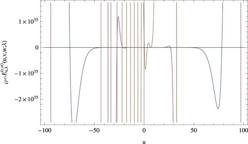
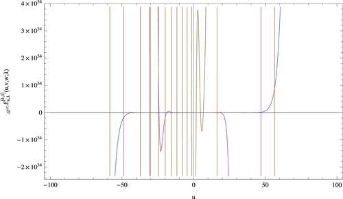
5.1. Computations related to ${}_{{\mathit{G}}^{\left(\sigma \right)}}{\mathcal{E}}_{\kappa }^{(c,\alpha )}(u,v,w;\lambda )$

Let us consider the first few members of ${}_{{\mathit{G}}^{\left(\sigma \right)}}{\mathcal{E}}_{\kappa }^{(c,\alpha )}(u,v,w;\lambda )$ which are given as: $\begin{array}{rl}& {}_{{\mathit{G}}^{\left(\sigma \right)}}{\mathcal{E}}_0^{(c,\alpha )}(u,v,w;\lambda )=\frac{16}{81},\\ & {}_{{\mathit{G}}^{\left(\sigma \right)}}{\mathcal{E}}_1^{(c,\alpha )}(u,v,w;\lambda )=-\frac{128}{243}+\frac{16u}{81},\\ & {}_{{\mathit{G}}^{\left(\sigma \right)}}{\mathcal{E}}_2^{(c,\alpha )}(u,v,w;\lambda )=\frac{896}{729}-\frac{256u}{243}+\frac{16u^2}{81}-\frac{16w^2}{81},\\ & {}_{{\mathit{G}}^{\left(\sigma \right)}}{\mathcal{E}}_3^{(c,\alpha )}(u,v,w;\lambda )=-\frac{1664}{729}+\frac{896u}{243}-\frac{128u^2}{81}+\frac{16u^3}{81}+\frac{32v}{27}+\frac{128w^2}{81}-\frac{16u{w}^2}{27},\\ & {}_{{\mathit{G}}^{\left(\sigma \right)}}{\mathcal{E}}_4^{(c,\alpha )}(u,v,w;\lambda )=\frac{5248}{2187}-\frac{6656u}{729}+\frac{1792u^2}{243}-\frac{512u^3}{243}+\frac{16u^4}{81}-\frac{1024v}{81}\\ & +\frac{128uv}{27}-\frac{1792w^2}{243}+\frac{512u{w}^2}{81}-\frac{32u^2{w}^2}{27}+\frac{16w^4}{81},\\ & {}_{{\mathit{G}}^{\left(\sigma \right)}}{\mathcal{E}}_5^{(c,\alpha )}(u,v,w;\lambda )=\frac{20864}{6561}+\frac{26240x}{2187}-\frac{16640x^2}{729}+\frac{8960x^3}{729}-\frac{640x^4}{243}+\frac{16x^5}{81}\\ & +\frac{17920v}{243}-\frac{5120xv}{81}+\frac{320x^{2}v}{27}+\frac{16640w^2}{729}-\frac{8960x{w}^2}{243}\\ & +\frac{1280x^2{w}^2}{81}-\frac{160x^3{w}^2}{81}-\frac{320v{w}^2}{27}-\frac{640w^4}{243}+\frac{80u{w}^4}{81}.\end{array}$ To show the shapes of the PKGHAEP ${}_{{\mathit{G}}^{\left(\sigma \right)}}{\mathcal{E}}_{\kappa }^{(c,\alpha )}(u,v,w;\lambda )$ for $\kappa =1,5,10,15,20,25,30$, $-100\le u\le 100$, v = 5, w = 6, $\sigma =3$, $\alpha =4$ and $\lambda =2$, Figure 1 is given.

Figure 1. Graph of the PKGHAEP ${}_{{\mathit{G}}^{\left(\sigma \right)}}{\mathcal{E}}_{\kappa }^{(c,\alpha )}(u,5,6;\lambda )$.

The results of numerical computations of real and complex zeros of the PKGHAEP ${}_{{\mathit{G}}^{\left(\sigma \right)}}{\mathcal{E}}_{\kappa }^{(c,\alpha )}(u,v,w;\lambda )$ for v = 5, w = 6 are mentioned in Table 3.

Table 3. Real and complex zeros of the PKGHAEP ${}_{{\mathit{G}}^{\left(3\right)}}{\mathcal{E}}_{\kappa }^{(c,4)}(u,5,6;2)$.

κ	Real zeros	Complex zeros
1	2.66667	–
2	$-3.40696,8.74029$	–
3	$-7.98745,2.94061,13.0468$	–
4	$-12.2585,0.304016,5.61458,17.0066$,	–
5	$-16.3761,-2.22546,4.26241,$	–
	6.79514, 20.8773
6	$-20.4056,-4.56172,1.98061,24.7206$	$7.13307-1.5258i,7.13307+1.5258i$
7	$-24.3802,-6.74644,-0.0745285,$	$8.13847-2.64017i,8.13847+2.64017i$
	5.03761, 28.5533
8	$-28.3184,-8.81144,-2.02027,$	$8.90755-3.77884i,8.90755+3.77884i,$
	$3.21645,7.07077,32.3811$
9	$-32.2315,-10.7794,-3.87898,1.45178,$	$9.63565-4.93371i,9.63565+4.93371i$
	$5.87933,8.08102,36.2064$
10	$-36.1264,-12.6672,-5.66131,$	$8.17674-0.690615i,8.17674+0.690615i,$
	$-0.273646,4.35813,40.0302$	$10.3267-6.08457i,10.3267+6.08457i$

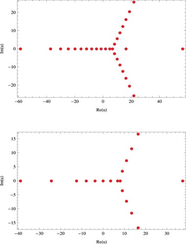
Next, we show certain beautiful zeros of ${}_{{\mathit{G}}^{\left(3\right)}}{\mathcal{E}}_{\kappa }^{(c,4)}(u,5,6;2)$ for $u\in \mathbb{C}$ in Figure 2.

Figure 2. Graphs of ${}_{{\mathit{G}}^{\left(3\right)}}{\mathcal{E}}_{30}^{(c,4)}(u,5,6;2)$ (top) and ${}_{{\mathit{G}}^{\left(3\right)}}{\mathcal{E}}_{20}^{(c,4)}(u,5,6;2)$ (bottom).

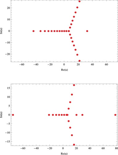
Remark 5.1

The PKGHAEP ${}_{{\mathit{G}}^{\left(\sigma \right)}}{\mathcal{E}}_{\kappa }^{(c,\alpha )}(u,a,b;\lambda )$, $u\in \mathbb{C}$, $a,b\in \mathbb{R}$ have $\mathrm{I}\mathrm{m}\left(u\right)=0$ reflection symmetry (Figure 2).

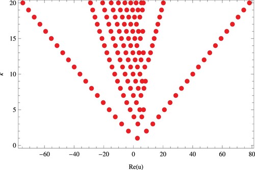
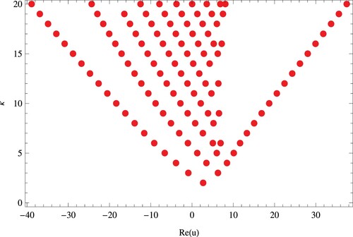
In Figure 3, we show the structure of real zeros of ${}_{{\mathit{G}}^{\left(3\right)}}{\mathcal{E}}_{\kappa }^{(c,4)}(u,5,6;2)$ for $1\le \kappa \le 20$.

Figure 3. Structure of real zeros of ${}_{{\mathit{G}}^{\left(3\right)}}{\mathcal{E}}_{\kappa }^{(c,4)}(u,5,6;2)$.

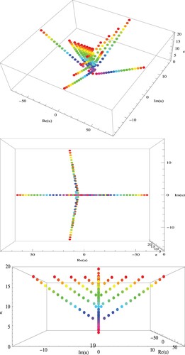
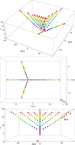
Figures 4, show the stacking structure of approximation zeros of the PKGHAEP ${}_{{\mathit{G}}^{\left(\sigma \right)}}{\mathcal{E}}_{\kappa }^{(c,\alpha )}(u,a,b;\lambda )=0$ for v = 5, w = 6, $\sigma =3$, $\alpha =4$, $\lambda =2$ and $1\le \kappa \le 20$.

Figure 4. Stacking structure zeros of ${}_{{\mathit{G}}^{\left(3\right)}}{\mathcal{E}}_{\kappa }^{(c,4)}(u,5,6;2)$.

5.2. Computations related to ${}_{{\mathit{G}}^{\left(\sigma \right)}}{\mathcal{E}}_{\kappa }^{(s,\alpha )}(u,v,w;\lambda )$

The first few members of ${}_{{\mathit{G}}^{\left(\sigma \right)}}{\mathcal{E}}_{\kappa }^{(s,\alpha )}(u,v,w;\lambda )$ are given as: $\begin{array}{rl}& {}_{{\mathit{G}}^{\left(\sigma \right)}}{\mathcal{E}}_0^{(s,\alpha )}(u,v,w;\lambda )=0,\\ & {}_{{\mathit{G}}^{\left(\sigma \right)}}{\mathcal{E}}_1^{(s,\alpha )}(u,v,w;\lambda )=0,\\ & {}_{{\mathit{G}}^{\left(\sigma \right)}}{\mathcal{E}}_2^{(s,\alpha )}(u,v,w;\lambda )=-\frac{256z}{243}+\frac{32xz}{81},\\ & {}_{{\mathit{G}}^{\left(\sigma \right)}}{\mathcal{E}}_3^{(s,\alpha )}(u,v,w;\lambda )=\frac{896z}{243}-\frac{256xz}{81}+\frac{16x^{2}z}{27}-\frac{16z^3}{81},\\ & {}_{{\mathit{G}}^{\left(\sigma \right)}}{\mathcal{E}}_4^{(s,\alpha )}(u,v,w;\lambda )=-\frac{6656z}{729}+\frac{3584xz}{243}-\frac{512x^{2}z}{81}+\frac{64x^{3}z}{81}+\frac{128yz}{27}\\ & +\frac{512z^3}{243}-\frac{64x{z}^3}{81},\\ & {}_{{\mathit{G}}^{\left(\sigma \right)}}{\mathcal{E}}_5^{(s,\alpha )}(u,v,w;\lambda )=\frac{26240z}{2187}-\frac{33280xz}{729}+\frac{8960x^{2}z}{243}-\frac{2560x^{3}z}{243}+\frac{80x^{4}z}{81}\\ & -\frac{5120yz}{81}+\frac{640xyz}{27}-\frac{8960z^3}{729}+\frac{2560x{z}^3}{243}-\frac{160x^2{z}^3}{81}+\frac{16z^5}{81}.\end{array}$ The 2D graphical representation of the PKGHAEP ${}_{{\mathit{G}}^{\left(\sigma \right)}}{\mathcal{E}}_{\kappa }^{(s,\alpha )}(u,v,w;\lambda )$ for $\kappa =1,5,10,15,20,25,30$, $-100\le u\le 100$, v = 5, w = 6, $\sigma =3$, $\alpha =4$ and $\lambda =2$, is shown in Figure 5.

Figure 5. Graph of the PKGHAEP ${}_{{\mathit{G}}^{\left(\sigma \right)}}{\mathcal{E}}_{\kappa }^{(c,\alpha )}(u,5,6;\lambda )$.

The approximate solutions satisfy the PKGHAEP ${}_{{\mathit{G}}^{\left(\sigma \right)}}{\mathcal{E}}_{\kappa }^{(s,\alpha )}(u,v,w;\lambda )=0$ when v = 5 and w = 6, are mentioned in Table 4.

Table 4. Real and complex zeros of the PKGHAEP ${}_{{\mathit{G}}^{\left(3\right)}}{\mathcal{E}}_{\kappa }^{(s,4)}(u,5,6;2)$.

κ	Real zeros	Complex zeros
1	–	–
2	2.66667	–
3	$-0.92344,6.25678$	–
4	$-3.9115,3.46326,8.44823$,	–
5	$-6.63887,1.24086,$	–
	5.97567, 10.089
6	$-9.18689,-1.02348,5.02073,$	–
	$6.90257,11.6204$
7	$-11.6082,-3.13291,$	$7.43057-2.07924i,7.43057+2.07924i$
	2.60609, 13.2739
8	$-13.9358,-5.13089,0.738042,$	$8.39279-3.43901i,8.39279+3.43901i,$
	$5.17584,15.0339$
9	$-16.192,-7.03508,-1.08619,$	$9.22078-4.75189i,9.22078+4.75189i$
	$3.85315,6.50744,16.8444$
10	$-18.3923,-8.85965,-2.83742,$	$6.65726-1.18058i,6.65726+1.18058i,$
	$2.08858,18.6803$	$10.003-6.00447i,10.003+6.00447i$

From Table 4, we remark that the PKGHAEP ${}_{{\mathit{G}}^{\left(\sigma \right)}}{\mathcal{E}}_{\kappa }^{(s,\alpha )}(u,v,w;\lambda )$ have $(\kappa -1)$ approximate solutions.

Certain interesting zeros of the PKGHAEP ${}_{{\mathit{G}}^{\left(3\right)}}{\mathcal{E}}_{\kappa }^{(c,4)}(u,5,6;2)$ for $u\in \mathbb{C}$ are shown in Figure 6.

Figure 6. Graphs of ${}_{{\mathit{G}}^{\left(3\right)}}{\mathcal{E}}_{30}^{(s,4)}(u,5,6;2)$ (top) and ${}_{{\mathit{G}}^{\left(3\right)}}{\mathcal{E}}_{20}^{(s,4)}(u,5,6;2)$ (bottom).

The structure of real zeros of ${}_{{\mathit{G}}^{\left(3\right)}}{\mathcal{E}}_{\kappa }^{(s,4)}(u,5,6;2)$ for $1\le \kappa \le 20$ is shown in Figure 7.

Figure 7. Structure of real zeros of ${}_{{\mathit{G}}^{\left(3\right)}}{\mathcal{E}}_{\kappa }^{(s,4)}(u,5,6;2)$.

The stacking structure of approximation zeros of the PKGHAEP ${}_{{\mathit{G}}^{\left(\sigma \right)}}{\mathcal{E}}_{\kappa }^{(s,\alpha )}(u,a,b;\lambda )=0$ when v = 5, w = 6, $\sigma =3$, $\alpha =4$, $\lambda =2$ and $1\le \kappa \le 20$ is shown in Figures 8.

Figure 8. Stacking structure zeros of ${}_{{\mathit{G}}^{\left(3\right)}}{\mathcal{E}}_{\kappa }^{(s,4)}(u,5,6;2)$.

6. Conclusions

In our current work, we introduced two parametric-hybrid classes of the Gould-Hopper-Eulerian-type polynomials. The properties of these classes are studied with the help of operational methods. Several useful formulae involving the parametric kind Gould-Hopper-Eulerian-type polynomials are derived. Certain significant special cases are also considered. The symmetric identities, integral equations related to these kinds of polynomials can be considered in further studies.

Acknowledgments

The author sincerely thank the editor and anonymous reviewers for their careful reviews and useful suggestions towards the improvement of the paper.

Disclosure statement

No potential conflict of interest was reported by the author(s).

References

- Gould HW, Hopper AT. Operational formulas connected with two generalizations of Hermite polynomials. Duke Math J. 1962;29:51–63.
- Khan S, Raza N. Determinantal approach to certain mixed special polynomials related to Gould–Hopper polynomial. Appl Math Comp. 2015;251:599–614.
- Bayad A, Kim T. Identities for Apostol-type Frobenius–Euler polynomials resulting from the study of a nonlinear operator. Russ J Math Phys. 2016;23:164–171.
- Masjed-Jamei M, Koepf W. Symbolic computation of some power-trigonometric series. Symb Comput. 2017;80:273–284.
- Dere R, Simsek Y, Srivastava HM. A unified presentation of three families of generalized Apostol type polynomials based upon the theory of the umbral calculus and the umbral algebra. J Number Theory. 2013;133:3245–3263.
- He Y, Araci S, Srivastava HM. Some new formulas for the products of the Apostol type polynomials. Adv Differ Equ. 2016;2016:1–18. (Article ID 287).
- He Y, Araci S, Srivastava HM, et al. Some new identities for the Apostol–Bernoulli polynomials and the Apostol–Genocchi polynomials. Appl Math Comput. 2015;262:31–41.
- Kim DS, Kim T, Lee H. A note on degenerate Euler and Bernoulli polynomials of complex variable. Symmetry. 2019;11(9):1–16. DOI:10.3390/sym11091168
- Luo Q-M. Apostol-Euler polynomials of higher order and Gaussian hypergeometric functions. Taiwanese J Math. 2006;10:917–925.
- Luo Q-M. Extensions of the Genocchi polynomials and their Fourier expansions and integral representations. Osaka J Math. 2011;48:291–309.
- Luo Q-M, Srivastava HM. Some generalizations of the Apostol–Bernoulli and Apostol–Euler polynomials. J Math Anal Appl. 2005;308:290–302.
- Lu D-Q, Srivastava HM. Some series identities involving the generalized Apostol type and related polynomials. Comput Math Appl. 2011;62:3591–3602.
- Masjed-Jamei M, Beyki MR, Koepf W. A new type of Euler polynomials and numbers. Mediterr J Math. 2018;15(138):1–17.
- Yasmin G, Muhyi A. Certain results of 2-variable q-generalized tangent-Apostol type polynomials. J Math Comput Sci. 2020;22:238–251.
- Srivastava HM, Kızılate C. A parametric kind of the Fubini-type polynomials. RACSAM Rev R Acad Cienc Exactas Fís Nat Ser A Mat. 2019;113:3253–3267.
- Srivastava HM, Masjed-Jamei M, Beyki MR. A parametric type of the Apostol–Bernoulli, Apostol–Euler and Apostol–Genocchi polynomials. Appl Math Inform Sci. 2018;12:907–916.
- Kilar N, Simsek Y. Two parametric kinds of Eulerian-type polynomials associated with Euler's formula. Symmetry. 2019;11:1–19. DOI:10.3390/sym11091097
- Cocolicchio D, Dattoli G, Srivastava HM, editors. Advanced special functions and applications. Proceedings of the First Melfi School on Advanced Topics in Mathematics and Physics. Rome: Aracne Editrice; 2000.
- Khan S, Raza N, Ali M. Finding mixed families of special polynomials associated with Appell sequences. J Math Anal Appl. 2017;447(1):398–418.
- Muhyi A, Araci S. A note on q-Fubini-Appell polynomials and related properties. J Funct Spaces. 2021;2021:1–9. DOI:10.1155/2021/3805809.
- Srivastava HM, Özarslan MA, Yılmaz B. Some families of differential equations associated with the Hermite-based Appell polynomials and other classes of Hermite-based polynomials. Filomat. 2014;28(4):695–708.
- Srivastava HM, Araci S, Khan WA, et al. A note on the truncated-exponential based Apostol-type polynomials. Symmetry. 2019;11(4):1–20. DOI:10.3390/sym11040538
- Srivastava HM, Srivastava R, Muhyi A, et al. Construction of a new family of Fubini-type polynomials and its applications. Adv Difference Equ. 2021;2021(1):1–25.
- Yasmin G, Muhyi A. Certain results of hybrid families of special polynomials associated with Appell sequences. Filomat. 2019;33(12):3833–3844.
- Yasmin G, Muhyi A. Extended forms of Legendre-Gould-Hopper-Appell polynomials. Adv Stud Contemp Math. 2019;29(4):489–504.