Conjugate gradient method for simultaneous identification of the source term and initial data in a time-fractional diffusion equation

ABSTRACT

In this paper, we consider the simultaneous inversion of the source term and the initial data for a time-fractional diffusion equation based on the additional temperatures at two fixed times $t=T_1$ and $t=T_2$. The inverse problem is formulated on the basis of the Fourier method as an operator equation of the first kind. For the overdetermined system of linear equations, we apply the conjugate gradient method with an appropriate stopping criterion to solve the least-squares problems. The method is not only able to converge quickly, but also it can solve large-scale linear equations. Based on the proposed results, it can be seen that the iteration numbers play a role of a regularization parameter. Four numerical examples are provided to demonstrate the effectiveness of the proposed method.

KEYWORDS:

• Ill-posedness
• stopping criterion
• conditional stability
• minimization functional
• iteration method

AMS Subject Classifications:

• 65N21
• 47A52
• 35R30

1. Introduction

Many time-fractional diffusion equations and diffusion wave equations appear when the standard time derivatives are replaced by the time-fractional derivatives. Sub-diffusion $(0<\alpha <1)$ and super-diffusion phenomena $(1<\alpha <2)$ can be described by the fractional equations [1, 2]. Fractional diffusion equations (FDEs) play an important role in describing asymmetric phenomena. Because it can better fit some natural physical process and dynamic systems, the kind of equations have received a lot of attentions in recent years, such as [3–9].

The fractional calculus is an important tool in the field of applied mathematics to solve the real-world problems, due to its applicability in the different areas of science and engineering. FDEs have an advantage in modelling of real-life phenomena because it will reduce the errors arising from the ignored parameters. Moreover, the most interesting one is that the data fitting can be considered better with fractional order rather than integer-order. In recent years, there are many papers to study the real-life phenomena, see for [10–14]. More recently, new fractional operators play an important role to model a variety of natural phenomena and processes, such as [15–19].

However, for some practical situations, it is difficult to measure some parameters directly and it needs to obtain by some skilled method indirectly. The inverse problems of the source term and the initial data in the time-fractional diffusion equations have been studied extensively in recent years, and one can refer to [20–27].

Let $\mathrm{\Omega }\subset {\mathbb{R}}^n$ be an open bounded domain with sufficiently smooth boundary $\mathrm{\partial }\mathrm{\Omega }$. We consider the following time-fractional diffusion equation with homogeneous Dirichlet boundary condition: (1) $\{\begin{array}{ll}{\displaystyle \frac{{\mathrm{\partial }}^{\alpha }u(x,t)}{\mathrm{\partial }{t}^{\alpha }}}+Lu(x,t)=f\left(x\right),& (x,t)\in \mathrm{\Omega }\times (0,T),\\ u(x,t)=0,& (x,t)\in \mathrm{\partial }\mathrm{\Omega }\times (0,T),\\ u(x,0)=u^0\left(x\right),& x\in \mathrm{\Omega },\end{array}$(1) where $0<\alpha <1$, and L is a symmetric strongly elliptic operator defined by $L\left(u\right)=-\sum _{i=1}^n\frac{\mathrm{\partial }}{\mathrm{\partial }{x}_i}\left(\sum _{j=1}^n{\theta }_{i,j}\right(x\left)\frac{\mathrm{\partial }}{\mathrm{\partial }{x}_j}u\right(x\left)\right)+c\left(x\right)u\left(x\right),$ in which ${\theta }_{i,j}\left(x\right)$ and $c\left(x\right)$ are sufficiently smooth functions on $\overline{\mathrm{\Omega }}$ satisfying ${\theta }_{i,j}\left(x\right)\in C^1\left(\overline{\mathrm{\Omega }}\right),{\theta }_{i,j}\left(x\right)={\theta }_{j,i}\left(x\right),c\left(x\right)\in C\left(\overline{\mathrm{\Omega }}\right),c\left(x\right)\ge 0,\mathrm{\forall }x\in \overline{\mathrm{\Omega }},$ and there is a constant v>0 such that $v\sum _{i=1}^n{\xi }_i^2\le \sum _{i,j=1}^n{\theta }_{i,j}\left(x\right){\xi }_i{\xi }_j$, $\mathrm{\forall }x\in \overline{\mathrm{\Omega }}$, $\xi \in {\mathbb{R}}^n$. Moreover, ${\mathrm{\partial }}^{\alpha }u(x,t)/\mathrm{\partial }{t}^{\alpha }$ is the Caputo fractional derivative of order α defined by (2) $\frac{{\mathrm{\partial }}^{\alpha }u(x,t)}{\mathrm{\partial }{t}^{\alpha }}=\frac{1}{\mathrm{\Gamma }(1-\alpha )}{\int }_0^t(t-\eta {)}^{-\alpha }\frac{\mathrm{\partial }u}{\mathrm{\partial }\eta }\mathrm{d}\eta ,0<\alpha <1,$(2) where $\mathrm{\Gamma }(\cdot )$ is the Gamma function.

Remark 1.1

Generally speaking, the source term is usually assumed as $R(x,t)f\left(x\right)$, where $R(x,t)$ is known in advance. However, for the sake of simplicity, we only consider the case that $R(x,t)\equiv 1$, i.e. the source item is only dependent of x.

As we know, if the source term $f\left(x\right)$ in (1(1) $\{\begin{array}{ll}{\displaystyle \frac{{\mathrm{\partial }}^{\alpha }u(x,t)}{\mathrm{\partial }{t}^{\alpha }}}+Lu(x,t)=f\left(x\right),& (x,t)\in \mathrm{\Omega }\times (0,T),\\ u(x,t)=0,& (x,t)\in \mathrm{\partial }\mathrm{\Omega }\times (0,T),\\ u(x,0)=u^0\left(x\right),& x\in \mathrm{\Omega },\end{array}$(1) ) is given, the identification of the initial data $u^0\left(x\right)$ from the final time temperature is severally ill-posed. This kind of inverse problem has been studied extensively. In [28], authors applied a non-local boundary value problem method to restore the initial value. In [29], Oanh used the conjugate gradient method to approximate the initial value. On the other hand, the identification problem of the source is also an ill-posed problem. In [30], authors studied an inverse time-dependent source problem from an additional integration condition. In [31], Yan et al. used an adjoint problem approach to determine the space-dependent source term in a time-fractional diffusion equation. Some theoretical discussions on uniqueness and existence results have been investigated in [32]. And in [33], Li et al. reconstructed a time-dependent source term in a multi-term time-fractional diffusion equation from the boundary Cauchy data. In [34], authors applied the Tikhonov regularization method to inverse the source term for the time-fractional heat equation in the view of the ABC-fractional technique. Wang et al. in [35] considered the simultaneous identification of the initial field and spatial heat source for the heat conduction process from extra measurements with the two additional measurement data at different times.

In recent years, inspired by some practical applications, several researchers begin to reconstruct the source and initial distribution simultaneously from the additional measured data, such as [36, 37]. Usually, the simultaneous recovery of the source term and the initial data is hard to be realized. In [36], Ruan et al. gave the conditional stability results and applied the Tikhonov regularization method to determine the source term and the initial data simultaneously. In [37], authors used a Landweber iteration method to solve the same problem by a priori and a posteriori parameter choice rules. This proposed paper considers a general conjugate gradient method to solve the same problem above. That is to say, we need not to deal with the adjoint and sensitive problem in this paper.

Based on the existence and conditional stability of the weak solution to (1(1) $\{\begin{array}{ll}{\displaystyle \frac{{\mathrm{\partial }}^{\alpha }u(x,t)}{\mathrm{\partial }{t}^{\alpha }}}+Lu(x,t)=f\left(x\right),& (x,t)\in \mathrm{\Omega }\times (0,T),\\ u(x,t)=0,& (x,t)\in \mathrm{\partial }\mathrm{\Omega }\times (0,T),\\ u(x,0)=u^0\left(x\right),& x\in \mathrm{\Omega },\end{array}$(1) ), we firstly apply the Fourier series expansion method to solve the direct problem in this paper. Secondly, we transform the inverse problem into a linear equation Ax = b. That is, when the problem (1(1) $\{\begin{array}{ll}{\displaystyle \frac{{\mathrm{\partial }}^{\alpha }u(x,t)}{\mathrm{\partial }{t}^{\alpha }}}+Lu(x,t)=f\left(x\right),& (x,t)\in \mathrm{\Omega }\times (0,T),\\ u(x,t)=0,& (x,t)\in \mathrm{\partial }\mathrm{\Omega }\times (0,T),\\ u(x,0)=u^0\left(x\right),& x\in \mathrm{\Omega },\end{array}$(1) ) is solvable, the kth iterate $x_k$ minimizes the error $x-x_k$ in the so-called energy norm $(x-x_k,A(x-x_k\left)\right)$. Then we apply the general conjugate gradient method with an appropriate stopping criterion, in which one can refer to [38, 39], to solve the linear equation from the measured temperatures with $t=T_1$ and $t=T_2$ $(0<T_1<T_2)$.

The remainder of this paper is organized as follows. In Section 2, we present some preliminaries for the inverse problem. Then we formulate the direct problem as a linear equation and give the conditional stability for the inverse problem in Section 3. In Section 4, we present the conjugate gradient algorithm. Numerical results for four different examples are provided in Section 5. In Section 6, we give a brief conclusion.

2. Preliminaries

In this section, we derive the solution of the problem (1(1) $\{\begin{array}{ll}{\displaystyle \frac{{\mathrm{\partial }}^{\alpha }u(x,t)}{\mathrm{\partial }{t}^{\alpha }}}+Lu(x,t)=f\left(x\right),& (x,t)\in \mathrm{\Omega }\times (0,T),\\ u(x,t)=0,& (x,t)\in \mathrm{\partial }\mathrm{\Omega }\times (0,T),\\ u(x,0)=u^0\left(x\right),& x\in \mathrm{\Omega },\end{array}$(1) ) based on the eigenfunction of L and give some definitions and lemmas which can be used in latter sections [40].

Definition 2.1

The Mittag-Leffler function is defined by $E_{a,b}\left(z\right)=\sum _{k=0}^{\mathrm{\infty }}\frac{z^k}{\mathrm{\Gamma }(ak+b)},z\in \mathbb{C},$ where arbitrary constants a>0 and $b\in \mathbb{R}$.

Lemma 2.1

(a)	For $0<\alpha <1$ and $\eta >0$, $0\le E_{\alpha ,1}(-\eta )<1,\frac{{\mathrm{d}}^{\alpha }}{\mathrm{d}{\eta }^{\alpha }}{E}_{\alpha ,1}(-\lambda {\eta }^{\alpha })=-\lambda E_{\alpha ,1}(-\lambda {\eta }^{\alpha }).$ In addition, $E_{\alpha ,1}(-\eta )$ is fully monotonic. That is to say, $(-1{)}^n{\mathrm{d}}^n{E}_{\alpha ,1}(-\eta )/\mathrm{d}{\eta }^n\ge$ 0. When $\eta \to +\mathrm{\infty }$, $E_{\alpha ,1}(-\eta )$ satisfies the following approximation relation: $E_{\alpha ,1}(-\eta )=\frac{1}{\eta \mathrm{\Gamma }(1-\alpha )}+o(\mid \eta {\mid }^{-2}).$
(b)	For $\lambda >0$, $\alpha >0$ and positive integer $m\in \mathbb{N}$, $\frac{{\mathrm{d}}^m}{\mathrm{d}{t}^m}{E}_{\alpha ,1}(-\lambda t^{\alpha })=-\lambda t^{\alpha -1}{E}_{\alpha ,\alpha -m+1}(-\lambda t^{\alpha }),t>0.$
(c)	Suppose that $0<{\alpha }_0<{\alpha }_1<1$. Then there exists constants c, C>0, which only has something to do with ${\alpha }_0$ and ${\alpha }_1$, such that $\frac{c}{\mathrm{\Gamma }(1-\alpha )}\frac{1}{1-t}\le E_{\alpha ,1}\left(t\right)\le \frac{C}{\mathrm{\Gamma }(1-\alpha )}\frac{1}{1-t},\mathrm{\forall }t<0$ uniformly for all $\alpha \in [{\alpha }_0,{\alpha }_1]$.

While $u^0\left(x\right)$ and $f\left(x\right)$ are unknown functions, the problem of restoring source term and initial temperature distribution is underdetermined and additional data must be given. In this paper, the additional temperature measurements are (3) $u(x,T_1)\approx g_1^{\delta }\left(x\right),u(x,T_2)\approx g_2^{\delta }\left(x\right).$(3) So the main idea of the paper is to determine the source term and the initial temperature simultaneously from $g_1^{\delta }\left(x\right)$ and $g_2^{\delta }\left(x\right)$. Because of the linearity of the problem (1(1) $\{\begin{array}{ll}{\displaystyle \frac{{\mathrm{\partial }}^{\alpha }u(x,t)}{\mathrm{\partial }{t}^{\alpha }}}+Lu(x,t)=f\left(x\right),& (x,t)\in \mathrm{\Omega }\times (0,T),\\ u(x,t)=0,& (x,t)\in \mathrm{\partial }\mathrm{\Omega }\times (0,T),\\ u(x,0)=u^0\left(x\right),& x\in \mathrm{\Omega },\end{array}$(1) ), it can be divided into two sub-problems: (4) $\{\begin{array}{ll}{\displaystyle \frac{{\mathrm{\partial }}^{\alpha }{u}_1(x,t)}{\mathrm{\partial }{t}^{\alpha }}}+L{u}_1(x,t)=f\left(x\right),& (x,t)\in \mathrm{\Omega }\times (0,T),\\ u_1(x,t){\mid }_{\mathrm{\partial }\mathrm{\Omega }}=0,& (x,t)\in \mathrm{\partial }\mathrm{\Omega }\times (0,T),\\ u_1(x,t){\mid }_{t=0}=0,& x\in \mathrm{\Omega },\end{array}$(4) and (5) $\{\begin{array}{ll}{\displaystyle \frac{{\mathrm{\partial }}^{\alpha }{u}_2(x,t)}{\mathrm{\partial }{t}^{\alpha }}}+L{u}_2(x,t)=0,& (x,t)\in \mathrm{\Omega }\times (0,T),\\ u_2(x,t){\mid }_{\mathrm{\partial }\mathrm{\Omega }}=0,& (x,t)\in \mathrm{\partial }\mathrm{\Omega }\times (0,T),\\ u_2(x,t){\mid }_{t=0}=u^0\left(x\right),& x\in \mathrm{\Omega },\end{array}$(5) such that (6) $u(x,t)=u_1(x,t)+u_2(x,t).$(6)

3. Conditional stability for the inverse problem

Denote the eigenvalues of the operator L as ${\lambda }_n\in \mathbb{R}$ and corresponding orthonormal eigenfunctions as ${\phi }_n\left(x\right)\in H^2\left(\mathrm{\Omega }\right)\bigcap H_0^1\left(\mathrm{\Omega }\right)$, which means $L{\phi }_n={\lambda }_n{\phi }_n$, counting according to the multiplicities, we note $0<{\lambda }_1\le {\lambda }_2\le \cdots \le {\lambda }_n\le \cdots ,\underset{n\to \mathrm{\infty }}{lim}{\lambda }_n=+\mathrm{\infty },$ and sequence $\{{\phi }_n{\}}_{n\in \mathbb{N}}$ is orthonomal basis in $L^2\left(\mathrm{\Omega }\right)$. Define (7) $D\left(\right(L{)}^{\theta })=\{\chi \in L^2(\mathrm{\Omega }):{(\sum _{n=1}^{+\mathrm{\infty }}{\lambda }_n^{2\theta }\mid 〈\chi ,{\phi }_n〉{\mid }^2)}^{\frac{1}{2}}<\mathrm{\infty }\},$(7) where $〈\cdot ,\cdot 〉$ denotes its inner product in $L^2\left(\mathrm{\Omega }\right)$. It is easy to get that $D\left(\right(L{)}^{\theta })$ is a Hilbert space with the norm $\Vert \chi {\Vert }_{D\left(\right(L{)}^{\theta })}=(\sum _{n=1}^{\mathrm{\infty }}{\lambda }_n^{2\theta }|〈\chi ,{\phi }_n〉{|}^2{)}^{\frac{1}{2}}$ (see [32]). By the method of separation of variables and Lemma 2.1, we know that the formal solutions of (4(4) $\{\begin{array}{ll}{\displaystyle \frac{{\mathrm{\partial }}^{\alpha }{u}_1(x,t)}{\mathrm{\partial }{t}^{\alpha }}}+L{u}_1(x,t)=f\left(x\right),& (x,t)\in \mathrm{\Omega }\times (0,T),\\ u_1(x,t){\mid }_{\mathrm{\partial }\mathrm{\Omega }}=0,& (x,t)\in \mathrm{\partial }\mathrm{\Omega }\times (0,T),\\ u_1(x,t){\mid }_{t=0}=0,& x\in \mathrm{\Omega },\end{array}$(4) ) and (5(5) $\{\begin{array}{ll}{\displaystyle \frac{{\mathrm{\partial }}^{\alpha }{u}_2(x,t)}{\mathrm{\partial }{t}^{\alpha }}}+L{u}_2(x,t)=0,& (x,t)\in \mathrm{\Omega }\times (0,T),\\ u_2(x,t){\mid }_{\mathrm{\partial }\mathrm{\Omega }}=0,& (x,t)\in \mathrm{\partial }\mathrm{\Omega }\times (0,T),\\ u_2(x,t){\mid }_{t=0}=u^0\left(x\right),& x\in \mathrm{\Omega },\end{array}$(5) ) are given by (8) $\begin{array}{rl}{u}_1(x,t)& =\sum _{n=1}^{+\mathrm{\infty }}{f}_n\frac{1-E_{\alpha ,1}(-{\lambda }_n{t}^{\alpha })}{{\lambda }_n}{\phi }_n\left(x\right),\end{array}$(8) (9) $\begin{array}{rl}{u}_2(x,t)& =\sum _{n=1}^{+\mathrm{\infty }}{E}_{\alpha ,1}(-{\lambda }_n{t}^{\alpha })u_n^0{\phi }_n\left(x\right),\end{array}$(9) where $f_n=(f,{\phi }_n)$, $u_n^0=(u^0,{\phi }_n)$, $n=1,2,\cdots$.

Let $t=T_i,i=1,2$, we can define four linear operators according to the problems (4(4) $\{\begin{array}{ll}{\displaystyle \frac{{\mathrm{\partial }}^{\alpha }{u}_1(x,t)}{\mathrm{\partial }{t}^{\alpha }}}+L{u}_1(x,t)=f\left(x\right),& (x,t)\in \mathrm{\Omega }\times (0,T),\\ u_1(x,t){\mid }_{\mathrm{\partial }\mathrm{\Omega }}=0,& (x,t)\in \mathrm{\partial }\mathrm{\Omega }\times (0,T),\\ u_1(x,t){\mid }_{t=0}=0,& x\in \mathrm{\Omega },\end{array}$(4) ) and (5(5) $\{\begin{array}{ll}{\displaystyle \frac{{\mathrm{\partial }}^{\alpha }{u}_2(x,t)}{\mathrm{\partial }{t}^{\alpha }}}+L{u}_2(x,t)=0,& (x,t)\in \mathrm{\Omega }\times (0,T),\\ u_2(x,t){\mid }_{\mathrm{\partial }\mathrm{\Omega }}=0,& (x,t)\in \mathrm{\partial }\mathrm{\Omega }\times (0,T),\\ u_2(x,t){\mid }_{t=0}=u^0\left(x\right),& x\in \mathrm{\Omega },\end{array}$(5) ) as following $\begin{array}{r}{K}_{1,i}:f\mapsto u_1(x,T_i),i=1,2,\\ K_{2,i}:u^0\mapsto u_2(x,T_i),i=1,2.\end{array}$ In order to restore $u^0\left(x\right)$ and $f\left(x\right)$ simultaneously, we obtain two expressions of operator equations (10) $\begin{array}{rl}& \left(K_{1,1}\right(f\left)\right)\left(x\right)+\left(K_{2,1}\right(u^0\left)\right)\left(x\right)=g_1\left(x\right),\end{array}$(10) (11) $\begin{array}{rl}& \left(K_{1,2}\right(f\left)\right)\left(x\right)+\left(K_{2,2}\right(u^0\left)\right)\left(x\right)=g_2\left(x\right),\end{array}$(11) which can be written in the matrix form (12) $A\left(\begin{array}{c}f\\ u^0\end{array}\right)=\left(\begin{array}{c}{g}_1\\ g_2\end{array}\right),\mathrm{w}\mathrm{h}\mathrm{e}\mathrm{r}\mathrm{e}A=\left(\begin{array}{cc}{K}_{1,1}& K_{2,1}\\ K_{1,2}& K_{2,2}\end{array}\right),$(12) and by analysis we know the adjoint operator of A $A^{\ast }=\left(\begin{array}{cc}{K}_{1,1}^{\ast }& K_{1,2}^{\ast }\\ K_{2,1}^{\ast }& K_{2,2}^{\ast }\end{array}\right).$

Theorem 3.1

Define $g_i=u(\cdot ,T_i)$ for i = 1, 2. If $f\left(x\right)$ and $u^0\left(x\right)\in D\left(\right(L{)}^{\theta })$ satisfy the a priori bound condition (13) $max\left\{\Vert f\left(x\right){\Vert }_{D\left(\right(L{)}^{\theta })},\Vert u^0\left(x\right){\Vert }_{D\left(\right(L{)}^{\theta })}\right\}\le E,$(13) then we have $\begin{array}{rl}\Vert f\Vert & \le C{E}^{\frac{1}{\theta +1}}(\Vert g_1\Vert +{\left(\frac{T_2}{T_1}\right)}^{\alpha }\Vert g_2\Vert {)}^{\frac{\theta }{\theta +1}},\Vert u^0\Vert \\ & \le C{E}^{\frac{1}{\theta +1}}{(\frac{1}{1-E_{\alpha ,1}(-{\lambda }_1{T}_1^{\alpha })}\Vert g_1\Vert +\Vert g_2\Vert )}^{\frac{\theta }{\theta +1}},\end{array}$ in which θ is a positive constant.

A proof can be found in [36].

4. The conjugate gradient regularization method

From the above theorem, we known that the simultaneous inversion of the initial data and the source term is ill-posed, the corresponding minimization problem is also unstable, that is to say, a small perturbation in the data may cause dramatically large errors in the numerical solution. Therefore, the regularization method is essential to restore the stability of the problem. In this paper, we employ the conjugate gradient method with an appropriate stopping rule to solve the problem.

The conjugate gradient algorithm can be considered a minimization problem (14) $J\left(x\right)=\frac{1}{2}\Vert Ax-b{\Vert }^2,$(14) where A is an $n\times n$ matrix(or an operator on a Hilbert space), x and b are vectors, that is, $n\times 1$ matrices. And if A is a self-adjoint and positive definite, the minimizer of this function satisfies equation Ax = b. So it is a significant method to solve linear equations. It is characterized by the property of stepping at each iteration in the direction of the component of the gradient A-conjugate to the preceding step direction, and by the property of finite termination under exact arithmetic. The residual at step m can be expressed as (15) $R=A{x}_m-b,$(15) where the initial residual $R_0=A{x}_0-b$, and thus the distribution of eigenvalues is employed. The method will converge in m or fewer iterations if the operator has k distinct eigenvalues. For simplicity, we take the initial guess $x_0=0$, giving an initial residual or negative gradient of $r_0=-A^{\ast }b$, and it can be taken as our first step direction $p_0$ as well.

The concrete process of the algorithm is as follows:

Step 1. Choose $\left(\begin{array}{c}f\\ u^0\end{array}\right)=\left(\begin{array}{c}{f}_{initial}\\ u_{initial}^0\end{array}\right),$ and set $m=0.$

Step 2. Calculate the initial search direction $p^0=-A^{\ast }\left(\begin{array}{c}{g}_1\\ g_2\end{array}\right).$

Step 3. Solve the direct problem (1(1) $\{\begin{array}{ll}{\displaystyle \frac{{\mathrm{\partial }}^{\alpha }u(x,t)}{\mathrm{\partial }{t}^{\alpha }}}+Lu(x,t)=f\left(x\right),& (x,t)\in \mathrm{\Omega }\times (0,T),\\ u(x,t)=0,& (x,t)\in \mathrm{\partial }\mathrm{\Omega }\times (0,T),\\ u(x,0)=u^0\left(x\right),& x\in \mathrm{\Omega },\end{array}$(1) ) with $\left(\begin{array}{c}f\\ u^0\end{array}\right)=\left(\begin{array}{c}{f}_m\\ u_m^0\end{array}\right),$ and determine the residual $R_m=A\left(\begin{array}{c}{f}_m\\ u_m^0\end{array}\right)-\left(\begin{array}{c}{g}_1\\ g_2\end{array}\right),$ and $r_m=A^{\ast }(A\left(\begin{array}{c}{f}_m\\ u_m^0\end{array}\right)-\left(\begin{array}{c}{g}_1\\ g_2\end{array}\right)).$

Step 4. Determine the search direction $p^m=r_m+{\gamma }_{m-1}{p}^{m-1},$ and ${\gamma }_m=\frac{\Vert r_m{\Vert }^2}{\Vert r_{m-1}{\Vert }^2},$ for  $m\ge 1$.

Step 5. Solve $u_m$ for the problem (1(1) $\{\begin{array}{ll}{\displaystyle \frac{{\mathrm{\partial }}^{\alpha }u(x,t)}{\mathrm{\partial }{t}^{\alpha }}}+Lu(x,t)=f\left(x\right),& (x,t)\in \mathrm{\Omega }\times (0,T),\\ u(x,t)=0,& (x,t)\in \mathrm{\partial }\mathrm{\Omega }\times (0,T),\\ u(x,0)=u^0\left(x\right),& x\in \mathrm{\Omega },\end{array}$(1) ) with $\left(\begin{array}{c}f\\ u^0\end{array}\right)=p^{m}and\left(\begin{array}{c}{g}_1\\ g_2\end{array}\right)=\left(\begin{array}{c}0\\ 0\end{array}\right).$ Set $t_m=\frac{(R_m,A{p}^m)}{\Vert A{p}^m{\Vert }^2},$ and we let $\left(\begin{array}{c}{f}_{m+1}\\ u_{m+1}^0\end{array}\right)=\left(\begin{array}{c}{f}_m\\ u_m^0\end{array}\right)-t_m{p}^m.$

Step 6. Increase m by one and go to Step 3.

If $r_m=0$, the iteration procedure is stopped, and we suppose $\left(\begin{array}{c}{f}_k\\ u_k^0\end{array}\right)=\left(\begin{array}{c}{f}_m\\ u_m^0\end{array}\right)$ for $k\ge m$. For the above iteration algorithm, a suitable stopping rule is essential to get the precise and stable solution of the inverse problem. So we choose the first m such that $\Vert r_m{\Vert }_{L^2\left(\mathrm{\Omega }\right)}\le \tau \delta ,$ where $\tau >1$ is a constant and can be taken heuristically to be 1.01 as suggested by Hanke and Hansen [41]. If the noise level tends to zero, the iteration procedure converges to the exact solution for Example 5.1.

5. Numerical results and discussion

In this section, we show four numerical examples to illustrate the effectiveness of the proposed algorithm.

The noisy data are generated by adding random perturbations to test the stability of the algorithm, i.e. (16) $g_1^{\delta }=g_1+g_1\ast \delta \ast \left[2randn\right(size\left(g_1\right))-1],g_2^{\delta }=g_2+g_2\ast \delta \ast \left[2randn\right(size\left(g_2\right))-1],$(16) where δ is noisy level which is calculated by $\Vert u(x,T_1)-g_1^{\delta }\left(x\right){\Vert }_{L^2\left(\mathrm{\Omega }\right)}\le \delta ,\Vert u(x,T_2)-g_2^{\delta }\left(x\right){\Vert }_{L^2\left(\mathrm{\Omega }\right)}\le \delta$, and Matlab function $randn(\cdot )$ generates random numbers uniformly distributed on [0,1]. In order to test the accuracy of the above method, we calculate the relative errors defined by (17) ${ϵ}_f=\frac{\Vert f\left(x\right)-f_m^{\delta }\left(x\right){\Vert }_{L^2\left(\mathrm{\Omega }\right)}}{\Vert f\left(x\right){\Vert }_{L^2\left(\mathrm{\Omega }\right)}},$(17) and (18) ${ϵ}_{u^0}=\frac{\Vert u^0\left(x\right)-u_m^{0,\delta }\left(x\right){\Vert }_{L^2\left(\mathrm{\Omega }\right)}}{\Vert u^0\left(x\right){\Vert }_{L^2\left(\mathrm{\Omega }\right)}},$(18) where m is the iteration number, and δ is the noisy level.

Example 5.1

Consider the example with the exact solution $u(x,t)=E_{1/2,1}(-{\pi }^2{t}^{1/2})\sin \left(\pi x\right)+E_{1/2,1}(-4{\pi }^2{t}^{1/2})\sin \left(2\pi x\right)-\frac{\sin \left(\pi x\right)}{{\pi }^2},$ its smooth heat source is given by the sine function (19) $f\left(x\right)=-\sin \left(\pi x\right),$(19) and the initial value is given by (20) $u^0\left(x\right)=\sin \left(2\pi x\right)+\frac{{\pi }^2-1}{{\pi }^2}\sin \left(\pi x\right).$(20) The reconstructed solutions are shown in Figure 1, in which satisfactory approximated solutions with $\delta =0\mathrm{\%}$, $\delta =0.01\mathrm{\%}$ and $\delta =0.1\mathrm{\%}$ are obtained respectively. We can observe from Figures 1 and 2 that the source term and the initial value are only mildly effected by the data errors. The relative $L^2$-norm error ε for different noisy level δ is given in Table 1.

Figure 1. Numerical results for initial value and source term in Example 1. (a) Source term with $T_1=0.2$ $T_2=0.5$, n = 4. (b) Initial data with $T_1=0.2$ $T_2=0.5$, n = 4.

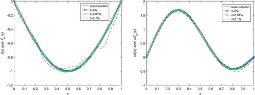
Figure 2. Numerical results for initial value and source term in Example 5.2. (a) Source term with $\alpha =0.3$ $T_1=0.2$, $T_2=0.5$. (b) Initial value with $\alpha =0.3$ $T_1=0.2$, $T_2=0.5$.

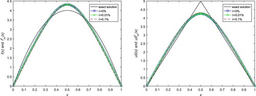
Table 1. The relative errors and the stop steps of $f\left(x\right)$, $u^0\left(x\right)$ with different noisy level δ for Example 5.1.

$ϵ╲\delta$	$\delta =0$	$\delta =0.01\mathrm{\%}$	$\delta =0.1\mathrm{\%}$
${ϵ}_f$	$1.3633\times {10}^{-11}\left(4\right)$	$1.6\times {10}^{-2}\left(4\right)$	$8.77\times {10}^{-2}\left(4\right)$
${ϵ}_{u^0}$	$1.1740\times {10}^{-11}\left(4\right)$	$1.32\times {10}^{-2}\left(4\right)$	$5.91\times {10}^{-2}\left(4\right)$

Example 5.2

Consider the smooth heat source (21) $f\left(x\right)=16x(1-x),$(21) and the piecewise smooth initial value (22) $u^0\left(x\right)=\{\begin{array}{ll}10x,& 0\le x<{\displaystyle \frac{1}{2}},\\ 10(1-x),& {\displaystyle \frac{1}{2}}\le x\le 1.\end{array}$(22) In this example, the initial value is not smooth, so we calculate a formal solution by Fourier series as follows: $\begin{array}{rl}u(x,t)& =\sum _{k=1}^{\mathrm{\infty }}\left[{\int }_0^{1}16x\right(1-x)\sin (k\pi x)\mathrm{d}x\frac{1-E_{\alpha ,1}(-{\lambda }_k{t}^{\alpha })}{{\lambda }_k}\\ & +E_{\alpha ,1}(-{\lambda }_k{t}^{\alpha }){\int }_0^1{u}^0\left(x\right)\sin \left(k\pi x\right)\mathrm{d}x]\sin \left(k\pi x\right).\end{array}$ The heat source term is a quadratic function and the initial value is a continuous but not differentiable function. It is easy to see that there is a sharp point at $x=1/2$, which is usually very difficult to be reconstructed because of the lower regularity.

The exact solution and the numerical ones are given in Figures 2 and 3 in the case of $\alpha =0.3$, 0.9 respectively. We find that the relative error of $f\left(x\right)$ becomes smaller as the increase of α, but the one of $u^0\left(x\right)$ becomes bigger. That is to say, the reconstruction of initial data is more difficult than the source term.

Figure 3. Numerical results for initial value and source term in Example 5.2. (a) Source term with $\alpha =0.9$ $T_1=0.2$, $T_2=0.5$. (b) Initial value with $\alpha =0.9$ $T_1=0.2$, $T_2=0.5$.

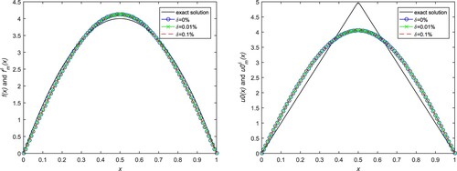
Example 5.3

We consider the source term and initial value are all piecewise functions $f\left(x\right)=\{\begin{array}{ll}x,& 0\le x<{\displaystyle \frac{1}{2}},\\ 1-x,& {\displaystyle \frac{1}{2}}\le x\le 1,\end{array}$ and $u^0\left(x\right)=-|x-\frac{1}{2}|+\frac{1}{2}.$ The exact and numerical solutions are given in Figures 4 and 5 in the case of $\alpha =0.3$, 0.9, respectively, and the exact solution can be obtained by the Fourier series expansion method. Similarly, the reconstructed solutions of $f\left(x\right)$ and $u^0\left(x\right)$ from the noisy data $g_1^{\delta }\left(x\right)$ and $g_2^{\delta }\left(x\right)$ are also performed, where the noisy level δ is taken as $0\mathrm{\%}$, $0.01\mathrm{\%}$ and $0.1\mathrm{\%}$, respectively. Some computation parameters α, ${ϵ}_f$ and ${ϵ}_{u^0}$ for exact input and noisy data respectively are given in Tables 2 and 3. From the two tables, we observe that the relative errors of $f\left(x\right)$ and $u^0\left(x\right)$ become larger as the increasement of the noisy level δ.

Figure 4. Numerical results for initial value and source term in Example 5.3. (a) Source term with $\alpha =0.3$ $T_1=0.2$, $T_2=0.5$. (b) Initial value with $\alpha =0.3$ $T_1=0.2$, $T_2=0.5$.

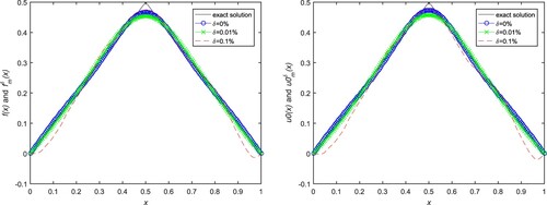
Figure 5. Numerical results for initial value and source term in Example 5.3. (a) Source term with $\alpha =0.9$ $T_1=0.2$, $T_2=0.5$. (b) Initial value with $\alpha =0.9$ $T_1=0.2$, $T_2=0.5$.

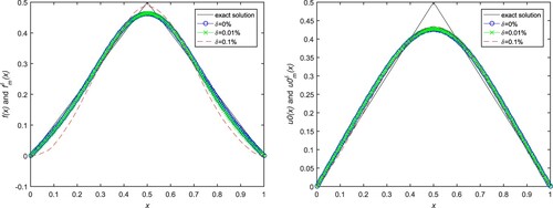
Table 2. The relative error and the stop steps of $f\left(x\right)$ in parentheses for Example 5.3 with different δ and α.

$\alpha ╲\delta$	$0\mathrm{\%}$	$0.01\mathrm{\%}$	$0.1\mathrm{\%}$
0.1	$0.0213\left(4\right)$	$0.0384\left(4\right)$	$0.0685\left(4\right)$
0.3	$0.0224\left(4\right)$	$0.0402\left(4\right)$	$0.0787\left(4\right)$
0.5	$0.0219\left(4\right)$	$0.0404\left(4\right)$	$0.0998\left(4\right)$

Table 3. The relative error and the stop steps of $u^0\left(x\right)$ in parentheses for Example 5.3 with different δ and α.

$\alpha ╲\delta$	$0\mathrm{\%}$	$0.01\mathrm{\%}$	$0.1\mathrm{\%}$
0.1	$0.0211\left(4\right)$	$0.0385\left(4\right)$	$0.0640\left(4\right)$
0.3	$0.0219\left(4\right)$	$0.0404\left(4\right)$	$0.0969\left(4\right)$
0.5	$0.0216\left(4\right)$	$0.0411\left(4\right)$	$0.1070\left(4\right)$

Example 5.4

Consider source term and initial value are the combination of piecewise functions and smooth functions $f\left(x\right)=\{\begin{array}{ll}1,& 0\le x<0.2,\\ 5,& 0.2\le x<0.4,\\ 1+\sin 8\pi x,& 0.4\le x<1,\end{array}$ and $u^0\left(x\right)=\{\begin{array}{ll}0,& 0\le x<0.2,\\ 2,& 0.2\le x<0.4,\\ \sin 8\pi x,& 0.4\le x\le 1.\end{array}$ Applying the Fourier transform method, we obtain the inexact solution of the example $\begin{array}{rl}u(x,t)& =\sum _{k=1}^{\mathrm{\infty }}\left[{\int }_0^{1}f\right(x)\sin (k\pi x)\mathrm{d}x\frac{1-E_{\alpha ,1}(-{\lambda }_k{t}^{\alpha })}{{\lambda }_k}\\ & +E_{\alpha ,1}(-{\lambda }_k{t}^{\alpha }){\int }_0^1{u}^0\left(x\right)\sin \left(k\pi x\right)\mathrm{d}x]\sin \left(k\pi x\right).\end{array}$ And the reconstructed solutions of $f\left(x\right)$ and $u^0\left(x\right)$ are obtained from the noisy datas $g_1^{\delta }\left(x\right)$ and $g_2^{\delta }\left(x\right)$. The exact solution and the numerical one are given in Figures 6 and  7. Some computation parameters α, ${ϵ}_f$ and ${ϵ}_{u^0}$ for exact input and noisy data are shown in Tables 4 and 5, respectively.

Figure 6. Numerical results for initial value and source term in Example 5.4. (a) Source term with $\alpha =0.3$ $T_1=0.04$, $T_2=0.3$. (b) Initial value with $\alpha =0.3$ $T_1=0.04$, $T_2=0.3$.

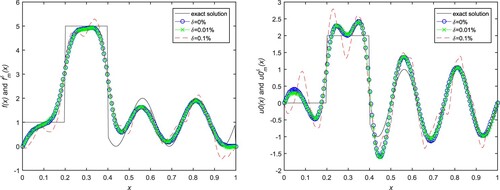
Figure 7. Numerical results for initial value and source term in Example 5.4. (a) Source term with $\alpha =0.9$ $T_1=0.04$ and $T_2=0.3$ (b) Initial value with $\alpha =0.9$ $T_1=0.04$ and $T_2=0.3$.

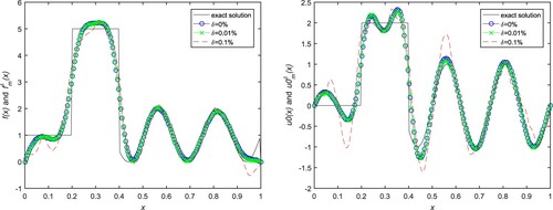
Table 4. The relative error and the stop steps of $f\left(x\right)$ in parentheses for Example 5.4 with different δ and α.

$\alpha ╲\delta$	$0\mathrm{\%}$	$0.01\mathrm{\%}$	$0.1\mathrm{\%}$
0.3	$0.2453\left(15\right)$	$0.2478\left(15\right)$	$0.2655\left(15\right)$
0.5	$0.2365\left(20\right)$	$0.2385\left(20\right)$	$0.2765\left(20\right)$

Table 5. The relative error and the stop steps of $u^0\left(x\right)$ in parentheses for Example 5.4 with different δ and α.

$\alpha ╲\delta$	$0\mathrm{\%}$	$0.01\mathrm{\%}$	$0.1\mathrm{\%}$
0.3	$0.2882\left(15\right)$	$0.2818\left(15\right)$	$0.4270\left(15\right)$
0.5	$0.2427\left(20\right)$	$0.2487\left(20\right)$	$0.4392\left(20\right)$

The comparisons between the exact solution and the approximate solution of the source term and the initial value for Examples 5.1–5.4 are shown in Figures 1–7 and various noisy levels are added into the data. From Figure 1, we can see the initial value and the source term change a little as the increasing of the noisy level, and the initial data becomes better than the source term. From Figures 2–7, because there are not exact solutions, the numerical fitness is not very satisfactory. All in all, the numerical results show that the reconstruction of the source term is more satisfactory than the initial value because of its regularity. And the smooth functions are more satisfactory than the piecewisely smooth functions under the different noisy levels.

In Tables 1–5, we show the relative numerical errors and the stop steps in parentheses for Examples 5.1, 5.3 and 5.4 with respective to different α and δ. It can be seen that the numerical error becomes larger while the noisy level becomes larger. The stop steps for Examples 5.1–5.3 are less than 5 and the one for Example 5.4 is less than 20, which means that the proposed method has a good convergence. In our opinion, the reconstruction of the non-smooth (or piecewisely smooth) functions is a little more difficult than the smooth functions.

6. Conclusion

In this paper, we devote to identifying the source term and the initial item in a time-fractional diffusion equation. The inverse problem is formulated as a minimization problem. The conjugate gradient algorithm with an appropriate stopping criterion is used to solve the regularized variational problem. And we construct a solution of the corresponding operator equation. In the end, four numerical examples are provided to show that the proposed method is effective and stable for solving the simultaneous inversion problem.

Disclosure statement

No potential conflict of interest was reported by the author(s).

Additional information

Funding

The work described in this article was supported by the National Natural Science Foundation of China (NNSF of China) [grant number 11326234], The Natural Science Foundation of Gansu Province (NSF of Gansu Province) [grant number 145RJZA099], Scientific research project of Higher School in Gansu Province [grant number 2014A-012], and Project of NWNU-LKQN [grant number NWNU-LKQN2020-08].

References

- Berkowitz B, Scher H, Silliman SE. Anomalous transport in laboratory-scale, heterogeneous porous media. Water Resour Res. 2000;36:149–158. DOI: 10.1029/1999WR900295.
- Metzler R, Klafter J. The random walk's guide to anomalous diffusion: a fractional dynamics approach. Phys Rep. 2000;339:77. DOI: 10.1016/S0370-1573(00)00070-3.
- Johansson BT, Lesnic D. A variational method for identifying a spacewise-dependent heat source. IMA J Appl Math. 2007;72:748-–760. DOI: 10.1093/imamat/hxm024.
- Johansson BT, Lesnic D. A procedure for determining a spacewise dependent heat source and the initial temperature. Appl Anal. 2008;87:265–276. DOI: 10.1080/00036810701858193.
- Metzler R, Klafter J. Subdiffusive transport close to thermal equilibrium: from the Langevin equation to fractional diffusion. Phys Rev E. 2000;61:6308. DOI: 10.1103/PhysRevE.61.6308.
- Raberto M, Scalas E, Mainardi F. Waiting-times and returns in high-frequency financial data: an empirical study. Phys A: Stat Mech Appl. 2002;314:749–755. Horizons in Complex Systems. DOI: 10.1016/S0378-4371(02)01048-8.
- Yuste SB, Acedo L, Lindenberg K. Reaction front in an A+B → C reaction-subdiffusion process. Phys Rev E. 2004;69:036126. DOI: 10.1103/PhysRevE.69.036126.
- Yuste S, Lindenberg K. Subdiffusion-limited reactions. Chem Phys. 2002;284:169–180. Strange Kinetics. DOI: 10.1016/S0301-0104(02)00546-3.
- Dhawan S, Machado JAT, Brzeziński DW, et al. A Chebyshev wavelet collocation method for some types of differential problems. Symmetry. 2021;13:4. Available from: https://www.mdpi.com/2073-8994/13/4/536.
- Kumar S, Chauhan R, Abdel-Aty AH, et al. A study on fractional tumour C immune C vitamins model for intervention of vitamins. Results in Physics. 2021;33:2211–3797. DOI: 10.1016/j.rinp.2021.104963.
- Kumar S, Kumar R, Osman MS, et al. A wavelet based numerical scheme for fractional order SEIR epidemic of measles by using Genocchi polynomials. Numer Meth Partial Differ Equ. 2021;37:1250–1268. DOI: 10.1002/num.22577.
- Nisar KS, Ciancio A, Ali KK, et al. On beta-time fractional biological population model with abundant solitary wave structures. Alexandria Eng J. 2022;61:1996–2008. DOI: 10.1016/j.aej.2021.06.106.
- Iqbal M.A, Wang Y, Miah MM, et al. Study on Date-Jimbo-Kashiwara-Miwa equation with conformable derivative dependent on time parameter to find the exact dynamic wave solutions. Fractal and Fractional. 2022;6:4. Available from: https://www.mdpi.com/2504-3110/6/1/4.
- Cuahutenango-Barro B, Taneco-Hern???ndez MA, Lv Y-P, et al. Analytical solutions of fractional wave equation with memory effect using the fractional derivative with exponential kernel. Results in Physics. 2021;25:104148. DOI: 10.1016/j.rinp.2021.104148.
- Hakimeh M, Sunil K, Shahram R, et al. A theoretical study of the Caputo-Fabrizio fractional modeling for hearing loss due to Mumps virus with optimal control. Chaos, Solitons, Fractals. 2021;144:0960–0779. DOI: 10.1016/j.chaos.2021.110668.
- Kumar D.S, Chauhan R, Momani S, et al. Numerical investigations on COVID-19 model through singular and non-singular fractional operators. Numer Meth Partail Differ Equ. 2020; DOI: 10.1002/num.22707.
- Hemen D, Sunil Dr K, Ajay K, et al. A study on fractional host-parasitoid population dynamical model to describe insect species. Numer Meth Partail Differ Equ. 2020;37:1673–1962. DOI: 10.1002/num.22603.
- Kumar A, Kumar S. A study on eco-epidemiological model with fractional operators. Chaos, Solitons, Fractals. 2022;156:0960–0779. DOI: 10.1016/j.chaos.2021.111697.
- Arqub O.A, Al-Smadi M, Almusawa H, et al. A novel analytical algorithm for generalized fifth-order time-fractional nonlinear evolution equations with conformable time derivative arising in shallow water waves. Alexandria Eng J. 2022;61:5753–5769. DOI: 10.1016/j.aej.2021.12.044.
- Chi G, Li G, Jia X. Numerical inversions of a source term in the FADE with a Dirichlet boundary condition using final observations. Comput Math Appl. 2011;62:1619–1626. DOI: 10.1016/j.camwa.2011.02.029.
- Jiang D, Li Z, Liu Y, et al. Weak unique continuation property and a related inverse source problem for time-fractional diffusion-advection equations. Inverse Probl. 2017;33:055013. DOI: 10.1088/1361-6420/aa58d1.
- Ruan Z, Yang Z, Lu X. An inverse source problem with sparsity constraint for the time-fractional diffusion equation. Adv Appl Math Mech. 2016;8:1-–18. DOI: 10.4208/aamm.2014.m722.
- Slodička M, Šišková K. An inverse source problem in a semilinear time-fractional diffusion equation. Comput Math Appl. 2016;72:1655–1669. DOI: 10.1016/j.camwa.2016.07.029.
- Wang W, Yamamoto M, Han B. Numerical method in reproducing kernel space for an inverse source problem for the fractional diffusion equation. Inverse Probl. 2013;29:095009. DOI: 10.1088/0266-5611/29/9/095009.
- Wei T, Li XL, Li YS. An inverse time-dependent source problem for a time-fractional diffusion equation. Inverse Probl. 2016;32:085003. DOI: 10.1016/j.amc.2018.05.016.
- Wei T, Wang J. A modified quasi-boundary value method for an inverse source problem of the time-fractional diffusion equation. Appl Numer Math. 2014;78:95–111. DOI: 10.1016/j.apnum.2013.12.002.
- Zhang Y, Xu X. Inverse source problem for a fractional diffusion equation. Inverse Probl. 2011;27:035010. DOI: 10.1088/0266-5611/27/3/035010.
- Hào DN, Duc NV, Lesnic D. Regularization of parabolic equations backward in time by a non-local boundary value problem method. IMA J Appl Math. 2010;75:291–315. DOI: 10.1093/imamat/hxp026.
- Oanh NTN. A splitting method for a backward parabolic equation with time-dependent coefficients. Comput Math Appl. 2013;65:17–28. DOI: 10.1016/j.camwa.2012.10.005.
- Šišková K, Slodička M. Recognition of a time-dependent source in a time-fractional wave equation. Appl Numer Math. 2017;121:1–17. DOI: 10.1016/j.apnum.2017.06.005.
- Yan XB, Wei T. Inverse space-dependent source problem for a time-fractional diffusion equation by an adjoint problem approach. J Inverse Ill-Posed Probl. 2019;27:1–16. DOI: 10.1515/jiip-2017-0091.
- Sakamoto K, Yamamoto M. Initial value/boundary value problems for fractional diffusion-wave equations and applications to some inverse problems. J Math Anal Appl. 2011;382:426–447. DOI: 10.1016/j.jmaa.2011.04.058.
- Li YS, Sun LL, Zhang ZQ, et al. Identification of the time-dependent source term in a multi-term time-fractional diffusion equation. Numer Algorithms. 2019;82:1279–1301. DOI: 10.1007/s11075-019-00654-5.
- Djennadi S, Shawagfeh N, Inc M, et al. The Tikhonov regularization method for the inverse source problem of time fractional heat equation in the view of ABC-fractional technique. Physica Scripta. 2021;96:094006. DOI: 10.1088/1402-4896/ac0867.
- Wang B, Yang B, Xu M. Simultaneous identification of initial field and spatial heat source for heat conduction process by optimizations. Adv Difference Equ.. 2019;2019:1–6. DOI: 10.1186/s13662-019-2344-5.
- Ruan Z, Yang JZ, Lu X. Tikhonov regularisation method for simultaneous inversion of the source term and initial data in a time-fractional diffusion equation. East Asian J Appl Math. 2015;5:273–300. DOI: 10.4208/eajam.310315.030715a.
- Wen J, Liu ZX, Yue CW, et al. Landweber iteration method for simultaneous inversion of the source term and initial data in a time-fractional diffusion equation. J Appl Math Comput. 2021; 1–32. DOI: 10.1007/s12190-021-01656-0.
- Daniel JW. The conjugate gradient method for linear and nonlinear operator equations. SIAM J Numer Anal. 1967;4:10–26. DOI: 10.1137/0704002.
- Daniel JW. The conjugate gradient method for linear and nonlinear operator equations [thesis (PhD)]. ProQuest LLC. Ann Arbor, MI: Stanford University; 1965.
- Podlubny I. Fractional differential equations. Academic Press, Inc.: San Diego, CA; 1999. (Mathematics in Science and Engineering; 198).
- Hanke M, Hansen PC. Regularization methods for large-scale problems. Surveys Math Indust. 1993;3:253–315.