Identification method of excitation forces based on Kalman filter

ABSTRACT

To identify the excitation forces of a vibration system, two identification methods are proposed, which take the displacement and acceleration responses of the system as input parameters. These two methods are based on the Kalman filter and minimum variance estimation method. The accumulation of identification errors in the iterative process is prevented through the non-iterative identification formula of the excitation force. The identification results and robustness of these two methods with different input parameters are analyzed. The results show that the identification accuracy of the method with acceleration as the input parameter is better than the method with displacement as the input parameter. Four types of hammer strike tests are performed. The test results show that the identification method with acceleration as the input parameter is effective in practical applications.

KEYWORDS:

• Excitation force
• identification method
• Kalman filter
• minimum variance estimation

MATHEMATICS SUBJECT CLASSIFICATION:

• TB21

1. Introduction

For a vibrating mechanical system, the calculation accuracy of the system excitation force is very important. It affects the system vibration response characteristics and the system fatigue life. Owing to the constraints of the tooling and sensor layout space, it is difficult to test the excitation force directly in practical engineering applications. Common excitation identification methods can be divided into direct, regularization, and Kalman filter methods.

The direct method [1–3] is a simple method used in practical engineering applications. In this method, a dynamic model of the vibration system needs to be established first. The precise values of each parameter of the system need to be obtained. The identification process is usually performed in the frequency domain. As a result, the amplitude and phase of the excitation force in the frequency domain can be identified.

The basic idea of the regularization method is to find a set of suitable regularization solutions by imposing reasonable additional conditions or boundary constraints on the ill-posed problem and then selecting the most suitable solution of the equation. Zhang et al. [4] identified the excitation force of the time-invariant system by the conjugate gradient method. Traditional regularization methods assume that the force has a zero-mean distribution, which is often inconsistent with reality. Some recent studies have combined Bayesian methods with regularization to solve this problem [5,6].

In view of the ill conditioned matrix problem in the inversion process and the influence of measurement noise on the identification of exciting force, a time-domain identification method based on Kalman filter method is proposed. Kalman filter method can estimate the optimal state of the system, which was first proposed by Dr. Kalman in 1961. Firstly, a Riccati type nonlinear differential equation of the optimal filtering error covariance matrix obtained by Kalman filter is derived. The solution of this ‘variance equation’ completely specifies the optimal filter for either finite or infinite smoothing intervals and stationary or nonstationary statistics [7]. However, the traditional Kalman filter method can only reduce the influence of noise, and the traditional method needs to be modified to identify the excitation force. Ma et al. [8] proposed an online force estimation method based on least square filter and recursive Kalman filter. The filter uses a set of linear state equations to simulate system dynamics. The practicability and accuracy of the estimation method are verified by numerical simulation. The input force of the free end concentrated mass cantilever beam is estimated by the output response. On this basis, an inverse estimation method of input force of nonlinear structural system is proposed. Input force estimation algorithms for two-dimensional or three-dimensional nonlinear structural systems are being developed [9]. Extended Kalman filter (EKF) needs to calculate Jacobian matrix. For the complicated calculation process of input and output Jacobian Kalman filter, a simplified multi state estimation method based on EKF is proposed. Louren et al. [10] proposed an enhanced Kalman filter for force identification in structural dynamics, in which the unknown force is included in the state vector and estimated in combination with the state. The noise is modelled as a random process. It is assumed that the noise exists not only in the measured value, but also in the state variable, which explains the modelling error to a certain extent. Reference [11] studies a model-based data fusion method (strain and acceleration), which greatly improves the accuracy of augmented Kalman filter (AKF) method in identifying exciting force. Yang et al. [12] proposed the iterative formula of excitation force. The estimated value of the exciting force at the current time is affected by the estimated value of the exciting force at the previous time. This method can easily lead to error accumulation. The above literature introduces some Kalman filter extension methods. The estimated exciting force of these methods participate in the iteration, which affect the accuracy of the final identification results.

At present, most excitation force identification methods use acceleration or displacement response as system input. Wu et al. [13] proposed a time-varying excitation force identification method based on structural system response measurement. Firstly, the acceleration response of the system is collected, and a simple Kalman filter is used to establish the regression model between the residual innovation and the input excitation force. Based on the regression model, a recursive least squares estimation method is proposed. Lin [14] proposed a new input estimation inverse method to determine the time-varying excitation force, which identifies the input excitation force by measuring the displacement response of the nonlinear system. The algorithm includes extended Kalman filter with recursive estimator. Naets et al. [15] used Kalman filter and regularization method to take the unknown force as the parameter of system state vector. Taking the acceleration response as the input, the extended Kalman filter method is used to calculate the extended state vector and identify the unknown excitation force. They used displacement or acceleration responses as input parameters, but did not compare the effects of the two inputs on the results.

The identification process of this study is divided into two steps: firstly, the improved Kalman filter method is used to obtain the optimal state estimation of the system, and the excitation force is calculated by using the optimal state estimation of the system obtained in the first step, so as to avoid the influence of process noise and observation noise on the identification results. Different from other Kalman estimation methods [8–12], the estimated value of excitation force does not participate in the next iterative calculation, which can prevent the accumulation of excitation force estimation error in the identification process. Based on this identification method, two identification methods are proposed. The input parameters are displacement and acceleration response. The above literature uses displacement or acceleration response as input parameters and does not compare the two input methods. This study compares the two methods.

The structure of this paper is as follows. Firstly, the calculation formulas of the two methods are derived. The accuracy and robustness of the two methods are compared. The effects of structural input parameters (stiffness and damping coefficient) and state input parameters (initial values of displacement and velocity) on the identification results are analyzed. Finally, the correctness and effectiveness of the identification method with acceleration as input are verified by hammering test. The identification results show that the identification method with acceleration as input is effective in practical application.

2 Derivation of excitation force identification formula based on Kalman filter method

2.1 Establishment of state space model of vibration system

The differential equation of the system vibrations can be written as follows: (1) $m\ddot{x}\left(t\right)+c\dot{x}\left(t\right)+Kx\left(t\right)=F\left(t\right)$(1) where m denotes the mass of the system, c and K represent the damping coefficient and stiffness of the mounting system, respectively, $x\left(t\right)$,$\dot{x}\left(t\right)$ and $\ddot{x}\left(t\right)$ are the displacement, velocity, and acceleration responses of the system at t time, respectively, and $F\left(t\right)$ is the excitation force of the system at t time.

2.1.1 State space model with displacement response value as observation

The continuous state space equation is used to describe the vibration process of the system. When the displacement response of the system is taken as the observed quantity, equation (1) can be written as follows: (2) $\begin{array}{rl}\dot{X}\left(t\right)& =AX\left(t\right)+BF\left(t\right)\end{array}$(2) (3) $\begin{array}{rl}Z\left(t\right)& =HX\left(t\right)\end{array}$(3) where $X\left(t\right)$ is the state vector of the system, $A$ is the state transition matrix, $B$ is the position matrix of the excitation force, $Z\left(t\right)$ is the response observation signal corresponding to the state of the system, and H is the observation matrix. These are defined as follows: $X\left(t\right)=\left[\begin{array}{c}x\left(t\right)\\ \dot{x}\left(t\right)\end{array}\right]$,$A=\left[\begin{array}{cc}0& 1\\ -K/m& -c/m\end{array}\right]$, $B=\left[\begin{array}{c}0\\ 1/m\end{array}\right]$, $H=\left[\begin{array}{cc}1& 0\\ 0& 0\end{array}\right]$.

For computation, the continuous state space equation is discretized as follows: (4) $\begin{array}{rl}X\left(k+1\right)& =CX\left(k\right)+DF\left(k\right)+w\left(k\right),\end{array}$(4) (5) $\begin{array}{rl}Z\left(k\right)& =HX\left(k\right)+v\left(k\right),\end{array}$(5) where $w\left(k\right)$ and $v\left(k\right)$ are the system and observation noise, respectively. Their variances are represented by $Q$ and $R,$respectively. $C$ is state transition matrix of the discrete system, and $D$ is position matrix of the excitation force of the discrete system: $C=\text{exp}\left(A\mathrm{\Delta }T\right)$ and $D=\underset{0}{\overset{\mathrm{\Delta }T}{\int }}\text{exp}\left(A\tau \right)Bd\tau$.

2.1.2 State space model with acceleration response value as observation

When the acceleration of the system is observed, equation (1)(1) $m\ddot{x}\left(t\right)+c\dot{x}\left(t\right)+Kx\left(t\right)=F\left(t\right)$(1) can be written as follows: (6) $Y\left(t\right)=H_{1}X\left(t\right)+H_{2}F\left(t\right)$(6) where $Y\left(t\right)$ is the state matrix of the system, $H_1$ is the state transition matrix, and $H_2$ is the position matrix of the excitation forces. These are defined as follows: $Y\left(t\right)=\left[\begin{array}{c}0\\ \ddot{x}\left(t\right)\end{array}\right]$, $H_1=\left[\begin{array}{cc}0& 0\\ -K/m& -c/m\end{array}\right]$, and $H_2=\left[\begin{array}{cc}0& 0\\ 0& 1/m\end{array}\right]$.

An observational equation is defined as follows: (7) $Z\left(t\right)=H_{3}Y\left(t\right)+v\left(t\right),$(7) where $Z\left(t\right)$ is the acceleration response observation signal corresponding to the system state, $v\left(t\right)$ is the observation noise, and $H_3$ is the observation matrix, defined as follows: $H_3=\left[\begin{array}{cc}0& 0\\ 0& 1\end{array}\right]$.

For computation, the continuous state space equations are discretized, and the following results are obtained: (8) $\begin{array}{rl}X\left(k\right)& =CX\left(k-1\right)+DF\left(k-1\right)+w\left(k-1\right),\end{array}$(8) (9) $\begin{array}{rl}Y\left(k\right)& =H_{1}X\left(k\right)+H_{2}F\left(k\right),\end{array}$(9) (10) $\begin{array}{rl}Z\left(k\right)& =H_{3}Y\left(k\right)+v\left(k\right),\end{array}$(10) where $w\left(k-1\right)$ is the process noise matrix of the system.

2.2 Optimal state estimation under unknown excitation force

2.2.1 Optimal state estimation based on displacement response value

The prediction equation for the state in the Kalman filter algorithm is as follows: (11) $\overline{X}\left(k|k-1\right)=C\hat{X}\left(k-1|k-1\right)+DF\left(k-1\right),$(11) where $F\left(k-1\right)$ is known. (12) ${\overline{X}}^{\ast }\left(k|k-1\right)=C\hat{X}(k-1|k-1)$(12)

The innovation functions $e_1\left(k\right)$ and $e_2\left(k\right)$ are defined by (13) $\begin{array}{rl}{e}_1\left(k\right)& =X\left(k\right)-{\overline{X}}^{\ast }\left(k|k-1\right),\end{array}$(13) (14) $\begin{array}{rl}{e}_2\left(k\right)& =X\left(k\right)-\hat{X}\left(k|k\right),\end{array}$(14) $e_1$ is a new error expression introduced in this method, which represents the state prediction error when the excitation force is not considered. It is different from the state prediction error in the Kalman filter. $e_2$represents the state estimation error.

The innovation function ${\tilde{y}}_k$ is defined by (15) ${\tilde{y}}_k=Z\left(k\right)-H{\overline{X}}^{\ast }\left(k|k-1\right).$(15)

The residual ${\tilde{y}}_k$ contains information about the excitation force, as well as the influence of process and observation noise. Owing to the influence of the process noise and the observation noise on ${\tilde{y}}_k$, the preliminary estimated value of the excitation force calculated by $K$ is not accurate, and there is an error between the estimated and real values of the excitation force. Therefore, through the residual ${\tilde{y}}_k$, the estimated value of the excitation force calculated by $K$ is only used to construct a complete filtering process and is not regarded as the final result of the excitation force identification.

Another expression of ${\tilde{y}}_k$ can be obtained from equations (4), (5), and (11): (16) ${\tilde{y}}_k=HDF\left(k-1\right)+e_3\left(k\right),$(16) where $e_3\left(k\right)=H\left(C{e}_2\left(k-1\right)+w_{k-1}\right)+v_k$ [14].

From equation (16), the following can be obtained: (17) $\begin{array}{rl}\hat{F}\left(k-1\right)& =D^{-1}{H}^{-1}{\tilde{y}}_k,\end{array}$(17) (18) $\begin{array}{rl}F\left(k-1\right)& =D^{-1}{H}^{-1}\left[{\tilde{y}}_k-e_3\left(k\right)\right].\end{array}$(18)

The innovation function $e_4\left(k\right)$ is defined as (19) $e_4\left(k\right)=F\left(k\right)-\hat{F}\left(k\right),$(19) where $e_4\left(k\right)$ is the error between the initial estimated and real values of the exciting force. In this method, $e_4\left(k\right)$ is regarded as a third kind of noise, separate from process and observation noise.

The following can be obtained from equations (17) and (18): (20) $e_4\left(k-1\right)=-D^{-1}{H}^{-1}{e}_3\left(k\right)=-D^{-1}\left[C{e}_2\left(k\right)+w_{k-1}+H^{-1}{v}_k\right].$(20)

After obtaining the estimate of the excitation force, it is added to state prediction equation (11) to correct the state prediction, yielding the following: (21) $\overline{X}\left(k|k-1\right)=C{\overline{X}}^{\ast }\left(k|k-1\right)+D\hat{F}\left(k-1\right).$(21)

The innovation function$e_5\left(k\right)$ is defined by (22) $e_5\left(k\right)=X\left(k\right)-\overline{X}\left(k|k-1\right),$(22) where $e_5\left(k\right)$ represents the state prediction error, which has the same meaning as the state prediction error in the Kalman filter method. The difference is that the state prediction error in the Kalman filter method is the calculation error caused by the process noise, while the state prediction error in the excitation force identification method proposed in this section is the calculation error caused by the system process noise and the initial estimation error of the excitation force. The covariance matrix is $P_5$, corresponding to the covariance matrix $P\left(k|k-1\right)$ of the state prediction error in the Kalman filter process.

The following is obtained from equations (4), (11), and (16): (23) $e_5\left(k\right)=C{e}_2\left(k\right)+D{e}_4\left(k-1\right)+w_k.$(23)

Thus, (24) $\begin{array}{rl}{P}_5& =E\left[\begin{array}{cc}{e}_5& e_5^{\text{T}}\end{array}\right]=E\left[\begin{array}{cc}\left(C{e}_2+D{e}_4+w\right)& {\left(C{e}_2+D{e}_4+w\right)}^{\text{T}}\end{array}\right]\\ & =-2C{P}_2{C}^{\text{T}}-H^{-1}R(H^{-1}{)}^{\text{T}}-Q\end{array}$(24) where $P_2$ corresponds to the state estimation error covariance matrix $P\left(k|k\right)$ in the Kalman filter process, and $Q$ is the covariance matrix of the system process.

The calculation formula for the gain $K\left(k\right)$ can be obtained by Kalman filter: (25) $K\left(k\right)=P\left(k|k-1\right)H^{\text{T}}[P\left(k|k-1\right)H^{\text{T}}+R{]}^{-1}$(25)

The state optimal estimate $\hat{X}\left(k|k\right)$ is as follows: (26) $\hat{X}\left(k|k\right)=\overline{X}\left(k|k-1\right)+K\left(k\right)\left[Z\left(k\right)-H\overline{X}\left(k|k-1\right)\right].$(26)

The state estimation error covariance matrix calculation formula is as follows: (27) $P\left(k|k\right)=\left[I-K\left(k\right)H\right]P\left(k|k-1\right),$(27) where $I$ is the unit matrix.

2.2.2 Optimal state estimation based on acceleration response value

It is assumed that the system state estimate $\hat{\mathrm{X}}(\text{k}-1|\text{k}-1)$ at time $k-1$ has been obtained, and the excitation force information is known. The state prediction equations are as follows: (28) $\begin{array}{rl}\overline{X}\left(k|k-1\right)& =C\hat{X}\left(k-1|k-1\right)+DF\left(k-1\right),\end{array}$(28) (29) $\begin{array}{rl}\overline{Y}\left(k|k-1\right)& =H_1\overline{X}\left(k|k-1\right)+H_{2}F\left(k\right).\end{array}$(29)

Since the excitation force is unknown, only an incomplete system state prediction can be obtained: (30) $\begin{array}{rl}{\overline{X}}^{\ast }\left(k|k-1\right)& =C\hat{X}\left(k-1|k-1\right),\end{array}$(30) (31) $\begin{array}{rl}{\overline{Y}}^{\ast }\left(k|k-1\right)& =H_1{\overline{X}}^{\ast }\left(k|k-1\right).\end{array}$(31)

The innovation functions $e_6\left(k\right)$ and $e_7\left(k\right)$ are obtained by (32) $\begin{array}{rl}{e}_6\left(k\right)& =Y\left(k\right)-{\overline{Y}}^{\ast }\left(k|k-1\right),\end{array}$(32) (33) $\begin{array}{rl}{e}_7\left(k\right)& =Y\left(k\right)-\hat{Y}\left(k|k\right),\end{array}$(33) where $e_7\left(k\right)$ represents the estimation error of the acceleration state of the system.

The innovation function ${\tilde{y}}_k$ is defined by (34) ${\tilde{y}}_k=Z\left(k\right)-{\overline{Y}}^{\ast }\left(k|k-1\right)=Z\left(k\right)-H_1{\overline{X}}^{\ast }\left(k|k-1\right).$(34)

From equations (4)–(7) and (23)–(26), another expression of ${\tilde{\mathrm{y}}}_{\text{k}}$ can be obtained: (35) ${\tilde{y}}_k=H_{2}F\left(k\right)+e_8\left(k\right),$(35) with $e_8\left(k\right)=H\left(C{e}_7\left(k-1\right)+w_{k-1}\right)+v_k$ [14].

Based on equation (30), the following equations are obtained: (36) $\begin{array}{rl}\hat{F}\left(k\right)& ={H_2}^{-1}{\tilde{y}}_k,\end{array}$(36) (37) $\begin{array}{rl}F\left(k\right)& ={H_2}^{-1}\left[{\tilde{y}}_k-e_8\left(k\right)\right].\end{array}$(37)

The innovation function $e_9\left(k\right)$ is defined as (38) $e_9\left(k\right)=F\left(k\right)-\hat{F}\left(k\right).$(38)

The following is obtained from equations (31) and (32): (39) $e_9\left(k\right)=-{H_2}^{-1}{e}_8\left(k\right)=-{H_2}^{-1}\left[H_{1}C{e}_7\left(k\right)+H_1{w}_{k-1}+v_k\right].$(39)

The excitation force estimate is added to the state prediction equation (24) to correct the state prediction, as follows: (40) $\overline{Y}\left(k|k-1\right)={\overline{Y}}^{\ast }\left(k|k-1\right)+H_2\hat{F}\left(k\right).$(40)

The innovation function $e_{10}\left(k\right)$ is defined by (41) $e_{10}\left(k\right)=Y\left(k\right)-\overline{Y}\left(k|k-1\right),$(41) where $e_{10}\left(k\right)$ represents the state prediction error, and the corresponding covariance matrix is $P_{10}$. The covariance matrix $P_{10}$ corresponds to the state prediction error covariance matrix $P(k|k-1)$ in the Kalman filter.

The following can be obtained from equations (6), (9), and (11): (42) $e_{10}\left(k\right)=C{e}_7\left(k-1\right)+D{e}_9\left(k\right)+w_{k-1}.$(42)

Thus, (43) $\begin{array}{rl}{P}_{10}& =E\left[\begin{array}{cc}{e}_{10}& e_{10}^T\end{array}\right]\\ & =\left(C-D{H}_2^{-1}{H}_1\right)P_7(C-D{H}_2^{-1}{H}_1{)}^T+\left(I-D{H}_2^{-1}{H}_1\right)Q(I-D{H}_2^{-1}{H}_1{)}^T\\ & +D{H}_2^{-1}R(H_2^{-1}{)}^T{D}^T.\end{array}$(43) where $P_7$ corresponds to the state estimation error covariance matrix $P\left(k|k\right)$ in the Kalman filter process.

The gain $K\left(k\right)$ calculation formula can be obtained by Kalman filter: (44) $K\left(k\right)=P\left(k|k-1\right)H_1^T[H_{1}P\left(k|k-1\right)H_1^{T}R{]}^{-1}$(44)

The state optimal estimate $\hat{Y}\left(k|k\right)$ is as follows: (45) $\hat{Y}\left(k|k\right)=\overline{Y}\left(k|k-1\right)+K\left(k\right)\left[Z\left(k\right)-H_3\overline{Y}\left(k|k-1\right)\right].$(45)

The state estimation error covariance matrix calculation formula is as follows: (46) $P\left(k|k\right)=\left[I-K\left(k\right)H_1\right]P\left(k|k-1\right).$(46)

2.3 Estimation method of unknown excitation force

The estimate of the excitation force can be directly calculated using equation (17) or (36). It is known from equation (15) or (34) that the innovation ${\tilde{y}}_k$ is the difference between the state measurement and the state prediction, which includes measurement noise. Therefore, the excitation forces estimated by equations (17) or (36) are affected by noise.

The optimal estimate of the state $\hat{X}\left(k|k\right)$ is the state prediction $\overline{X}(k|k-1)$. The measurement value $Z\left(k\right)$ takes the weighted average and is closest to the true state $X\left(k\right)$. The optimal estimate of the state $\hat{Y}\left(k|k\right)$ is the least-variance estimate obtained by taking the weighted average of the state prediction $\overline{Y}\left(k|k-1\right)$ and the measurement $Z\left(k\right)$, and it is the closest to the state $Y\left(k\right)$. Therefore, using the difference between the optimal estimate of the state and the state predictor to calculate the excitation force estimate can effectively avoid the interference of the measurement noise.

The innovation function ${\tilde{y}}_k^{\ast }$ when observing the system displacement response is defined as follows: (47) ${\tilde{y}}_k^{\ast }=\hat{X}\left(k|k\right)-{\overline{X}}^{\ast }(k|k-1)$(47)

The optimal estimated excitation force is then obtained: (48) ${\hat{F}}^{\ast }\left(k-1\right)=(D^{T}D{)}^{-1}{D}^T{\tilde{y}}_k^{\ast }$(48)

The innovation function${\tilde{y}}_k^{\ast }$ when the system acceleration response is the observation is as follows: (49) ${\tilde{y}}_k^{\ast }=\hat{Y}\left(k|k\right)-{\overline{Y}}^{\ast }(k|k-1)$(49)

The optimal estimated excitation force is then obtained using least squares: (50) ${\hat{F}}^{\ast }\left(k\right)=(H_2^T{H}_2{)}^{-1}{H}_2^T{\tilde{y}}_k^{\ast }$(50)

3 Calculation examples

3.1 Identification process and results

To verify the effectiveness of these two identification methods, a single degree-of-freedom system is used as the simulation object to establish its Simulink model. A sinusoidal excitation is considered as an example. The simulation models are constructed as shown in Figures 1 and 2.

Figure 1. Simulink model with displacement as input parameter.

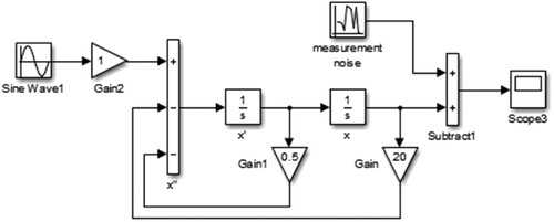
Figure 2. Simulink model with acceleration as input parameter.

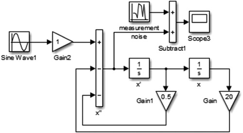
The dynamic response of the system displacement and acceleration are observed through the simulation. To simulate a real test situation, different levels of white noise are added to the observations.

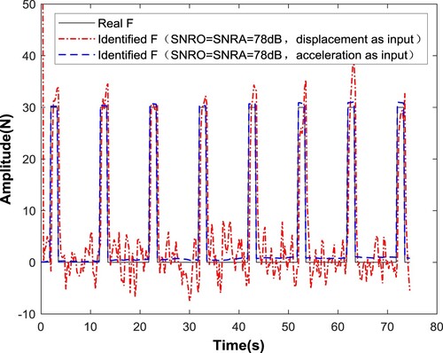
To study the identification accuracy of the method with displacement and acceleration as inputs, it was assumed that the signal-to-noise ratio (SNR) set in the algorithm was the same as that of the actual measurement noise, and both were 78 dB. The identification results are shown in Figure 3. SNRA denotes the SNR of the Gaussian white noise in the algorithm, and SNRO represents the SNR of Gaussian white noise observed in the experiment. The initial covariance matrices were all matrices with element 0. The relative errors of the maximum amplitude of the excitation identified by the displacement and acceleration were 12% and 3%, respectively. Therefore, under the same noise conditions, the identification method with acceleration as the input was better than that with displacement as the input.

Figure 3. Identification results of the excitation force with displacement and acceleration as inputs.

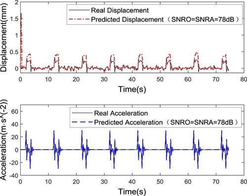
The state response prediction result is shown in Figure 4. From this figure, it can be seen that under the same SNR, the predicted value of acceleration is very close to the real value. The approximation between the predicted value of displacement and the true value is not as good as that of acceleration. It is confirmed that the recognition method with acceleration as input in Figure 3 has higher accuracy.

Figure 4. State prediction results with displacement and acceleration as inputs.

3.2 Influence of noise variance on identification result in algorithm

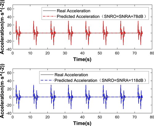
To study the influence of the SNR on the identification results, it is assumed that the SNR of observation noise is known, that is SNRO = SNRA. The SNRs are 78 and 81 dB, and the results of state prediction and excitation force identification are shown in Figures 5–8. When the displacement is used as the input, the average relative errors of the maximum amplitude are 7.97% and 6.18% for SNRs of 78 and 81 dB, respectively. When the acceleration is used as the input, the corresponding relative errors of the maximum amplitude are 1.99% and 0.11%, respectively. The results show that the higher the SNR is, the smaller the relative error of the identification result is. This is also reflected in the state prediction image.

Figure 5. Identification results of excitation force with displacement as inputs when SNRO = SNRA = 78 dB and SNRO = SNRA = 118 dB.

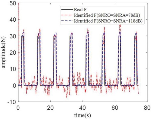
Figure 6. State prediction results with displacement as inputs when SNRO = SNRA = 78 dB and SNRO = SNRA = 118 dB.

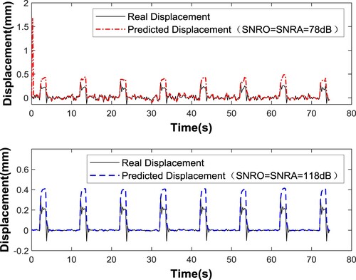
Figure 7. Identification results of the excitation force with acceleration as inputs when SNRO = SNRA = 78 dB and SNRO = SNRA = 118 dB.

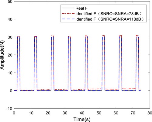
Figure 8. State prediction results with acceleration as inputs when SNRO = SNRA = 78 dB and SNRO = SNRA = 118 dB.

When the SNR of the measurement noise is not obtained or is difficult to obtain in a test, the initial value of the noise SNR is usually given by experience, and the SNRA in the algorithm is generally not equal to the actual SNRO. Taking the displacement as the input, a Gaussian white noise with an SNR of 78 dB is obtained, which is added to the system displacement response obtained by the Simulink simulation, but the noise SNRs in the algorithm are set to 38 and 118 dB. The identification results are shown in Figures 9 and 10. The average relative errors of the maximum excitation amplitude are 8.12% and 7.96% when SNRA = 38 and 118 dB, respectively. The results show that the set value of the SNR has no significant effect on the accuracy of the identification results; that is, the algorithm is not sensitive to the SNR in the initial value of the algorithm. The identification method with the acceleration as the input is also conducted using the same calculation process, and the identification results are shown in Figure 11. When SNRA = 38 and 118 dB, the average relative errors of the maximum amplitude are 2.01% and 1.99%, respectively. The same conclusion is that this method is not sensitive to the SNR in the initial value of the algorithm. The state prediction results when SNRA ≠ SNRO are shown in Figures 11 and 12. As can be seen from Figures 11 and 12, this method is insensitive to SNR. It has a better prediction effect with acceleration as input.

Figure 9. Identification results of the excitation force with displacement as the input when SNRA ≠ SNRO.

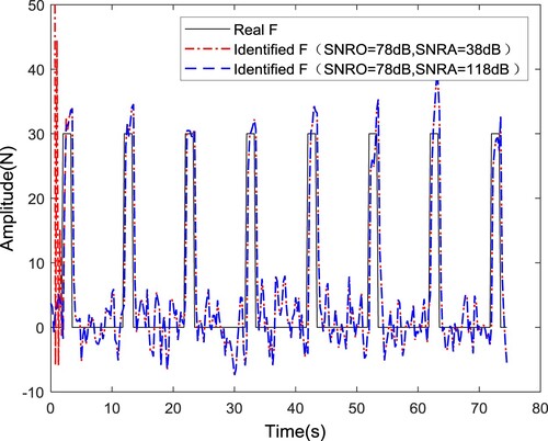
Figure 10. Identification results of excitation force with acceleration as the input when SNRA ≠ SNRO.

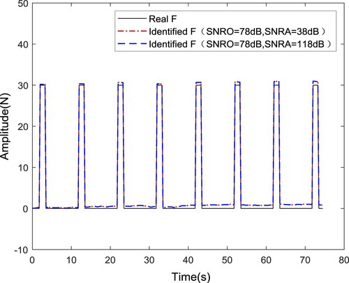
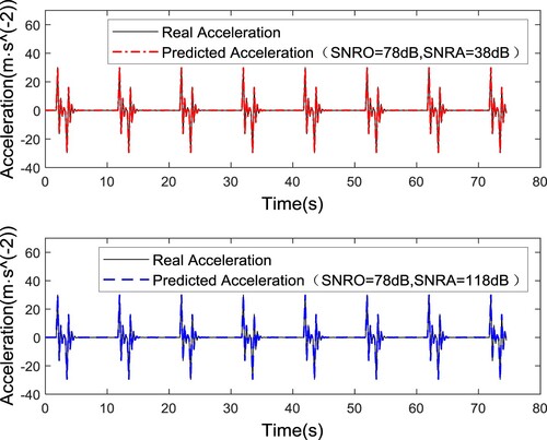
Figure 11. State prediction results with displacement as the inputs when SNRA ≠ SNRO

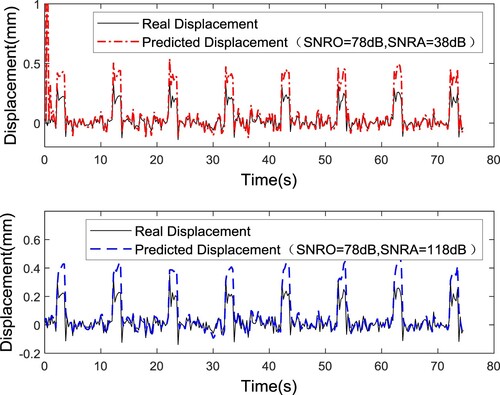
Figure 12. State prediction results with acceleration as the inputs when SNRA ≠ SNRO.

4 Robustness analysis

The input parameters of the identification method are the initial values of the displacement and velocity, the structural parameters of the system, the system response, the system noise variance, and the measurement noise variance. Since the initial value of the velocity and displacement and structural parameters such as the system stiffness and damping coefficient may be inaccurate, an error may occur when calculating the state prediction $\overline{X}\left(k|k-1\right)$ using equation (11).

The identification method with displacement as the input uses the displacement measurement and the state prediction to calculate the state estimate, and the state estimate is used in the subsequent iteration. The error of the initial parameter can be corrected after several iterations, and thereby, the system input parameter error is effectively eliminated. Therefore, the robustness of the method with displacement as the input is not analyzed.

For the method with acceleration as an input, the state prediction $\overline{X}\left(k|k-1\right)$ is only used to calculate the predicted acceleration at the next moment, and the acceleration observation value has no correction effect on the state prediction $\overline{X}\left(k|k-1\right)$, which affects the accuracy of the excitation force identification results. Therefore, it is necessary to perform robustness analysis.

In practical engineering applications, the relative error between the design and measured values of the structural parameters should be controlled to within 15%. It is known from the literature [13] that the relative error of the initial velocity obtained by the integration of the acceleration signal is less than 10%, and the relative error of the initial displacement is less than 15%. To analyze the influence of the structural parameters and the initial state parameters on the excitation force identification result, the SNR of the measurement noise is set to 118 dB. The deviations of the initial values of the structural parameters, such as the stiffness and damping coefficient, are ±20%, and the deviations of the initial velocity and initial displacement are ±20%. The values of each parameter are listed in Table 1. Based on these parameters, the excitation force is identified and calculated.

Table 1. Values of structural parameters and initial values of state.

	Actual value	−20%	+20%
Stiffness/N·m^−1	20	16	24
Damping coefficient/N·s·m^−1	0.5	0.4	0.6
Initial displacement/m	−0.05	−0.04	−0.06
Initial velocity/m·s^−1	0.2	0.16	0.24

An orthogonal experimental design is used to analyze the influence of the parameters on the accuracy of the identification results. The stiffness, damping coefficient, initial displacement, and initial velocity are defined as factors A, B, C, and D, respectively. The original, reduced, and increased parameter values in Table 1 are defined as levels 1, 2, and 3, respectively. A four-factor three-level orthogonal table is provided in Table 2.

Table 2. L₉ (3⁴) orthogonal table.

No.	A	B	C	D
1	20	0.5	−0.05	0.2
2	20	0.4	−0.06	0.16
3	20	0.6	−0.04	0.24
4	16	0.5	−0.06	0.24
5	16	0.4	−0.04	0.2
6	16	0.6	−0.05	0.16
7	24	0.6	−0.04	0.16
8	24	0.4	−0.05	0.24
9	24	0.6	−0.06	0.2

To facilitate the error comparison, five points at a maximum amplitude of the sinusoidal excitation are selected. The relative errors of the excitation force identification results at the five reference points of each experiment are calculated separately, and the results are shown in Table 3. When calculating the mean of the relative error, the absolute value of the negative relative error is presented. According to the mean values in Table 3, the relative error average values of the excitation force identification results of each factor at each level are calculated. For example, the average value of the relative error when the stiffness is at level 1 is the average of the relative errors of tests 1, 2, and 3. The calculation results are shown in Table 4. Based on the results in Table 4, the influences of each factor at each level on the identification results are plotted in Figure 13. The larger the slope of a curve is, the greater the influence of this parameter is on the identification results.

Table 3. Relative errors of excitation force identification results at five reference points in each experiment (%).

Number	Point 1	Point 2	Point 3	Point 4	Point 5	Average
1	−0.21	−0.95	1.14	−2.29	2.14	1.35
2	−3.75	4.93	−8.13	10.93	−13.13	8.18
3	3.40	−6.91	10.47	−15.55	17.44	10.75
4	−0.60	1.16	10.65	−9.24	11.18	6.56
5	1.22	1.60	6.89	−1.56	1.46	2.55
6	0.13	7.81	−1.97	8.37	−12.95	6.25
7	0.55	−2.26	−10.20	7.41	−10.54	6.19
8	−0.41	−10.91	6.41	−16.04	21.09	10.97
9	−2.21	−3.01	−4.97	−2.78	2.64	3.12

Table 4. Average relative errors of identification result at each level of each factor.

	Stiffness/N·m^−1	Damping coefficient/N·s·m^−1	Initial displacement/m	Initial velocity/m·s^−1
	A	B	C	D
Level 1	6.76	4.70	6.19	2.34
Level 2	5.11	7.23	6.50	6.87
Level3	6.76	6.71	5.95	9.43

Figure 13. Trend chart of each factor.

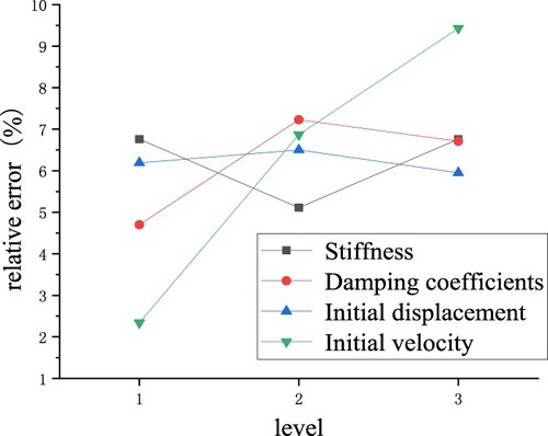
The orthogonal experiment results showed that the maximum relative error of the excitation force identification result is up to 21.09% when there are errors in the structural parameters, such as the stiffness and damping coefficients, and the initial values of the displacement and velocity. The trend graph shows that the initial velocity has a greater influence on the excitation force identification result than the initial displacement. The damping coefficient has a greater influence on the excitation force identification result than the stiffness.

5 Test verification

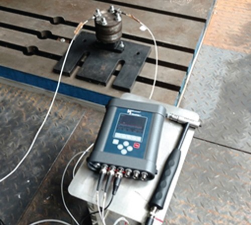
To verify the identification accuracy of the identification method, a single degree-of-freedom model is used for the test. The test model is composed of iron blocks, a rubber isolator, and a bottom plate. The iron blocks and the rubber isolator are fastened together by bolts, and the rubber isolator is regarded as a massless spring. Only vertical movement is considered.

The stiffness of the rubber isolator is 311 N/mm through the test. According to experience, the damping coefficient of the rubber isolator is assumed to be 0.05. The total mass of the iron blocks is 4.087 kg. The centre point of the upper surface of the block is hit by the hammer vertically, and the acceleration response of the vibration system in the vertical direction is recorded by the acceleration sensor, as shown in Figure 14.

Figure 14. Test equipment.

Four kinds of pulse excitation cases are selected: single pulse excitation, double impact excitation, two continuous pulse excitations in a short time (the first excitation amplitude is less than the second excitation amplitude), and two continuous pulse excitations in a short time (the first excitation amplitude is greater than the second excitation amplitude). The comparisons of the excitation force identification results are shown in Figures 15–18.

Figure 15. Single pulse excitation.

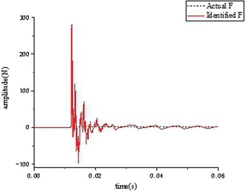
Figure 16. Double impact excitation.

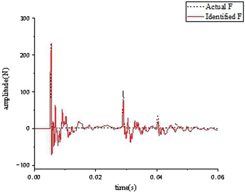
Figure 17. Two continuous pulse excitations (first excitation is smaller).

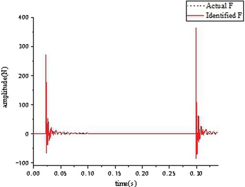
Figure 18. Two continuous pulse excitation (first excitation is larger).

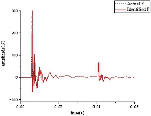
The algorithm identify the pulse excitations under the four kinds of pulse excitations accurately. In four cases, the maximum relative error of the amplitude peak of the excitation force is 17%. Because of the inertia of the blocks, the acceleration of the blocks does not converge to zero rapidly, so the identified force also does not converge to zero rapidly.

The identification and calculation process of the method with the displacement as the input is similar to the identification and calculation process of the method with the acceleration as the input. Thus, only the identification method with acceleration as the input is verified.

6 Conclusion

Based on an improved Kalman filter method and the least-variance estimate method, two identification methods with displacement and acceleration responses as inputs are presented. Under measurement noise, the identification results of these two methods are compared. The influence of the noise on the identification results in the algorithm is calculated and analyzed. Robustness analysis of the identification results is conducted. Finally, a single DOF model test is performed to verify the identification accuracy.

The main findings of this study are as follows:

1. Under the same measurement noise, the identification result accuracy with acceleration as the input is better than that with displacement as the input. Furthermore, the acceleration signal is much easier to measure. In the two identification methods, the smaller the measurement noise is, the smaller the relative error of the identification result become. These two methods are both insensitive to the initial value of the noise variance.

2. In the identification method with the acceleration as the input, the initial value of the velocity in the initial state has a greater influence on the identification result than the displacement, and the damping coefficient in the structural parameter has a greater influence on the identification result than the stiffness. However, the robustness of the method with displacement as an input is better.

3. The two excitation force identification methods proposed in the paper are also applicable to multi-DOFs systems.

Disclosure statement

No potential conflict of interest was reported by the author(s).

Data availability statement

All data included in this study are available upon request by contact with the corresponding author.

Additional information

Funding

This work were supported by the National Natural Science Foundation of China (No. 52175084, U20A20331) and Tianjin Key Laboratory of Aerospace Intelligent Equipment Technology Open Project Programme (No. ZNZB-2021-02).

References

- Tao JS, Liu GR, Lam KY. Excitation force identification of an engine with velocity data at mounting points. J Sound Vibr. 2001;242(2):321–331.
- Liu X-a, Yechi M, Chunlei J, et al. Identification and robustness analysis of powertrain excitation forces. Shock Vibr. 2020;2020:4536484.
- Chao M, Hongxing H, Feng X. The identification of external forces for a nonlinear vibration system in frequency domain. Proc Inst Mech Eng Part C J Mech Eng Sci. 2014;228(9):1531–1539.
- Zhang L, Yueyun C, Zichun Y, et al. Load identification using CG-TLS regularization algorithm. J Vibr Shock. 2014;33:159–164.
- Qiaofeng L, Lu Q. A revised time domain force identification method based on Bayesian formulation. Inter J Num Meth Eng. 2019;118(7):411–431.
- Gang Y, Sun H. A non-negative Bayesian learning method for impact force reconstruction. J Sound Vibr. 2019;457:354–367.
- Kalman RE, Bucy RS. New results in linear filtering and prediction theory. ASME J Basic Eng. 1961;83(1):95–108.
- Ma CK, Chang JM, Lin DC. Input forces estimation of beam structures by an inverse method. J Sound Vibr. 2003;259(2):387–407.
- Ma CK, Ho CC. An inverse method for the estimation of input forces acting on non-linear structural systems. J Sound Vibr. 2004;275(3-5):953–971.
- Lourens E, Reynders E, De Roeck G, et al. An augmented Kalman filter for force identification in structural dynamics. Mech Syst Signal Process. 2012;27:446–460.
- Babak K, Dyan M, Hongki J. Model-Based heterogeneous data fusion for reliable force estimation in dynamic structures under uncertainties. Sensors. 2017;17(11):2656.
- Yang JY, Pan SW, Lin S. Least-squares estimation with unknown excitations for damage identification of structures. J Eng Mech. 2007;133(1):12–21.
- Wu AL, Loh CH, Yang JN, et al. Input force identification:application to soil-pile interaction. Struct Contr Health Monit. 2010;16(2):223–240.
- Dong-Cherng L. Input estimation for nonlinear systems. Inverse Probl Sci Eng. 2010;18(5):673–689.
- Naets F, Cuadrado J, Desmet W. Stable force identification in structural dynamics using Kalman filtering and dummy-measurements. Mech Syst Signal Process. 2014;42:1–14.