A fast iterative method for identifying the radiogenic source for the helium production-diffusion equation

ABSTRACT

In this paper, we consider an inverse source problem for the helium production-diffusion equation. That is to determine a space-dependent source term in the helium production-diffusion equation from a noisy final data. Since the problem is ill-posed, we propose an effective iterative scheme to deal with the problem. More specifically, we use an acceleration technique to speed up a simple iterative scheme. We also give two kinds of convergence rates by using an a priori and a posteriori regularization parameter choice rule, respectively. Numerical examples are presented to illustrate the validity and effectiveness of the proposed method.

KEYWORDS:

• Inverse source problem
• ill-posed problem
• iterative regularization method
• convergence rate
• production-diffusion equation

2010 MATHEMATICS SUBJECT CLASSIFICATIONS:

• 11C08
• 11C99
• 11S05

1. Introduction

Inverse source problems play an important role in many branches of engineering applications, such as migration of groundwater, identification and control of pollution source and environmental protection. Due to its application background, in recent years, the inverse source problem has received much attention. Studies on the existence, uniqueness and stability can be found in [1–3]. Numerical methods may be found in [4–9] and related references therein.

In this paper, we consider an inverse radiogenic source problem for the helium production-diffusion equation (1) $\{\begin{array}{cl}{\displaystyle \frac{\mathrm{\partial }u(\rho ,t)}{\mathrm{\partial }t}}=\sigma \left(t\right)[{\displaystyle \frac{{\mathrm{\partial }}^{2}u(\rho ,t)}{\mathrm{\partial }{\rho }^2}}+{\displaystyle \frac{2}{\rho }}{\displaystyle \frac{\mathrm{\partial }u(\rho ,t)}{\mathrm{\partial }\rho }}]+f\left(\rho \right),& 0<t<T,0<\rho <R,\\ \underset{\rho \to 0}{lim}u(\rho ,t)\text{bounded},u(R,t)=0,& 0<t<T,\\ u(\rho ,0)=0,& 0<\rho <R.\end{array}$(1) where $0<{\sigma }_{-}\le \sigma \left(t\right)\le {\sigma }_{+}$(${\sigma }_{-}$ and ${\sigma }_{+}$ are constants) is the time-dependent diffusion coefficient. $f\left(\rho \right)$ corresponds to the spatial variable-dependent radiogenic source production. The object of this inverse radiogenic source problem is to reconstruct the source term $f\left(\rho \right)$ by using the given data (2) $u(\rho ,T)=\varphi \left(\rho \right),0<\rho <R,$(2) which is the final observation of the helium concentration. Since there may be some measurement errors in the data function $\varphi \left(\rho \right)$, the source function $f\left(\rho \right)$ has to be reconstructed from noisy data ${\varphi }^{\delta }\left(\rho \right)$. This model is closely connected to the (U-Th)/He isotopes dating, which is one method of low-temperature thermochronometry. For a detailed physical background, we refer to the paper[10–13]. Our model concerns the local helium concentration gradients resulting from the ejection of high-energy alpha particles from grain surfaces. It is assumed that the grain is of a spherical diffusion geometry, which is consistent with laboratory measurements of helium diffusion from apatite [13].

The inverse radiogenic source problem is ill-posed [11]. Therefore, in order to obtain a stable solution, some proper regularization methods are necessary. In [11], two regularization methods, the Tikhonov regularization and the spectral cutoff regularization are considered to obtain the regularized solution, where the regularization parameters are selected by a priori parameter choice rule. Several numerical examples show the efficiency and accuracy of the proposed methods. One criticism for the a priori parameter choice rules is that the regularization parameter depends on the priori information about the exact solution which is unavailable in practical problems, hence the parameter can not be explicitly computed. Therefore, researchers are more interested in the a posterior parameter choice rule. In [14], Zhang et al. formulate the spectral cutoff regularization method with the discrepancy principle in a uniform framework and adapt to solve the inverse radiogenic source problem. We note that both the Tikhonov and spectral cutoff regularized approximation solution in [11,14] are deduced in terms of the eigenfunction expansion, which may be not easy to calculate accurately if the diffusion coefficient is time dependent. Hence both the methods are not suitable for dealing with the inverse source problem (1(1) $\{\begin{array}{cl}{\displaystyle \frac{\mathrm{\partial }u(\rho ,t)}{\mathrm{\partial }t}}=\sigma \left(t\right)[{\displaystyle \frac{{\mathrm{\partial }}^{2}u(\rho ,t)}{\mathrm{\partial }{\rho }^2}}+{\displaystyle \frac{2}{\rho }}{\displaystyle \frac{\mathrm{\partial }u(\rho ,t)}{\mathrm{\partial }\rho }}]+f\left(\rho \right),& 0<t<T,0<\rho <R,\\ \underset{\rho \to 0}{lim}u(\rho ,t)\text{bounded},u(R,t)=0,& 0<t<T,\\ u(\rho ,0)=0,& 0<\rho <R.\end{array}$(1) ) – (2(2) $u(\rho ,T)=\varphi \left(\rho \right),0<\rho <R,$(2) ) with the diffusion coefficient depending on time variable.

Recently, a simple iterative scheme [15] was used to solve the inverse source problem (1(1) $\{\begin{array}{cl}{\displaystyle \frac{\mathrm{\partial }u(\rho ,t)}{\mathrm{\partial }t}}=\sigma \left(t\right)[{\displaystyle \frac{{\mathrm{\partial }}^{2}u(\rho ,t)}{\mathrm{\partial }{\rho }^2}}+{\displaystyle \frac{2}{\rho }}{\displaystyle \frac{\mathrm{\partial }u(\rho ,t)}{\mathrm{\partial }\rho }}]+f\left(\rho \right),& 0<t<T,0<\rho <R,\\ \underset{\rho \to 0}{lim}u(\rho ,t)\text{bounded},u(R,t)=0,& 0<t<T,\\ u(\rho ,0)=0,& 0<\rho <R.\end{array}$(1) )–(2(2) $u(\rho ,T)=\varphi \left(\rho \right),0<\rho <R,$(2) ), (3) $\begin{array}{rl}{f}^0& =0,\\ f^{k+1}& =f^k-\text{β}(K{f}^k-\varphi ),k=0,1,\dots ,\end{array}$(3) where the operator K is defined by $Kf=u(\cdot ,T)$ according to Equation (1(1) $\{\begin{array}{cl}{\displaystyle \frac{\mathrm{\partial }u(\rho ,t)}{\mathrm{\partial }t}}=\sigma \left(t\right)[{\displaystyle \frac{{\mathrm{\partial }}^{2}u(\rho ,t)}{\mathrm{\partial }{\rho }^2}}+{\displaystyle \frac{2}{\rho }}{\displaystyle \frac{\mathrm{\partial }u(\rho ,t)}{\mathrm{\partial }\rho }}]+f\left(\rho \right),& 0<t<T,0<\rho <R,\\ \underset{\rho \to 0}{lim}u(\rho ,t)\text{bounded},u(R,t)=0,& 0<t<T,\\ u(\rho ,0)=0,& 0<\rho <R.\end{array}$(1) ), β is a relaxation factor satisfying $0<\text{β}\Vert K\Vert <1$. This iterative process can be easily implemented, in each step, one only needs to solve a forward problem. It should be pointed out that the iterative scheme has been used to deal with sideways parabolic equation [16], backward diffusion problem [17] and inverse source problem [18] of time-fractional diffusion equation. As reported in [17,18], the iterative scheme (3(3) $\begin{array}{rl}{f}^0& =0,\\ f^{k+1}& =f^k-\text{β}(K{f}^k-\varphi ),k=0,1,\dots ,\end{array}$(3) ) is a very slow method, i.e. it needs far too many iteration steps to achieve the desired accuracy. Motivated by [19,20], in this paper, we construct the following iterative scheme, (4) $\begin{array}{rl}& z^k=f^k+{\alpha }_k(f^k-f^{k-1}),\\ & f^{k+1}=z^k-\text{β}(K{z}^k-\varphi ),k=0,1,\dots \end{array}$(4) with two initial elements $f^{-1}=f^0=0$. The sequence ${\alpha }_k$ is chosen as (5) ${\alpha }_k=\frac{k-1}{k+\eta },\eta \ge -1.$(5) Compared with the iterative scheme (3(3) $\begin{array}{rl}{f}^0& =0,\\ f^{k+1}& =f^k-\text{β}(K{f}^k-\varphi ),k=0,1,\dots ,\end{array}$(3) ), the iterative scheme (4(4) $\begin{array}{rl}& z^k=f^k+{\alpha }_k(f^k-f^{k-1}),\\ & f^{k+1}=z^k-\text{β}(K{z}^k-\varphi ),k=0,1,\dots \end{array}$(4) ) does not increase computation cost in each step except for one addition, which can be seen as an accelerated version of the iterative scheme (3(3) $\begin{array}{rl}{f}^0& =0,\\ f^{k+1}& =f^k-\text{β}(K{f}^k-\varphi ),k=0,1,\dots ,\end{array}$(3) ). We will show that the iterative scheme (4(4) $\begin{array}{rl}& z^k=f^k+{\alpha }_k(f^k-f^{k-1}),\\ & f^{k+1}=z^k-\text{β}(K{z}^k-\varphi ),k=0,1,\dots \end{array}$(4) ) is a regularization method under appropriate stopping rules. Our theoretical analysis shows that, compared with the iterative scheme (3(3) $\begin{array}{rl}{f}^0& =0,\\ f^{k+1}& =f^k-\text{β}(K{f}^k-\varphi ),k=0,1,\dots ,\end{array}$(3) ), the iterative scheme (4(4) $\begin{array}{rl}& z^k=f^k+{\alpha }_k(f^k-f^{k-1}),\\ & f^{k+1}=z^k-\text{β}(K{z}^k-\varphi ),k=0,1,\dots \end{array}$(4) ) can achieve the same convergence rate under both the a priori and a posteriori regularization parameter choice rules provided the parameter η in (5(5) ${\alpha }_k=\frac{k-1}{k+\eta },\eta \ge -1.$(5) ) is chosen large enough, but the number of iteration steps is much less than that of the iterative scheme (3(3) $\begin{array}{rl}{f}^0& =0,\\ f^{k+1}& =f^k-\text{β}(K{f}^k-\varphi ),k=0,1,\dots ,\end{array}$(3) ). Therefore, it is a more efficient method for solving the inverse source problem (1(1) $\{\begin{array}{cl}{\displaystyle \frac{\mathrm{\partial }u(\rho ,t)}{\mathrm{\partial }t}}=\sigma \left(t\right)[{\displaystyle \frac{{\mathrm{\partial }}^{2}u(\rho ,t)}{\mathrm{\partial }{\rho }^2}}+{\displaystyle \frac{2}{\rho }}{\displaystyle \frac{\mathrm{\partial }u(\rho ,t)}{\mathrm{\partial }\rho }}]+f\left(\rho \right),& 0<t<T,0<\rho <R,\\ \underset{\rho \to 0}{lim}u(\rho ,t)\text{bounded},u(R,t)=0,& 0<t<T,\\ u(\rho ,0)=0,& 0<\rho <R.\end{array}$(1) )–(2(2) $u(\rho ,T)=\varphi \left(\rho \right),0<\rho <R,$(2) ).

The rest of the paper is organized as follows. In Section 2, the iterative regularization method is proposed to obtain stable solution for the inverse source problem. Under a smoothness source condition on the exact source term, convergence rate estimates between the regularized solution and the exact solution are provided under both the a priori and a posteriori regularization parameter choice rules. In Section 3, three numerical examples are presented to illustrate the performance of the proposed method. Section 4 ends this paper with a conclusion and final remarks.

2. The iterative method and the related convergence rates

In this section, we will analyse the iterative regularization method and derive convergence rate estimates under a priori and a posteriori parameter choice rules. Throughout this paper, we denote by $L^2\left(\right[0,R];\rho )$ the Hilbert space of Lebesgue measurable function $u\left(\rho \right)$ with weight ρ on $[0,R]$. Denote by $〈\cdot ,\cdot {〉}_{\rho }$ and $\Vert \cdot {\Vert }_{\rho }$ the inner product and norm on $L^2\left(\right[0,R];\rho )$, respectively, given by $〈u,v{〉}_{\rho }={\int }_0^R\rho u\left(\rho \right)v\left(\rho \right)\mathrm{d}\rho \text{and}\Vert u{\Vert }_{\rho }={\left[{\int }_0^R\rho |u\right(\rho \left){|}^2\mathrm{d}\rho \right]}^{\frac{1}{2}}.$ In order to derive error estimates and convergence rate results for the iterative method (4(4) $\begin{array}{rl}& z^k=f^k+{\alpha }_k(f^k-f^{k-1}),\\ & f^{k+1}=z^k-\text{β}(K{z}^k-\varphi ),k=0,1,\dots \end{array}$(4) ), we introduce a substitution $u(\rho ,t)={\rho }^{-\frac{1}{2}}v(\rho ,t)$, then $v(\rho ,t)$ satisfies (6) $\{\begin{array}{cl}{\displaystyle \frac{\mathrm{\partial }v(\rho ,t)}{\mathrm{\partial }t}}=\sigma \left(t\right)[{\displaystyle \frac{{\mathrm{\partial }}^{2}v(\rho ,t)}{\mathrm{\partial }{\rho }^2}}+{\displaystyle \frac{1}{\rho }}{\displaystyle \frac{\mathrm{\partial }v(\rho ,t)}{\mathrm{\partial }\rho }}-{\displaystyle \frac{1}{4{\rho }^2}}v(\rho ,t\left)\right]+{\rho }^{\frac{1}{2}}f\left(\rho \right),& \begin{array}{l}0<t<T,\\ 0<\rho <R,\end{array}\\ \underset{\rho \to 0}{lim}{\rho }^{-\frac{1}{2}}v(\rho ,t)\text{bounded},v(R,t)=0,& 0<t<T,\\ v(\rho ,0)=0,& 0<\rho <R.\end{array}$(6) and the final observation of the helium concentration becomes (7) $v(\rho ,T)={\rho }^{\frac{1}{2}}\varphi \left(\rho \right),0<\rho <R.$(7) From the above discussion, we can reformulate the original inverse source problem (1(1) $\{\begin{array}{cl}{\displaystyle \frac{\mathrm{\partial }u(\rho ,t)}{\mathrm{\partial }t}}=\sigma \left(t\right)[{\displaystyle \frac{{\mathrm{\partial }}^{2}u(\rho ,t)}{\mathrm{\partial }{\rho }^2}}+{\displaystyle \frac{2}{\rho }}{\displaystyle \frac{\mathrm{\partial }u(\rho ,t)}{\mathrm{\partial }\rho }}]+f\left(\rho \right),& 0<t<T,0<\rho <R,\\ \underset{\rho \to 0}{lim}u(\rho ,t)\text{bounded},u(R,t)=0,& 0<t<T,\\ u(\rho ,0)=0,& 0<\rho <R.\end{array}$(1) )-(2(2) $u(\rho ,T)=\varphi \left(\rho \right),0<\rho <R,$(2) ): to reconstruct the source $f_{\rho }\left(\rho \right)$ from the given data ${\varphi }_{\rho }\left(\rho \right)$, where $f_{\rho }\left(\rho \right)={\rho }^{\frac{1}{2}}f\left(\rho \right),{\varphi }_{\rho }\left(\rho \right)={\rho }^{\frac{1}{2}}\varphi \left(\rho \right)$. If we define an operator $A:L^2[0,R;\rho ]\to L^2[0,R;\rho ]$ according to the system (6(6) $\{\begin{array}{cl}{\displaystyle \frac{\mathrm{\partial }v(\rho ,t)}{\mathrm{\partial }t}}=\sigma \left(t\right)[{\displaystyle \frac{{\mathrm{\partial }}^{2}v(\rho ,t)}{\mathrm{\partial }{\rho }^2}}+{\displaystyle \frac{1}{\rho }}{\displaystyle \frac{\mathrm{\partial }v(\rho ,t)}{\mathrm{\partial }\rho }}-{\displaystyle \frac{1}{4{\rho }^2}}v(\rho ,t\left)\right]+{\rho }^{\frac{1}{2}}f\left(\rho \right),& \begin{array}{l}0<t<T,\\ 0<\rho <R,\end{array}\\ \underset{\rho \to 0}{lim}{\rho }^{-\frac{1}{2}}v(\rho ,t)\text{bounded},v(R,t)=0,& 0<t<T,\\ v(\rho ,0)=0,& 0<\rho <R.\end{array}$(6) ), then the inverse source problem (6(6) $\{\begin{array}{cl}{\displaystyle \frac{\mathrm{\partial }v(\rho ,t)}{\mathrm{\partial }t}}=\sigma \left(t\right)[{\displaystyle \frac{{\mathrm{\partial }}^{2}v(\rho ,t)}{\mathrm{\partial }{\rho }^2}}+{\displaystyle \frac{1}{\rho }}{\displaystyle \frac{\mathrm{\partial }v(\rho ,t)}{\mathrm{\partial }\rho }}-{\displaystyle \frac{1}{4{\rho }^2}}v(\rho ,t\left)\right]+{\rho }^{\frac{1}{2}}f\left(\rho \right),& \begin{array}{l}0<t<T,\\ 0<\rho <R,\end{array}\\ \underset{\rho \to 0}{lim}{\rho }^{-\frac{1}{2}}v(\rho ,t)\text{bounded},v(R,t)=0,& 0<t<T,\\ v(\rho ,0)=0,& 0<\rho <R.\end{array}$(6) )–(7(7) $v(\rho ,T)={\rho }^{\frac{1}{2}}\varphi \left(\rho \right),0<\rho <R.$(7) ) can be formulated as the following operator equation: (8) $A{f}_{\rho }\left(\rho \right)={\varphi }_{\rho }\left(\rho \right),0<\rho <R.$(8) Applying the method of separation of variable for (6(6) $\{\begin{array}{cl}{\displaystyle \frac{\mathrm{\partial }v(\rho ,t)}{\mathrm{\partial }t}}=\sigma \left(t\right)[{\displaystyle \frac{{\mathrm{\partial }}^{2}v(\rho ,t)}{\mathrm{\partial }{\rho }^2}}+{\displaystyle \frac{1}{\rho }}{\displaystyle \frac{\mathrm{\partial }v(\rho ,t)}{\mathrm{\partial }\rho }}-{\displaystyle \frac{1}{4{\rho }^2}}v(\rho ,t\left)\right]+{\rho }^{\frac{1}{2}}f\left(\rho \right),& \begin{array}{l}0<t<T,\\ 0<\rho <R,\end{array}\\ \underset{\rho \to 0}{lim}{\rho }^{-\frac{1}{2}}v(\rho ,t)\text{bounded},v(R,t)=0,& 0<t<T,\\ v(\rho ,0)=0,& 0<\rho <R.\end{array}$(6) ) (see [11] for details), there holds ${\varphi }_{\rho }\left(\rho \right)=\sum _{n=1}^{\mathrm{\infty }}{\kappa }_n〈f_{\rho }\left(\rho \right),{\omega }_n\left(\rho \right){〉}_{\rho }{\omega }_n\left(\rho \right)$ with (9) ${\kappa }_n={\int }_0^T\exp [-{\lambda }_n{\int }_{\tau }^T\sigma (s\left)\mathrm{d}s\right]\mathrm{d}\tau ,{\lambda }_n=\left(\frac{n\pi }{R}\right),n=1,2,\dots ,$(9) and ${\omega }_n\left(\rho \right)=\frac{\sqrt{2}}{R{J}_{\frac{3}{2}}\left(n\pi \right)}{J}_{\frac{1}{2}}\left(\frac{n\pi \rho }{R}\right),n=1,2,\dots ,$ where $J_{\frac{1}{2}}\left(x\right)=(\frac{2}{\pi x}{)}^{\frac{1}{2}}\sin x$ and $J_{\frac{3}{2}}\left(x\right)=\left(\frac{2}{\pi x}{)}^{\frac{1}{2}}\right(\frac{\sin x}{x}-\cos x)$ are Bessel functions of fraction orders [21].

Consequently, A is a linear self-adjoint compact operator with eigenvalues ${\kappa }_n$ and eigenfunctions ${\omega }_n\left(\rho \right)$. It is easy to check that the eigenfunctions ${\omega }_1\left(\rho \right),{\omega }_2\left(\rho \right),\dots ,{\omega }_n\left(\rho \right),\dots$ form an orthonormal basis in $L^2\left(\right[0,R],\rho )$. Due to the fact that the eigenvalues ${\kappa }_n$ tends to zero, the inverse problem is ill-posed [22].

Based on the operator Equation (8(8) $A{f}_{\rho }\left(\rho \right)={\varphi }_{\rho }\left(\rho \right),0<\rho <R.$(8) ), we introduce the following iterative method, (10) $\begin{array}{rl}{z}_{\rho }^k& =f_{\rho }^k+{\alpha }_k(f_{\rho }^k-f_{\rho }^{k-1}),\\ f_{\rho }^{k+1}& =z_{\rho }^k-\text{β}(A{z}_{\rho }^k-{\varphi }_{\rho }),k=0,1,\dots \end{array}$(10) with initial elements $f_{\rho }^{-1}=f_{\rho }^0=0$, where β is a relaxation factor satisfying $0<\text{β}\Vert A\Vert \le 1$. According to the iterative scheme (10(10) $\begin{array}{rl}{z}_{\rho }^k& =f_{\rho }^k+{\alpha }_k(f_{\rho }^k-f_{\rho }^{k-1}),\\ f_{\rho }^{k+1}& =z_{\rho }^k-\text{β}(A{z}_{\rho }^k-{\varphi }_{\rho }),k=0,1,\dots \end{array}$(10) ), we have $f_{\rho }^k=(1+{\alpha }_{k-1})(I-\text{β}A)f_{\rho }^{k-1}-{\alpha }_{k-1}(I-\text{β}A)f_{\rho }^{k-2}+\text{β}{\varphi }_{\rho },$ where I is the identity operator. By induction, we can conclude that $f_{\rho }^k$ belongs to the Krylov subspace ${\mathcal{K}}_k(\text{β}A,\text{β}{\varphi }_{\rho })=\text{span}\{\text{β}{\varphi }_{\rho },(\text{β}A)\text{β}{\varphi }_{\rho },\dots ,(\text{β}A{)}^{k-1}\text{β}{\varphi }_{\rho }\}.$ Hence for the noisy data ${\varphi }_{\rho }^{\delta }\in L^2\left(\right[0,R],\rho )$ satisfying (11) $\Vert {\varphi }_{\rho }^{\delta }-{\varphi }_{\rho }{\Vert }_{\rho }\le \delta ,$(11) by using the eigenfunction expansion, the regularized solution can be given by (12) $f_{\rho }^{k,\delta }=R_k\left(\text{β}{\varphi }_{\rho }^{\delta }\right):=\sum _{n=1}^{\mathrm{\infty }}\text{β}{g}_k\left(\text{β}{\kappa }_n\right)〈{\varphi }_{\rho }^{\delta },{\omega }_n{〉}_{\rho }{\omega }_n,$(12) where $g_k$ is a polynomial of degree k−1. The residual satisfy (13) ${\varphi }_{\rho }^{\delta }-A{f}_{\rho }^k=\sum _{n=1}^{\mathrm{\infty }}(1-\text{β}{\kappa }_n{g}_k(\text{β}{\kappa }_n\left)\right)〈{\varphi }_{\rho }^{\delta },{\omega }_n{〉}_{\rho }{\omega }_n.$(13) If we define $r_k\left(s\right)=1-s{g}_k\left(s\right)$ with $s=\text{β}{\kappa }_n$, based on the iterative scheme (10(10) $\begin{array}{rl}{z}_{\rho }^k& =f_{\rho }^k+{\alpha }_k(f_{\rho }^k-f_{\rho }^{k-1}),\\ f_{\rho }^{k+1}& =z_{\rho }^k-\text{β}(A{z}_{\rho }^k-{\varphi }_{\rho }),k=0,1,\dots \end{array}$(10) ), straightforward computation shows that the residual polynomials $r_k\left(s\right)$ satisfy a three-term recurrence relation (14) $r_{k+1}\left(s\right)=(1-s)\left(r_k\right(s)+{\alpha }_k(r_k\left(s\right)-r_{k-1}\left(s\right)\left)\right),k\ge 0,$(14) with $r_{-1}\left(s\right)=r_0\left(s\right)=1$. The expression for the residual polynomials $r_k\left(s\right)$ are proved in [19].

Lemma 2.1

[19]

Let $r_k\left(s\right)$ satisfy the recurrence relation (14(14) $r_{k+1}\left(s\right)=(1-s)\left(r_k\right(s)+{\alpha }_k(r_k\left(s\right)-r_{k-1}\left(s\right)\left)\right),k\ge 0,$(14) ) with ${\alpha }_k$ as in (5(5) ${\alpha }_k=\frac{k-1}{k+\eta },\eta \ge -1.$(5) ), then $r_k\left(s\right)$ has the following form (15) $r_k\left(s\right)=(1-s{)}^{\frac{k+1}{2}}\frac{C_{k-1}^{\left(\frac{\eta +1}{2}\right)}\left(\sqrt{1-s}\right)}{C_{k-1}^{\left(\frac{\eta +1}{2}\right)}\left(1\right)},k\ge 1,$(15) with the Gegenbauer polynomials $C_n^{\left(\eta \right)}$.

The following two lemmas are important for us to prove the convergence rates.

Lemma 2.2

For polynomials $r_k\left(s\right)=(1-s{)}^{\frac{k+1}{2}}\frac{C_{k-1}^{\left(\frac{\eta +1}{2}\right)}\left(\sqrt{1-s}\right)}{C_{k-1}^{\left(\frac{\eta +1}{2}\right)}\left(1\right)}$ with 0<s<1, then the following estimate hold for all $0\le s\le 1$, $\begin{array}{r}|r_k\left(s\right)|\le 1\text{and}{s}^p|r_k\left(s\right)|\le d_p\{\begin{array}{cl}{k}^{-2p},& 0<p\le {\displaystyle \frac{\eta +1}{4}},\\ k^{-(p+{\displaystyle \frac{\eta +1}{4}})},& {\displaystyle \frac{\eta +1}{4}}<p,\end{array}\end{array}$ where $d_p$ depend on $p,\eta ,\text{β}$.

Proof.

The proof of this lemma can be found in the proof of Theorem 4 in [19].

Lemma 2.3

For polynomials $g_k\left(s\right)$ satisfying $r_k\left(s\right)=1-s{g}_k\left(s\right)$ with 0<s<1, then for all $k\ge 1$, $|g_k\left(s\right)|\le k^2.$

Proof.

The proof of this lemma can be found in the proof of Proposition 1 in [19].

Before deriving convergence rates under a priori and a posteriori parameter choice rules, we give the following elementary estimates for eigenvalues ${\kappa }_n$ of operator A.

Lemma 2.4

For the eigenvalues defined in (9(9) ${\kappa }_n={\int }_0^T\exp [-{\lambda }_n{\int }_{\tau }^T\sigma (s\left)\mathrm{d}s\right]\mathrm{d}\tau ,{\lambda }_n=\left(\frac{n\pi }{R}\right),n=1,2,\dots ,$(9) ), it hold $\frac{\underset{\_}{c}}{n^2}\le {\kappa }_n\le \frac{\overline{c}}{n^2},$ where $\underset{\_}{c}=\frac{[1-\exp (-{\sigma }_{+}\left(\frac{\pi }{R}\right){)}^{2}T]R^2}{{\pi }^2{\sigma }_{+}}$ and $\overline{c}=\frac{R^2}{{\pi }^2{\sigma }_{-}}$.

Proof.

Recall ${\sigma }_{-}$ and $\sigma +$ are the lower bound and the upper bound of $\sigma \left(t\right)$, simple calculation yields the conclusion.

In order to guarantee a certain convergence rate for $\Vert f_{\rho }^{k,\delta }-f_{\rho }{\Vert }_{\rho }$, the set of the exact source function of problem (6(6) $\{\begin{array}{cl}{\displaystyle \frac{\mathrm{\partial }v(\rho ,t)}{\mathrm{\partial }t}}=\sigma \left(t\right)[{\displaystyle \frac{{\mathrm{\partial }}^{2}v(\rho ,t)}{\mathrm{\partial }{\rho }^2}}+{\displaystyle \frac{1}{\rho }}{\displaystyle \frac{\mathrm{\partial }v(\rho ,t)}{\mathrm{\partial }\rho }}-{\displaystyle \frac{1}{4{\rho }^2}}v(\rho ,t\left)\right]+{\rho }^{\frac{1}{2}}f\left(\rho \right),& \begin{array}{l}0<t<T,\\ 0<\rho <R,\end{array}\\ \underset{\rho \to 0}{lim}{\rho }^{-\frac{1}{2}}v(\rho ,t)\text{bounded},v(R,t)=0,& 0<t<T,\\ v(\rho ,0)=0,& 0<\rho <R.\end{array}$(6) ) has to be restricted to certain source sets. Throughout this paper, we assume that $f_{\rho }$ fulfils the following source condition: (16) $\Vert f_{\rho }{\Vert }_{\rho ,\mu }<\mathrm{\infty },\text{for }\mu >0,$(16) where the norm is defined in terms of the eigenfunctions $\Vert f_{\rho }{\Vert }_{\rho ,\mu }={\left(\sum _{n=1}^{\mathrm{\infty }}\right(1+n^2{)}^{\mu }|〈f_{\rho },{\omega }_n{〉}_{\rho }{|}^2)}^{\frac{1}{2}}.$ It is easy to check that $\Vert f_{\rho }{\Vert }_{\rho ,0}=\Vert f_{\rho }{\Vert }_{\rho }$.

2.1. Convergence rate under an a priori parameter choice rule

Before deriving convergence rate under an a priori parameter choice rule, we first give some lemmas about different errors.

Lemma 2.5

Let $f_{\rho }$ be the exact source function and fulfil the source condition (16(16) $\Vert f_{\rho }{\Vert }_{\rho ,\mu }<\mathrm{\infty },\text{for }\mu >0,$(16) ), $f_{\rho }^k$ is the solution of the iterative scheme (10(10) $\begin{array}{rl}{z}_{\rho }^k& =f_{\rho }^k+{\alpha }_k(f_{\rho }^k-f_{\rho }^{k-1}),\\ f_{\rho }^{k+1}& =z_{\rho }^k-\text{β}(A{z}_{\rho }^k-{\varphi }_{\rho }),k=0,1,\dots \end{array}$(10) ) and $f_{\rho }^{k,\delta }$ is the regularized solution given by (12(12) $f_{\rho }^{k,\delta }=R_k\left(\text{β}{\varphi }_{\rho }^{\delta }\right):=\sum _{n=1}^{\mathrm{\infty }}\text{β}{g}_k\left(\text{β}{\kappa }_n\right)〈{\varphi }_{\rho }^{\delta },{\omega }_n{〉}_{\rho }{\omega }_n,$(12) ). Then the approximation error and the data error satisfy (17) $\begin{array}{r}\Vert f_{\rho }^k-f_{\rho }{\Vert }_{\rho }\le \{\begin{array}{cl}{\underset{\_}{c}}^{-\frac{\mu }{2}}{d}_{\frac{\mu }{2}}(\text{β}{k}^2{)}^{-\frac{\mu }{2}}\Vert f_{\rho }{\Vert }_{\rho ,\mu },& 0<\mu \le {\displaystyle \frac{\eta +1}{2}},\\ {\underset{\_}{c}}^{-\frac{\mu }{2}}{d}_{\frac{\mu }{2}}{\text{β}}^{\frac{\eta +1-2\mu }{8}}(\text{β}{k}^2{)}^{-(\frac{\mu }{4}+\frac{\eta +1}{8})}\Vert f_{\rho }{\Vert }_{\rho ,\mu },& \mu >{\displaystyle \frac{\eta +1}{2}},\end{array}\end{array}$(17) and (18) $\Vert f_{\rho }^{k,\delta }-f_{\rho }^k{\Vert }_{\rho }\le \text{β}{k}^2\delta .$(18)

Proof.

We first estimate the approximation error. It follows the eigenfunction expansion of $f_{\rho }^k$ and the exact solution $f_{\rho }$ that (19) $\begin{array}{rl}\Vert f_{\rho }^k-f_{\rho }{\Vert }_{\rho }=\Vert (R_{k}A-I)f_{\rho }{\Vert }_{\rho }& ={\Vert \sum _{n=1}^{\mathrm{\infty }}{r}_k\left(\text{β}{\kappa }_n\right)〈f_{\rho },{\omega }_n{〉}_{\rho }{\omega }_n\Vert }_{\rho }\\ & ={\Vert \sum _{n=1}^{\mathrm{\infty }}(1+n^2{)}^{-\frac{\mu }{2}}{r}_k(\text{β}{\kappa }_n\left)\right(1+n^2{)}^{\frac{\mu }{2}}〈f_{\rho },{\omega }_n{〉}_{\rho }{\omega }_n\Vert }_{\rho }\\ & \le \underset{n}{sup}\left(\right(1+n^2{)}^{-\frac{\mu }{2}}{r}_k\left(\text{β}{\kappa }_n\right))\\ & \times {\Vert \sum _{n=1}^{\mathrm{\infty }}(1+n^2{)}^{\frac{\mu }{2}}〈f_{\rho },{\omega }_n{〉}_{\rho }{\omega }_n\Vert }_{\rho }.\end{array}$(19) Applying the source condition (16(16) $\Vert f_{\rho }{\Vert }_{\rho ,\mu }<\mathrm{\infty },\text{for }\mu >0,$(16) ) and Lemma 2.4, we can obtain $\begin{array}{rl}\Vert f_{\rho }^k-f_{\rho }{\Vert }_{\rho }& \le {\underset{\_}{c}}^{-\frac{\mu }{2}}\left(\underset{n}{sup}{\kappa }_n^{\frac{\mu }{2}}{r}_k\right(\text{β}{\kappa }_n\left)\right)\Vert f_{\rho }{\Vert }_{\rho ,\mu }\\ & ={\underset{\_}{c}}^{-\frac{\mu }{2}}{\text{β}}^{-\frac{\mu }{2}}\underset{n}{sup}\left(\right(\text{β}{\kappa }_n{)}^{\frac{\mu }{2}}{r}_k\left(\text{β}{\kappa }_n\right))\Vert f_{\rho }{\Vert }_{\rho ,\mu }\end{array}$ An application of Lemma 2.2 can get the final estimate.

For the data error, according to the definition of the regularized solution (12(12) $f_{\rho }^{k,\delta }=R_k\left(\text{β}{\varphi }_{\rho }^{\delta }\right):=\sum _{n=1}^{\mathrm{\infty }}\text{β}{g}_k\left(\text{β}{\kappa }_n\right)〈{\varphi }_{\rho }^{\delta },{\omega }_n{〉}_{\rho }{\omega }_n,$(12) ) and Lemma 2.3, we have $\begin{array}{rl}\Vert f_{\rho }^{k,\delta }-f_{\rho }^k{\Vert }_{\rho }=\Vert R_k({\varphi }_{\rho }^{\delta }-{\varphi }_{\rho }){\Vert }_{\rho }& ={\Vert \sum _{n=1}^{\mathrm{\infty }}\text{β}{g}_k\left(\text{β}{\kappa }_n\right)〈{\varphi }_{\rho }^{\delta }-{\varphi }_{\rho },{\omega }_n{〉}_{\rho }{\omega }_n\Vert }_{\rho }\\ & \le \text{β}\delta \underset{n}{sup}{g}_k\left(\text{β}{\kappa }_n\right)\\ & \le \text{β}{k}^2\delta ,\end{array}$ which completes the proof.

Remark 2.1

Following Lemma 2.5, we can understand the behaviour of the iteration. While the approximation error goes to 0 as $k\to \mathrm{\infty }$, the data error may diverge to infinity. For a small value of k, the bound of the approximation error and the data error is of the order of δ only, whence the iteration seems to converge in the beginning, after a while the data error dominates the total error, the iteration may diverge. It is, therefore, necessary to terminate the iteration according to a stopping rule.

Theorem 2.6

Let $f_{\rho }$ be the exact radiogenic source, $f_{\rho }^{k,\delta }$ is the regularized approximation given by (12(12) $f_{\rho }^{k,\delta }=R_k\left(\text{β}{\varphi }_{\rho }^{\delta }\right):=\sum _{n=1}^{\mathrm{\infty }}\text{β}{g}_k\left(\text{β}{\kappa }_n\right)〈{\varphi }_{\rho }^{\delta },{\omega }_n{〉}_{\rho }{\omega }_n,$(12) ). Assume the noisy data satisfies (11(11) $\Vert {\varphi }_{\rho }^{\delta }-{\varphi }_{\rho }{\Vert }_{\rho }\le \delta ,$(11) ) and the exact solution satisfies the a priori condition (16(16) $\Vert f_{\rho }{\Vert }_{\rho ,\mu }<\mathrm{\infty },\text{for }\mu >0,$(16) ).

1. If $\mu \le \frac{\eta +1}{2}$ and choosing $\overline{k}=\lceil \frac{1}{\sqrt{\text{β}}}(\frac{\Vert f_{\rho }{\Vert }_{\rho ,\mu }}{\delta }{)}^{\frac{1}{2+\mu }}\rceil$, then we have a convergence rate estimate (20) $\Vert f_{\rho }^{\overline{k},\delta }-f_{\rho }{\Vert }_{\rho }\le (C_1+o(1\left)\right)\Vert f_{\rho }{\Vert }_{\rho ,\mu }^{\frac{2}{2+\mu }}{\delta }^{\frac{\mu }{2+\mu }},\text{for }\delta \to 0.$(20) with $C_1=1+{\underset{\_}{c}}^{-\frac{\mu }{2}}{d}_{\frac{\mu }{2}}$.

2. If $\mu >\frac{\eta +1}{2}$ and choosing $\overline{k}=\lceil \frac{1}{\sqrt{\text{β}}}(\frac{\Vert f_{\rho }{\Vert }_{\rho ,\mu }}{\delta }{)}^{\frac{4}{2\mu +\eta +9}}\rceil$, then we have convergence rate estimate

(21) $\Vert f_{\rho }^{\overline{k},\delta }-f_{\rho }{\Vert }_{\rho }\le (C_2+o(1\left)\right)\Vert f_{\rho }{\Vert }_{\rho ,\mu }^{\frac{8}{2\mu +\eta +9}}{\delta }^{\frac{2\mu +\eta +1}{2\mu +\eta +9}},\text{for }\delta \to 0.$(21) with $C_2=1+{\underset{\_}{c}}^{-\frac{\mu }{2}}{d}_{\frac{\mu }{2}}{\text{β}}^{\frac{\eta +1-2\mu }{8}}$, where $\lceil \gamma \rceil$ denotes the least integer greater than or equal to γ.

Proof.

(1) For $\mu \le \frac{\eta +1}{2}$, by using the triangle inequality and Lemma 2.5, we can obtain $\begin{array}{rl}\Vert f_{\rho }^{\overline{k},\delta }-f_{\rho }{\Vert }_{\rho }& \le \Vert f_{\rho }^{\overline{k},\delta }-f_{\rho }^{\overline{k}}{\Vert }_{\rho }+\Vert f_{\rho }^{\overline{k}}-f_{\rho }{\Vert }_{\rho }.\\ & \le {\underset{\_}{c}}^{-\frac{\mu }{2}}{d}_{\frac{\mu }{2}}\Vert f_{\rho }{\Vert }_{\rho ,\mu }^{\frac{2}{2+\mu }}{\delta }^{\frac{\mu }{2+\mu }}+\text{β}{(\frac{1}{\sqrt{\text{β}}}{\left(\frac{\Vert f_{\rho }{\Vert }_{\rho ,\mu }}{\delta }\right)}^{\frac{1}{2+\mu }}+1)}^2\delta \\ & ={\underset{\_}{c}}^{-\frac{\mu }{2}}{d}_{\frac{\mu }{2}}\Vert f_{\rho }{\Vert }_{\rho ,\mu }^{\frac{2}{2+\mu }}{\delta }^{\frac{\mu }{2+\mu }}+\Vert f_{\rho }{\Vert }_{\rho ,\mu }^{\frac{2}{2+\mu }}{\delta }^{\frac{\mu }{2+\mu }}+2\sqrt{\text{β}}\Vert f_{\rho }{\Vert }_{\rho ,\mu }^{\frac{1}{2+\mu }}{\delta }^{\frac{1+\mu }{2+\mu }}+\text{β}\delta .\end{array}$ (2) For $\mu >\frac{\eta +1}{2}$, by using the triangle inequality and Lemma 2.5, we can obtain $\begin{array}{rl}\Vert f_{\rho }^{\overline{k},\delta }-f_{\rho }{\Vert }_{\rho }& \le \Vert f_{\rho }^{\overline{k},\delta }-f_{\rho }^{\overline{k}}{\Vert }_{\rho }+\Vert f_{\rho }^{\overline{k}}-f_{\rho }{\Vert }_{\rho }.\\ & \le {\underset{\_}{c}}^{-\frac{\mu }{2}}{d}_{\frac{\mu }{2}}{\text{β}}^{\frac{\eta +1-2\mu }{8}}\Vert f_{\rho }{\Vert }_{\rho ,\mu }^{\frac{8}{2\mu +\eta +9}}{\delta }^{\frac{2\mu +\eta +1}{2\mu +\eta +9}}+\text{β}{(\frac{1}{\sqrt{\text{β}}}{\left(\frac{\Vert f_{\rho }{\Vert }_{\rho ,\mu }}{\delta }\right)}^{\frac{4}{2\mu +\eta +9}}+1)}^2\delta \\ & ={\underset{\_}{c}}^{-\frac{\mu }{2}}{d}_{\frac{\mu }{2}}{\text{β}}^{\frac{\eta +1-2\mu }{8}}\Vert f_{\rho }{\Vert }_{\rho ,\mu }^{\frac{8}{2\mu +\eta +9}}{\delta }^{\frac{2\mu +\eta +1}{2\mu +\eta +9}}+\Vert f_{\rho }{\Vert }_{\rho ,\mu }^{\frac{8}{2\mu +\eta +9}}{\delta }^{\frac{2\mu +\eta +1}{2\mu +\eta +9}}\\ & +2\sqrt{\text{β}}\Vert f_{\rho }{\Vert }_{\rho ,\mu }^{\frac{4}{2\mu +\eta +9}}{\delta }^{\frac{2\mu +\eta +5}{2\mu +\eta +9}}+\text{β}\delta ,\end{array}$ which completes the proof.

Remark 2.2

In [15], the authors obtained a convergence rate $\Vert f^{k,\delta }-f\Vert \le C{\delta }^{\frac{2}{2+\mu }}$ for all $\mu \ge 0$ with iterative scheme (3(3) $\begin{array}{rl}{f}^0& =0,\\ f^{k+1}& =f^k-\text{β}(K{f}^k-\varphi ),k=0,1,\dots ,\end{array}$(3) ), where the regularization parameter k satisfies $k=O\left({\delta }^{-\frac{2}{2+\mu }}\right)$. Theorem 2.6 shows that our method yields the same convergence rate provided that the parameter η is sufficiently large $(\eta \ge 2\mu -1)$, but only needs the square root of the number of iterations for the iterative scheme (3(3) $\begin{array}{rl}{f}^0& =0,\\ f^{k+1}& =f^k-\text{β}(K{f}^k-\varphi ),k=0,1,\dots ,\end{array}$(3) ). For $\mu >\frac{\eta +1}{2}$, since $\frac{4}{2\mu +\eta +9}<\frac{2}{2+\mu }$, the number of iteration steps of our method is still smaller than that for the iterative scheme (3(3) $\begin{array}{rl}{f}^0& =0,\\ f^{k+1}& =f^k-\text{β}(K{f}^k-\varphi ),k=0,1,\dots ,\end{array}$(3) ).

2.2. Convergence rate under an a posteriori parameter choice rule

Since the a priori regularization parameter choice rule depends on the unavailable information about the exact source function, it can not be used in practical problems. Thus, it is of much interest to develop a posteriori parameter choice rule. In this subsection, we use the so-called discrepancy principle [22] to choose the regularization parameter $k^{\ast }$, i.e. choosing $k^{\ast }:=k^{\ast }(\delta ,{\varphi }_{\rho }^{\delta })$ such that (22) $\Vert A{f}_{\rho }^{k^{\ast },\delta }-{\varphi }_{\rho }^{\delta }{\Vert }_{\rho }\le \tau \delta <\Vert A{f}_{\rho }^{k,\delta }-{\varphi }_{\rho }^{\delta }{\Vert }_{\rho },0\le k<k^{\ast },$(22) for some fixed number $\tau >1$.

The next lemma provides an upper bound for the regularization parameter $k^{\ast }$ following the discrepancy principle (22(22) $\Vert A{f}_{\rho }^{k^{\ast },\delta }-{\varphi }_{\rho }^{\delta }{\Vert }_{\rho }\le \tau \delta <\Vert A{f}_{\rho }^{k,\delta }-{\varphi }_{\rho }^{\delta }{\Vert }_{\rho },0\le k<k^{\ast },$(22) ).

Lemma 2.7

Let $f_{\rho }$ be the exact source. $f_{\rho }^k$ and $f_{\rho }^{k,\delta }$ are the solutions of iterative scheme (10(10) $\begin{array}{rl}{z}_{\rho }^k& =f_{\rho }^k+{\alpha }_k(f_{\rho }^k-f_{\rho }^{k-1}),\\ f_{\rho }^{k+1}& =z_{\rho }^k-\text{β}(A{z}_{\rho }^k-{\varphi }_{\rho }),k=0,1,\dots \end{array}$(10) ) with data ${\varphi }_{\rho }$ and ${\varphi }_{\rho }^{\delta }$, respectively. Under the a priori condition (16(16) $\Vert f_{\rho }{\Vert }_{\rho ,\mu }<\mathrm{\infty },\text{for }\mu >0,$(16) ) and noise assumption (11(11) $\Vert {\varphi }_{\rho }^{\delta }-{\varphi }_{\rho }{\Vert }_{\rho }\le \delta ,$(11) ). If $k^{\ast }$ is the smallest iteration number such that (22(22) $\Vert A{f}_{\rho }^{k^{\ast },\delta }-{\varphi }_{\rho }^{\delta }{\Vert }_{\rho }\le \tau \delta <\Vert A{f}_{\rho }^{k,\delta }-{\varphi }_{\rho }^{\delta }{\Vert }_{\rho },0\le k<k^{\ast },$(22) ) holds, then we have the following upper bound.

1. If $\mu \le \frac{\eta -3}{2}$, then there holds $k^{\ast }\le \frac{1}{\sqrt{\text{β}}}{\left(\frac{{\underset{\_}{c}}^{-\frac{\mu }{2}}{d}_{1+\frac{\mu }{2}}}{\tau -1}\right)}^{\frac{1}{2+\mu }}\Vert f_{\rho }{\Vert }_{\rho ,\mu }^{\frac{1}{2+\mu }}{\delta }^{-\frac{1}{2+\mu }}+1.$

2. If $\mu >\frac{\eta -3}{2}$, then there holds $k^{\ast }\le {\text{β}}^{-\frac{2\mu +4}{2\mu +\eta +5}}{\left(\frac{{\underset{\_}{c}}^{-\frac{\mu }{2}}{d}_{1+\frac{\mu }{2}}}{\tau -1}\right)}^{\frac{4}{2\mu +\eta +5}}\Vert f_{\rho }{\Vert }_{\rho ,\mu }^{\frac{4}{2\mu +\eta +5}}{\delta }^{-\frac{4}{2\mu +\eta +5}}+1.$

Proof.

By the triangle inequality, we have (23) $\Vert A{f}_{\rho }^{k^{\ast }-1,\delta }-{\varphi }_{\rho }^{\delta }{\Vert }_{\rho }\le \Vert A{f}_{\rho }^{k^{\ast }-1,\delta }-A{f}_{\rho }^{k^{\ast }}-({\varphi }_{\rho }^{\delta }-{\varphi }_{\rho }){\Vert }_{\rho }+\Vert A{f}_{\rho }^{k^{\ast }-1}-{\varphi }_{\rho }{\Vert }_{\rho }.$(23) For the first term of the right-hand side of (23(23) $\Vert A{f}_{\rho }^{k^{\ast }-1,\delta }-{\varphi }_{\rho }^{\delta }{\Vert }_{\rho }\le \Vert A{f}_{\rho }^{k^{\ast }-1,\delta }-A{f}_{\rho }^{k^{\ast }}-({\varphi }_{\rho }^{\delta }-{\varphi }_{\rho }){\Vert }_{\rho }+\Vert A{f}_{\rho }^{k^{\ast }-1}-{\varphi }_{\rho }{\Vert }_{\rho }.$(23) ), according to the definition of the regularized solution (12(12) $f_{\rho }^{k,\delta }=R_k\left(\text{β}{\varphi }_{\rho }^{\delta }\right):=\sum _{n=1}^{\mathrm{\infty }}\text{β}{g}_k\left(\text{β}{\kappa }_n\right)〈{\varphi }_{\rho }^{\delta },{\omega }_n{〉}_{\rho }{\omega }_n,$(12) ) and Lemma 2.2, we can obtain $\begin{array}{rl}\Vert A{f}_{\rho }^{k^{\ast }-1,\delta }-A{f}_{\rho }^{k^{\ast }-1}-({\varphi }_{\rho }^{\delta }-{\varphi }_{\rho }){\Vert }_{\rho }& =\Vert (A{R}_{k^{\ast }-1}-I)({\varphi }_{\rho }^{\delta }-{\varphi }_{\rho }){\Vert }_{\rho }\\ & ={\Vert \sum _{n=1}^{\mathrm{\infty }}{r}_{k^{\ast }-1}\left(\text{β}{\kappa }_n\right)〈{\varphi }_{\rho }^{\delta }-{\varphi }_{\rho },{\omega }_n{〉}_{\rho }{\omega }_n\Vert }_{\rho }\le \delta .\end{array}$ Now we estimate the second term of the right-hand side of (23(23) $\Vert A{f}_{\rho }^{k^{\ast }-1,\delta }-{\varphi }_{\rho }^{\delta }{\Vert }_{\rho }\le \Vert A{f}_{\rho }^{k^{\ast }-1,\delta }-A{f}_{\rho }^{k^{\ast }}-({\varphi }_{\rho }^{\delta }-{\varphi }_{\rho }){\Vert }_{\rho }+\Vert A{f}_{\rho }^{k^{\ast }-1}-{\varphi }_{\rho }{\Vert }_{\rho }.$(23) ). Applying the source condition (16(16) $\Vert f_{\rho }{\Vert }_{\rho ,\mu }<\mathrm{\infty },\text{for }\mu >0,$(16) ) and Lemma 2.4, we have $\begin{array}{rl}\Vert A{f}_{\rho }^{k^{\ast }-1}-{\varphi }_{\rho }{\Vert }_{\rho }=\Vert (A{R}_{k^{\ast }-1}-I){\varphi }_{\rho }{\Vert }_{\rho }& ={\Vert \sum _{n=1}^{\mathrm{\infty }}{\kappa }_n{r}_{k^{\ast }-1}\left(\text{β}{\kappa }_n\right)〈f_{\rho },{\omega }_n{〉}_{\rho }{\omega }_n\Vert }_{\rho }\\ & \le \underset{n}{sup}\left(\right(1+n^2{)}^{-\frac{\mu }{2}}{\kappa }_n{r}_{k^{\ast }-1}\left(\text{β}{\kappa }_n\right))\Vert f_{\rho }{\Vert }_{\rho ,\mu }\\ & \le {\underset{\_}{c}}^{-\frac{\mu }{2}}\underset{n}{sup}\left({\kappa }_n^{1+\frac{\mu }{2}}{r}_{k^{\ast }-1}\right(\text{β}{\kappa }_n\left)\right)\Vert f_{\rho }{\Vert }_{\rho ,\mu }.\end{array}$ Combining the above estimates, we can get $\Vert A{f}_{\rho }^{k^{\ast }-1,\delta }-{\varphi }_{\rho }^{\delta }{\Vert }_{\rho }\le \delta +{\underset{\_}{c}}^{-\frac{\mu }{2}}\underset{n}{sup}{\kappa }_n^{1+\frac{\mu }{2}}{r}_{k^{\ast }-1}\left(\text{β}{\kappa }_n\right)\Vert f_{\rho }{\Vert }_{\rho ,\mu }.$ Noting that $\tau \delta <\Vert A{f}_{\rho }^{k^{\ast }-1,\delta }-{\varphi }_{\rho }^{\delta }{\Vert }_{\rho }$, this yields (24) $(\tau -1)\delta \le {\underset{\_}{c}}^{-\frac{\mu }{2}}\underset{n}{sup}{\kappa }_n^{1+\frac{\mu }{2}}{r}_{k^{\ast }-1}\left(\text{β}{\kappa }_n\right)\Vert f_{\rho }{\Vert }_{\rho ,\mu }.$(24) Applying Lemma 2.2, we have (25) $\begin{array}{rl}& \underset{n}{sup}{\kappa }_n^{1+\frac{\mu }{2}}{r}_{k^{\ast }-1}\left(\text{β}{\kappa }_n\right)\\ & \le \{\begin{array}{cl}{d}_{1+\frac{\mu }{2}}{\left(\text{β}\right(k^{\ast }-1{)}^2)}^{-(1+\frac{\mu }{2})},& \mu \le {\displaystyle \frac{\eta -3}{2}},\\ d_{1+{\displaystyle \frac{\mu }{2}}}{\text{β}}^{\frac{\eta -3-2\mu }{8}}{\left(\text{β}\right(k^{\ast }-1{)}^2)}^{-(\frac{\mu }{4}+\frac{\eta +5}{8})},& \mu >{\displaystyle \frac{\eta -3}{2}}.\end{array}\end{array}$(25) Combining (24(24) $(\tau -1)\delta \le {\underset{\_}{c}}^{-\frac{\mu }{2}}\underset{n}{sup}{\kappa }_n^{1+\frac{\mu }{2}}{r}_{k^{\ast }-1}\left(\text{β}{\kappa }_n\right)\Vert f_{\rho }{\Vert }_{\rho ,\mu }.$(24) ) and (25(25) $\begin{array}{rl}& \underset{n}{sup}{\kappa }_n^{1+\frac{\mu }{2}}{r}_{k^{\ast }-1}\left(\text{β}{\kappa }_n\right)\\ & \le \{\begin{array}{cl}{d}_{1+\frac{\mu }{2}}{\left(\text{β}\right(k^{\ast }-1{)}^2)}^{-(1+\frac{\mu }{2})},& \mu \le {\displaystyle \frac{\eta -3}{2}},\\ d_{1+{\displaystyle \frac{\mu }{2}}}{\text{β}}^{\frac{\eta -3-2\mu }{8}}{\left(\text{β}\right(k^{\ast }-1{)}^2)}^{-(\frac{\mu }{4}+\frac{\eta +5}{8})},& \mu >{\displaystyle \frac{\eta -3}{2}}.\end{array}\end{array}$(25) ), we can obtain the conclusion.

Theorem 2.8

Let $f_{\rho }$ be the exact radiogenic source satisfying the a priori condition (16(16) $\Vert f_{\rho }{\Vert }_{\rho ,\mu }<\mathrm{\infty },\text{for }\mu >0,$(16) ) and $f_{\rho }^{k,\delta }$ be the regularized approximation given by the iterative scheme (10(10) $\begin{array}{rl}{z}_{\rho }^k& =f_{\rho }^k+{\alpha }_k(f_{\rho }^k-f_{\rho }^{k-1}),\\ f_{\rho }^{k+1}& =z_{\rho }^k-\text{β}(A{z}_{\rho }^k-{\varphi }_{\rho }),k=0,1,\dots \end{array}$(10) ) with noisy data ${\varphi }_{\rho }^{\delta }$ satisfying the assumption (11(11) $\Vert {\varphi }_{\rho }^{\delta }-{\varphi }_{\rho }{\Vert }_{\rho }\le \delta ,$(11) ). If the regularization parameter $k^{\ast }:=k^{\ast }(\delta ,{\varphi }_{\rho }^{\delta })$ is chosen according to the discrepancy principle (22(22) $\Vert A{f}_{\rho }^{k^{\ast },\delta }-{\varphi }_{\rho }^{\delta }{\Vert }_{\rho }\le \tau \delta <\Vert A{f}_{\rho }^{k,\delta }-{\varphi }_{\rho }^{\delta }{\Vert }_{\rho },0\le k<k^{\ast },$(22) ), then we can obtain the following convergence rates:

1. If $\mu \le \frac{\eta -3}{2}$, then there holds $\Vert f_{\rho }^{k^{\ast },\delta }-f_{\rho }{\Vert }_{\rho }\le (C_3+o(1\left)\right)\Vert f_{\rho }{\Vert }_{\rho ,\mu }^{\frac{2}{2+\mu }}{\delta }^{\frac{\mu }{2+\mu }},\text{for }\delta \to 0,$ where $C_3=(\frac{\tau +1}{\underset{\_}{c}}{)}^{\frac{\mu }{2+\mu }}+(\frac{{\underset{\_}{c}}^{-\frac{\mu }{2}}{d}_{1+\frac{\mu }{2}}}{\tau -1}{)}^{\frac{\mu }{2+\mu }}.$

2. If $\mu >\frac{\eta -3}{2}$, then there holds $\Vert f_{\rho }^{k^{\ast },\delta }-f_{\rho }{\Vert }_{\rho }\le (C_4+o(1\left)\right)\Vert f_{\rho }{\Vert }_{\rho ,\mu }^{\frac{8}{2\mu +\eta +5}}{\delta }^{\frac{2\mu +\eta -3}{2\mu +\eta +5}},\text{for }\delta \to 0,$ where $C_4={\text{β}}^{-\frac{2\mu -\eta +3}{2\mu +\eta +5}}(\frac{{\underset{\_}{c}}^{-\frac{\mu }{2}}{d}_{1+\frac{\mu }{2}}}{\tau -1}{)}^{\frac{8}{2\mu +\eta +5}}.$

Proof.

In virtue of the triangle inequality (26) $\Vert f_{\rho }^{k^{\ast },\delta }-f_{\rho }{\Vert }_{\rho }\le \Vert f_{\rho }^{k^{\ast },\delta }-f_{\rho }^{k^{\ast }}{\Vert }_{\rho }+\Vert f_{\rho }^{k^{\ast }}-f_{\rho }{\Vert }_{\rho },$(26) we are led to estimate the two terms on the right-hand side. For the second term in (26(26) $\Vert f_{\rho }^{k^{\ast },\delta }-f_{\rho }{\Vert }_{\rho }\le \Vert f_{\rho }^{k^{\ast },\delta }-f_{\rho }^{k^{\ast }}{\Vert }_{\rho }+\Vert f_{\rho }^{k^{\ast }}-f_{\rho }{\Vert }_{\rho },$(26) ), we derive from the definition of $f_{\rho }^{k^{\ast }}$, $f_{\rho }^{k^{\ast }}-f_{\rho }=R_{k^{\ast }}{\varphi }_{\rho }-f_{\rho }=(R_{k^{\ast }}A-I)f_{\rho }.$ Using the H$\ddot{\mathrm{o}}$lder inequality, Lemma 2.2, Lemma 2.4 and the source condition (16(16) $\Vert f_{\rho }{\Vert }_{\rho ,\mu }<\mathrm{\infty },\text{for }\mu >0,$(16) ), we can obtain (27) $\begin{array}{rl}\Vert f_{\rho }^{k^{\ast }}-f_{\rho }{\Vert }_{\rho }^2& ={\Vert \sum _{n=1}^{\mathrm{\infty }}{r}_{k^{\ast }}\left(\text{β}{\kappa }_n\right)〈f_{\rho },{\omega }_n{〉}_{\rho }{\omega }_n\Vert }_{\rho }^2\\ & =\sum _{n=1}^{\mathrm{\infty }}{r}_{k^{\ast }}^2\left(\text{β}{\kappa }_n\right)|〈f_{\rho },{\omega }_n{〉}_{\rho }{|}^2\\ & =\sum _{n=1}^{\mathrm{\infty }}(1+n^2{)}^{-\frac{2\mu }{2+\mu }}{r}_{k^{\ast }}^2(\text{β}{\kappa }_n)|〈f_{\rho },{\omega }_n{〉}_{\rho }{|}^{\frac{2\mu }{2+\mu }}(1+n^2{)}^{\frac{2\mu }{2+\mu }}|〈f_{\rho },{\omega }_n{〉}_{\rho }{|}^{\frac{4}{2+\mu }}\\ & \le {\left(\sum _{n=1}^{\mathrm{\infty }}\frac{1}{(1+n^2{)}^2}{r}_{k^{\ast }}^{2(1+\frac{2}{\mu })}\right(\text{β}{\kappa }_n)|〈f_{\rho },{\omega }_n{〉}_{\rho }{|}^2)}^{\frac{\mu }{2+\mu }}\\ & \times {\left(\sum _{n=1}^{\mathrm{\infty }}\right(1+n^2{)}^{\mu }|〈f_{\rho },{\omega }_n{〉}_{\rho }{|}^2)}^{\frac{2}{2+\mu }}\\ & \le {\left(\underset{n}{sup}{r}_{k^{\ast }}^{\frac{4}{\mu }}\right(\text{β}{\kappa }_n\left)\right)}^{\frac{\mu }{2+\mu }}{\left(\sum _{n=1}^{\mathrm{\infty }}\frac{1}{(1+n^2{)}^2}{r}_{k^{\ast }}^2\right(\text{β}{\kappa }_n)|〈f_{\rho },{\omega }_n{〉}_{\rho }{|}^2)}^{\frac{\mu }{2+\mu }}\Vert f_{\rho }{\Vert }_{\rho ,\mu }^{\frac{4}{2+\mu }}\\ & \le {\underset{\_}{c}}^{-\frac{2\mu }{2+\mu }}{\left(\sum _{n=1}^{\mathrm{\infty }}{\kappa }_n^2{r}_{k^{\ast }}^2\right(\text{β}{\kappa }_n)|〈f_{\rho },{\omega }_n{〉}_{\rho }{|}^2)}^{\frac{\mu }{2+\mu }}\Vert f_{\rho }{\Vert }_{\rho ,\mu }^{\frac{4}{2+\mu }}.\end{array}$(27) Since (28) $\Vert A{f}_{\rho }^{k^{\ast }}-{\varphi }_{\rho }{\Vert }_{\rho }^2=\Vert A(R_{k^{\ast }}-I)f_{\rho }{\Vert }_{\rho }^2=\sum _{n=1}^{\mathrm{\infty }}{\kappa }_n^2{r}_{k^{\ast }}^2\left(\text{β}{\kappa }_n\right)〈f_{\rho },{\omega }_n{〉}_{\rho }^2,$(28) combining (27(27) $\begin{array}{rl}\Vert f_{\rho }^{k^{\ast }}-f_{\rho }{\Vert }_{\rho }^2& ={\Vert \sum _{n=1}^{\mathrm{\infty }}{r}_{k^{\ast }}\left(\text{β}{\kappa }_n\right)〈f_{\rho },{\omega }_n{〉}_{\rho }{\omega }_n\Vert }_{\rho }^2\\ & =\sum _{n=1}^{\mathrm{\infty }}{r}_{k^{\ast }}^2\left(\text{β}{\kappa }_n\right)|〈f_{\rho },{\omega }_n{〉}_{\rho }{|}^2\\ & =\sum _{n=1}^{\mathrm{\infty }}(1+n^2{)}^{-\frac{2\mu }{2+\mu }}{r}_{k^{\ast }}^2(\text{β}{\kappa }_n)|〈f_{\rho },{\omega }_n{〉}_{\rho }{|}^{\frac{2\mu }{2+\mu }}(1+n^2{)}^{\frac{2\mu }{2+\mu }}|〈f_{\rho },{\omega }_n{〉}_{\rho }{|}^{\frac{4}{2+\mu }}\\ & \le {\left(\sum _{n=1}^{\mathrm{\infty }}\frac{1}{(1+n^2{)}^2}{r}_{k^{\ast }}^{2(1+\frac{2}{\mu })}\right(\text{β}{\kappa }_n)|〈f_{\rho },{\omega }_n{〉}_{\rho }{|}^2)}^{\frac{\mu }{2+\mu }}\\ & \times {\left(\sum _{n=1}^{\mathrm{\infty }}\right(1+n^2{)}^{\mu }|〈f_{\rho },{\omega }_n{〉}_{\rho }{|}^2)}^{\frac{2}{2+\mu }}\\ & \le {\left(\underset{n}{sup}{r}_{k^{\ast }}^{\frac{4}{\mu }}\right(\text{β}{\kappa }_n\left)\right)}^{\frac{\mu }{2+\mu }}{\left(\sum _{n=1}^{\mathrm{\infty }}\frac{1}{(1+n^2{)}^2}{r}_{k^{\ast }}^2\right(\text{β}{\kappa }_n)|〈f_{\rho },{\omega }_n{〉}_{\rho }{|}^2)}^{\frac{\mu }{2+\mu }}\Vert f_{\rho }{\Vert }_{\rho ,\mu }^{\frac{4}{2+\mu }}\\ & \le {\underset{\_}{c}}^{-\frac{2\mu }{2+\mu }}{\left(\sum _{n=1}^{\mathrm{\infty }}{\kappa }_n^2{r}_{k^{\ast }}^2\right(\text{β}{\kappa }_n)|〈f_{\rho },{\omega }_n{〉}_{\rho }{|}^2)}^{\frac{\mu }{2+\mu }}\Vert f_{\rho }{\Vert }_{\rho ,\mu }^{\frac{4}{2+\mu }}.\end{array}$(27) ) and (28(28) $\Vert A{f}_{\rho }^{k^{\ast }}-{\varphi }_{\rho }{\Vert }_{\rho }^2=\Vert A(R_{k^{\ast }}-I)f_{\rho }{\Vert }_{\rho }^2=\sum _{n=1}^{\mathrm{\infty }}{\kappa }_n^2{r}_{k^{\ast }}^2\left(\text{β}{\kappa }_n\right)〈f_{\rho },{\omega }_n{〉}_{\rho }^2,$(28) ) yields $\Vert f_{\rho }^{k^{\ast }}-f_{\rho }{\Vert }_{\rho }\le {\underset{\_}{c}}^{-\frac{\mu }{2+\mu }}\Vert f_{\rho }{\Vert }_{\rho ,\mu }^{\frac{2}{2+\mu }}\Vert A{f}_{\rho }^{k^{\ast }}-{\varphi }_{\rho }{\Vert }_{\rho }^{\frac{\mu }{2+\mu }}.$ Noting that $\Vert A{f}_{\rho }^{k^{\ast }}-{\varphi }_{\rho }{\Vert }_{\rho }\le \Vert A{f}_{\rho }^{k^{\ast }}-{\varphi }_{\rho }^{\delta }{\Vert }_{\rho }+\Vert {\varphi }_{\rho }^{\delta }-{\varphi }_{\rho }{\Vert }_{\rho }\le (\tau +1)\delta ,$ we have (29) $\Vert f_{\rho }^{k^{\ast }}-f_{\rho }{\Vert }_{\rho }\le {\left(\frac{\tau +1}{\underset{\_}{c}}\right)}^{\frac{\mu }{2+\mu }}\Vert f_{\rho }{\Vert }_{\rho ,\mu }^{\frac{2}{2+\mu }}{\delta }^{\frac{\mu }{2+\mu }}.$(29) Next, we estimate the data error $\Vert f_{\rho }^{k^{\ast },\delta }-f_{\rho }^{k^{\ast }}{\Vert }_{\rho }$. Replacing k by $k^{\ast }$ in the inequality (18(18) $\Vert f_{\rho }^{k,\delta }-f_{\rho }^k{\Vert }_{\rho }\le \text{β}{k}^2\delta .$(18) ) and using Lemma 2.5, we have (30) $\Vert f_{\rho }^{k^{\ast },\delta }-f_{\rho }^{k^{\ast }}{\Vert }_{\rho }\le \text{β}(k^{\ast }{)}^2\delta .$(30) Using the upper bound for $k^{\ast }$ provided in Lemma 2.7, we can get (31) $\begin{array}{r}\text{β}(k^{\ast }{)}^2\delta \le \{\begin{array}{l}({\left({\displaystyle \frac{{\underset{\_}{c}}^{-\frac{\mu }{2}}{d}_{1+\frac{\mu }{2}}}{\tau -1}}\right)}^{\frac{\mu }{2+\mu }}+o(1\left)\right)\Vert f_{\rho }{\Vert }_{\rho ,\mu }^{\frac{2}{2+\mu }}{\delta }^{\frac{\mu }{2+\mu }},\\ \mu \le {\displaystyle \frac{\eta -3}{2}},\delta \to 0,\\ ({\text{β}}^{-\frac{2\mu -\eta +3}{2\mu +\eta +5}}{\left({\displaystyle \frac{{\underset{\_}{c}}^{-\frac{\mu }{2}}{d}_{1+\frac{\mu }{2}}}{\tau -1}}\right)}^{\frac{8}{2\mu +\eta +5}}+o(1\left)\right)\\ \Vert f_{\rho }{\Vert }_{\rho ,\mu }^{\frac{8}{2\mu +\eta +5}}{\delta }^{\frac{2\mu +\eta -3}{2\mu +\eta +5}},\\ \mu >{\displaystyle \frac{\eta -3}{2}},\delta \to 0.\end{array}\end{array}$(31) By combining (29(29) $\Vert f_{\rho }^{k^{\ast }}-f_{\rho }{\Vert }_{\rho }\le {\left(\frac{\tau +1}{\underset{\_}{c}}\right)}^{\frac{\mu }{2+\mu }}\Vert f_{\rho }{\Vert }_{\rho ,\mu }^{\frac{2}{2+\mu }}{\delta }^{\frac{\mu }{2+\mu }}.$(29) ), (31(31) $\begin{array}{r}\text{β}(k^{\ast }{)}^2\delta \le \{\begin{array}{l}({\left({\displaystyle \frac{{\underset{\_}{c}}^{-\frac{\mu }{2}}{d}_{1+\frac{\mu }{2}}}{\tau -1}}\right)}^{\frac{\mu }{2+\mu }}+o(1\left)\right)\Vert f_{\rho }{\Vert }_{\rho ,\mu }^{\frac{2}{2+\mu }}{\delta }^{\frac{\mu }{2+\mu }},\\ \mu \le {\displaystyle \frac{\eta -3}{2}},\delta \to 0,\\ ({\text{β}}^{-\frac{2\mu -\eta +3}{2\mu +\eta +5}}{\left({\displaystyle \frac{{\underset{\_}{c}}^{-\frac{\mu }{2}}{d}_{1+\frac{\mu }{2}}}{\tau -1}}\right)}^{\frac{8}{2\mu +\eta +5}}+o(1\left)\right)\\ \Vert f_{\rho }{\Vert }_{\rho ,\mu }^{\frac{8}{2\mu +\eta +5}}{\delta }^{\frac{2\mu +\eta -3}{2\mu +\eta +5}},\\ \mu >{\displaystyle \frac{\eta -3}{2}},\delta \to 0.\end{array}\end{array}$(31) ), we can obtain the conclusion.

Remark 2.3

In [15], the authors obtained a convergence rate $\Vert f^{k,\delta }-f\Vert \le C{\delta }^{\frac{\mu }{2+\mu }}$ for all $\mu \ge 0$ under the a posteriori parameter choice rule, the upper bound for the regularization parameter is $O\left({\delta }^{-\frac{2}{2+\mu }}\right)$. Theorem 2.8 shows that our method yields the same convergence rate provide η is chosen large enough ($\eta \ge 2\mu +3$). For $\eta <2\mu +3$, the convergence order is $\frac{2\mu +\eta -3}{2\mu +\eta +5}$, which is lower than that of iterative scheme (3(3) $\begin{array}{rl}{f}^0& =0,\\ f^{k+1}& =f^k-\text{β}(K{f}^k-\varphi ),k=0,1,\dots ,\end{array}$(3) ). However, in both cases, the upper bound of the regularization parameter for our method is smaller than that for the iterative scheme (3(3) $\begin{array}{rl}{f}^0& =0,\\ f^{k+1}& =f^k-\text{β}(K{f}^k-\varphi ),k=0,1,\dots ,\end{array}$(3) ), which means that, in general, our method requires fewer iteration steps.

3. Numerical results

In this section, we present some numerical simulations to illustrate the performance of the iterative method (10(10) $\begin{array}{rl}{z}_{\rho }^k& =f_{\rho }^k+{\alpha }_k(f_{\rho }^k-f_{\rho }^{k-1}),\\ f_{\rho }^{k+1}& =z_{\rho }^k-\text{β}(A{z}_{\rho }^k-{\varphi }_{\rho }),k=0,1,\dots \end{array}$(10) ) for the inverse radiogenic source problem. In our tests, unless otherwise specified, we shall take T = 1, R = 1, $\sigma \left(t\right)=1+0.01\ast e^{-t}$. For comparison, we also give the numerical results of the iterative scheme (3(3) $\begin{array}{rl}{f}^0& =0,\\ f^{k+1}& =f^k-\text{β}(K{f}^k-\varphi ),k=0,1,\dots ,\end{array}$(3) ). For the noisy data ${\varphi }_{\rho }^{\delta }$, the regularized solutions are given by the iterative schemes (32) $\begin{array}{rl}& f_{\rho }^{0,\delta }=0\\ & f_{\rho }^{k+1,\delta }=f_{\rho }^{k,\delta }-\text{β}(A{f}_{\rho }^{k,\delta }-{\varphi }_{\rho }^{\delta }),k=0,1,\dots \end{array}$(32) and (33) $\begin{array}{rl}& f_{\rho }^{-1,\delta }=f_{\rho }^{0,\delta }=0,\\ & z_{\rho }^{k,\delta }=f_{\rho }^{k,\delta }+{\alpha }_k(f_{\rho }^{k,\delta }-f_{\rho }^{k-1,\delta }),\\ & f_{\rho }^{k+1,\delta }=z_{\rho }^{k,\delta }-\text{β}(A{z}_{\rho }^{k,\delta }-{\varphi }_{\rho }^{\delta }),k=0,1,\dots \end{array}$(33) Since the a priori regularization parameter choice rule depends on the unknown information about the exact solution, we only give the numerical results under the a posteriori regularization parameter choice rule. According to the substitution $f_{\rho }\left(\rho \right)={\rho }^{\frac{1}{2}}f\left(\rho \right)$, once we have $f_{\rho }^{k^{\ast },\delta }$, the regularized radiogenic source term $f^{k^{\ast },\delta }$ can be obtained by multiplying ${\rho }^{-\frac{1}{2}}$. However, due to the singularity of the function ${\rho }^{-\frac{1}{2}}$, this may cause some instability at $\rho =0$. Fortunately, this can be avoided in practice. Multiplying both sides of (32(32) $\begin{array}{rl}& f_{\rho }^{0,\delta }=0\\ & f_{\rho }^{k+1,\delta }=f_{\rho }^{k,\delta }-\text{β}(A{f}_{\rho }^{k,\delta }-{\varphi }_{\rho }^{\delta }),k=0,1,\dots \end{array}$(32) ) and (33(33) $\begin{array}{rl}& f_{\rho }^{-1,\delta }=f_{\rho }^{0,\delta }=0,\\ & z_{\rho }^{k,\delta }=f_{\rho }^{k,\delta }+{\alpha }_k(f_{\rho }^{k,\delta }-f_{\rho }^{k-1,\delta }),\\ & f_{\rho }^{k+1,\delta }=z_{\rho }^{k,\delta }-\text{β}(A{z}_{\rho }^{k,\delta }-{\varphi }_{\rho }^{\delta }),k=0,1,\dots \end{array}$(33) ) by ${\rho }^{-\frac{1}{2}}$ in each step, we can find it is equivalent to solving (34) $f^{k+1,\delta }=f^{k,\delta }-\text{β}(K{f}^{k,\delta }-{\varphi }^{\delta }),k=0,1,\dots$(34) with $f^{0,\delta }=0$ and (35) $\begin{array}{rl}& z^{k,\delta }=f^{k,\delta }+{\alpha }_k(f^{k,\delta }-f^{k-1,\delta }),\\ & f^{k+1,\delta }=z^{k,\delta }-\text{β}(K{z}^{k,\delta }-{\varphi }^{\delta }),k=0,1,\dots \end{array}$(35) with two initial guess $f^{-1,\delta }=f^{0,\delta }=0$, where $Kf\left(\rho \right)=u(\rho ,T)$ is defined by the following system (36) $\{\begin{array}{cl}{\displaystyle \frac{\mathrm{\partial }u(\rho ,t)}{\mathrm{\partial }t}}=\sigma \left(t\right)[{\displaystyle \frac{{\mathrm{\partial }}^{2}u(\rho ,t)}{\mathrm{\partial }{\rho }^2}}+{\displaystyle \frac{2}{\rho }}{\displaystyle \frac{\mathrm{\partial }u(\rho ,t)}{\mathrm{\partial }\rho }}]+f\left(\rho \right),& 0<t<T,0<\rho <1,\\ \underset{\rho \to 0}{lim}u(\rho ,t)\text{bounded},u(1,t)=0,& 0<t<T,\\ u(\rho ,0)=0,& 0<\rho <1.\end{array}$(36) In the process of implementing iterative schemes (34(34) $f^{k+1,\delta }=f^{k,\delta }-\text{β}(K{f}^{k,\delta }-{\varphi }^{\delta }),k=0,1,\dots$(34) ) and (35(35) $\begin{array}{rl}& z^{k,\delta }=f^{k,\delta }+{\alpha }_k(f^{k,\delta }-f^{k-1,\delta }),\\ & f^{k+1,\delta }=z^{k,\delta }-\text{β}(K{z}^{k,\delta }-{\varphi }^{\delta }),k=0,1,\dots \end{array}$(35) ) (we call the original method and the accelerated method, respectively), we need to solve the forward problem (36(36) $\{\begin{array}{cl}{\displaystyle \frac{\mathrm{\partial }u(\rho ,t)}{\mathrm{\partial }t}}=\sigma \left(t\right)[{\displaystyle \frac{{\mathrm{\partial }}^{2}u(\rho ,t)}{\mathrm{\partial }{\rho }^2}}+{\displaystyle \frac{2}{\rho }}{\displaystyle \frac{\mathrm{\partial }u(\rho ,t)}{\mathrm{\partial }\rho }}]+f\left(\rho \right),& 0<t<T,0<\rho <1,\\ \underset{\rho \to 0}{lim}u(\rho ,t)\text{bounded},u(1,t)=0,& 0<t<T,\\ u(\rho ,0)=0,& 0<\rho <1.\end{array}$(36) ) repeatedly. Noticing that Equation (36(36) $\{\begin{array}{cl}{\displaystyle \frac{\mathrm{\partial }u(\rho ,t)}{\mathrm{\partial }t}}=\sigma \left(t\right)[{\displaystyle \frac{{\mathrm{\partial }}^{2}u(\rho ,t)}{\mathrm{\partial }{\rho }^2}}+{\displaystyle \frac{2}{\rho }}{\displaystyle \frac{\mathrm{\partial }u(\rho ,t)}{\mathrm{\partial }\rho }}]+f\left(\rho \right),& 0<t<T,0<\rho <1,\\ \underset{\rho \to 0}{lim}u(\rho ,t)\text{bounded},u(1,t)=0,& 0<t<T,\\ u(\rho ,0)=0,& 0<\rho <1.\end{array}$(36) ) is singular at the origin $\rho =0$, in order to overcome the singularity, we will adopt the technique of shifting half mesh away from the pole [23] to discrete the Equation (36(36) $\{\begin{array}{cl}{\displaystyle \frac{\mathrm{\partial }u(\rho ,t)}{\mathrm{\partial }t}}=\sigma \left(t\right)[{\displaystyle \frac{{\mathrm{\partial }}^{2}u(\rho ,t)}{\mathrm{\partial }{\rho }^2}}+{\displaystyle \frac{2}{\rho }}{\displaystyle \frac{\mathrm{\partial }u(\rho ,t)}{\mathrm{\partial }\rho }}]+f\left(\rho \right),& 0<t<T,0<\rho <1,\\ \underset{\rho \to 0}{lim}u(\rho ,t)\text{bounded},u(1,t)=0,& 0<t<T,\\ u(\rho ,0)=0,& 0<\rho <1.\end{array}$(36) ). Based on this discretization on the spatial variable, Equation  (36(36) $\{\begin{array}{cl}{\displaystyle \frac{\mathrm{\partial }u(\rho ,t)}{\mathrm{\partial }t}}=\sigma \left(t\right)[{\displaystyle \frac{{\mathrm{\partial }}^{2}u(\rho ,t)}{\mathrm{\partial }{\rho }^2}}+{\displaystyle \frac{2}{\rho }}{\displaystyle \frac{\mathrm{\partial }u(\rho ,t)}{\mathrm{\partial }\rho }}]+f\left(\rho \right),& 0<t<T,0<\rho <1,\\ \underset{\rho \to 0}{lim}u(\rho ,t)\text{bounded},u(1,t)=0,& 0<t<T,\\ u(\rho ,0)=0,& 0<\rho <1.\end{array}$(36) ) can be solved by the method of lines [24]. In order to avoid inverse crimes, the synthetic data $\varphi \left(\rho \right)$ used in our experiments are generated on a much finer grid (N = 201) than the one used for the inversion (N = 51), where N = 51 is the total number of the spatial discrete points. The noisy data ${\varphi }^{\delta }\left(\rho \right)$ is generated by adding a random perturbation to the ‘exact’ data, that is ${\varphi }^{\delta }=\varphi (1+ϵ\cdot \text{randn}(size\left(\varphi \right)\left)\right),$ where ϵ indicates the noise level of the measured data. To show the accuracy of numerical solution, we compute the relative error at the kth step given by $e_k={\left(\frac{\sum _{n=1}^N\rho \left(n\right)\left(f\right(n)-f^{k,\delta }(n){)}^2}{\sum _{n=1}^N\rho \left(n\right)\left(f\right(n){)}^2}\right)}^{\frac{1}{2}},$ where f and $f^{k,\delta }$ are the exact solution and the regularized approximation solution at the kth step, respectively.

In order to observe the behaviour of iterations, we also compute the residual which is defined by $E_k={\left(\sum _{n=1}^N\rho \right(n\left)\right(\left(K{f}^{k,\delta }\right)\left(n\right)-{\varphi }^{\delta }\left(n\right){)}^2)}^{\frac{1}{2}},$ where $K{f}^{k,\delta }$ is the final data with the source function $f^{k,\delta }$. All the computations are performed using MATLAB 2018a on an Intel-i5 desktop computer.

Example 3.1

We first consider the smooth source function $f\left(\rho \right)=90(1-{\rho }^3)$ over the interval $[0,1]$.

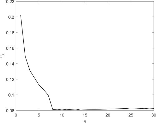
We first investigate the influence of the parameter η which appears in (5(5) ${\alpha }_k=\frac{k-1}{k+\eta },\eta \ge -1.$(5) ).For fixed noise level $ϵ=0.01$, the relation between relative error $e_k$ and η is plotted in Figure 1, which indicate that, in general, the value of η should not be selected too small, this is consistent with our theoretical results. In practical application, the parameter η is always selected as small as possible. Therefore in the following numerical experiments, we always choose $\eta =4$.

Figure 1. Example 1: the relative error $e_k$ versus η with noise level $ϵ=0.01$.

In Figure 2, we present the behaviour of residuals and relative errors with respect to the number of iteration steps using the noisy data ${\varphi }^{\delta }$ with noise level $ϵ=0.01$. We can see that the residuals corresponding to both the two methods decrease as k increase and the relative errors decrease first and then increase after several iteration steps, which indicate that choosing the appropriate number of stop iteration steps is very important for both methods. In the following, we take the regularization parameters based on (22(22) $\Vert A{f}_{\rho }^{k^{\ast },\delta }-{\varphi }_{\rho }^{\delta }{\Vert }_{\rho }\le \tau \delta <\Vert A{f}_{\rho }^{k,\delta }-{\varphi }_{\rho }^{\delta }{\Vert }_{\rho },0\le k<k^{\ast },$(22) ) with $\tau =1.1$. The comparisons between the exact source function and the reconstructed solution obtained by both the original method (34(34) $f^{k+1,\delta }=f^{k,\delta }-\text{β}(K{f}^{k,\delta }-{\varphi }^{\delta }),k=0,1,\dots$(34) ) and the accelerated method (35(35) $\begin{array}{rl}& z^{k,\delta }=f^{k,\delta }+{\alpha }_k(f^{k,\delta }-f^{k-1,\delta }),\\ & f^{k+1,\delta }=z^{k,\delta }-\text{β}(K{z}^{k,\delta }-{\varphi }^{\delta }),k=0,1,\dots \end{array}$(35) ) are presented in Figure 3. From Figure 3, it can be seen that, both the original method (34(34) $f^{k+1,\delta }=f^{k,\delta }-\text{β}(K{f}^{k,\delta }-{\varphi }^{\delta }),k=0,1,\dots$(34) ) and the accelerated method (35(35) $\begin{array}{rl}& z^{k,\delta }=f^{k,\delta }+{\alpha }_k(f^{k,\delta }-f^{k-1,\delta }),\\ & f^{k+1,\delta }=z^{k,\delta }-\text{β}(K{z}^{k,\delta }-{\varphi }^{\delta }),k=0,1,\dots \end{array}$(35) ) can give satisfactory reconstruction results for different noise levels, but the required number of iteration steps and the computation time for the accelerated method are much less than that of the original method (see Table 1).

Figure 2. Example 1: (a) the residual $E_k$ versus k ; (b) the relative error $e_k$ versus k.

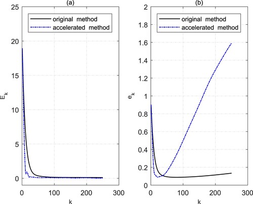
Figure 3. Example 1: (a)–(c) The reconstructed source function obtained by the original method; (d)–(f) The reconstructed source function obtained by the accelerated method.

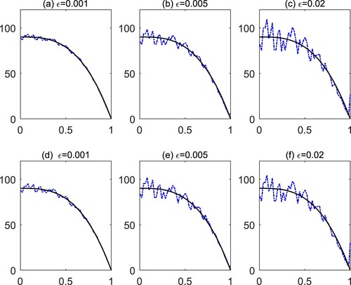
Table 1. Numerical comparison on the original method and the accelerated method for Example 3.1.

	Original method			Accelerated method
ϵ	$k^{†}$	$e_{k^{†}}$	CPU time(s)	$k^{\ast }$	$e_{k^{\ast }}$	CPU time(s)
0.0001	680	0.0041	229.34	124	0.0075	41.74
0.0005	371	0.0110	127.59	67	0.0140	23.54
0.001	286	0.0172	100.37	63	0.0250	21.96
0.005	158	0.0513	58.78	42	0.0638	15.11
0.01	118	0.0835	43.93	41	0.1218	15.33
0.02	82	0.1357	31.06	22	0.1333	7.94

Example 3.2

In this example, we consider the oscillating source function $f\left(\rho \right)=5(1+\cos (5\pi \rho \left)\right)$ over the interval $[0,1]$. The obtained numerical results are shown in Figure 4 and Table 2. It is observed that, for this oscillating function, more iteration steps are needed to satisfy the discrepancy principle (22(22) $\Vert A{f}_{\rho }^{k^{\ast },\delta }-{\varphi }_{\rho }^{\delta }{\Vert }_{\rho }\le \tau \delta <\Vert A{f}_{\rho }^{k,\delta }-{\varphi }_{\rho }^{\delta }{\Vert }_{\rho },0\le k<k^{\ast },$(22) ). Table 2 further confirms that both the methods perform well although the number of iteration steps and computation time required by the accelerated method (35(35) $\begin{array}{rl}& z^{k,\delta }=f^{k,\delta }+{\alpha }_k(f^{k,\delta }-f^{k-1,\delta }),\\ & f^{k+1,\delta }=z^{k,\delta }-\text{β}(K{z}^{k,\delta }-{\varphi }^{\delta }),k=0,1,\dots \end{array}$(35) ) are far less than that of the original method (34(34) $f^{k+1,\delta }=f^{k,\delta }-\text{β}(K{f}^{k,\delta }-{\varphi }^{\delta }),k=0,1,\dots$(34) ).

Figure 4. Example 2: (a)–(c) The reconstructed source function obtained by the original method; (d)–(f) the reconstructed source function obtained by the accelerated method.

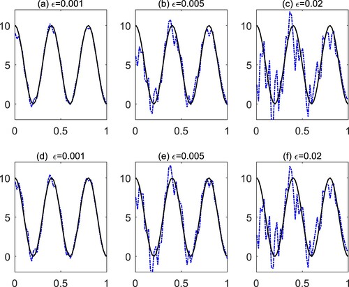
Table 2. Numerical comparison on the original method and the accelerated method for Example 3.2.

	Original method			Accelerated method
ϵ	$k^{†}$	$e_{k^{†}}$	CPU time(s)	$k^{\ast }$	$e_{k^{\ast }}$	CPU time(s)
0.0001	2568	0.0093	826.13	322	0.0154	102.73
0.0005	1487	0.0275	476.02	200	0.0547	63.90
0.001	1173	0.0452	377.27	130	0.0631	41.46
0.005	610	0.1334	199.12	82	0.1551	26.26
0.01	443	0.2006	145.66	61	0.1955	19.33
0.02	316	0.2927	104.66	47	0.2619	14.89

Example 3.3

In this example, we consider the source function $f\left(\rho \right)=\{\begin{array}{cl}1,& 0\le \rho <0.5,\\ 16(1-\rho {)}^4,& 0.5\le \rho \le 1.\end{array}$ This is a more difficult example since the function is not smooth at the point $\rho =0.5$. Figure 5 shows the comparisons between the exact source function and the reconstructed solution obtained by both the original method (34(34) $f^{k+1,\delta }=f^{k,\delta }-\text{β}(K{f}^{k,\delta }-{\varphi }^{\delta }),k=0,1,\dots$(34) ) and the accelerated method (35(35) $\begin{array}{rl}& z^{k,\delta }=f^{k,\delta }+{\alpha }_k(f^{k,\delta }-f^{k-1,\delta }),\\ & f^{k+1,\delta }=z^{k,\delta }-\text{β}(K{z}^{k,\delta }-{\varphi }^{\delta }),k=0,1,\dots \end{array}$(35) ). Further numerical results are shown in Table 3. These numerical results are very similar to that in the Example 3.1 and 3.2. Particularly, from Figure 5 and Table 3, we can see that even for this nonsmooth function the accelerated method (35(35) $\begin{array}{rl}& z^{k,\delta }=f^{k,\delta }+{\alpha }_k(f^{k,\delta }-f^{k-1,\delta }),\\ & f^{k+1,\delta }=z^{k,\delta }-\text{β}(K{z}^{k,\delta }-{\varphi }^{\delta }),k=0,1,\dots \end{array}$(35) ) still works well with fewer iteration steps.

Figure 5. Example 3: (a)–(c) The reconstructed source function obtained by the original method; (d)–(f) the reconstructed source function obtained by the accelerated method.

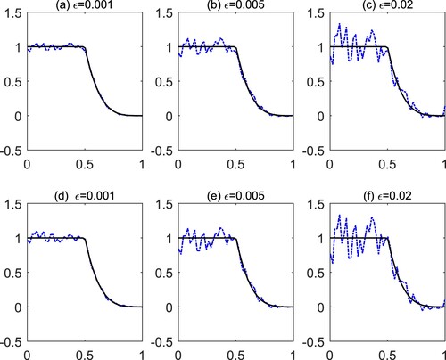
Table 3. Numerical comparison on the original method and the accelerated method for Example 3.3.

	Original method			Accelerated method
ϵ	$k^{†}$	$e_{k^{†}}$	CPU time(s)	$k^{\ast }$	$e_{k^{\ast }}$	CPU time(s)
0.0001	2234	0.0110	591.22	212	0.0135	55.73
0.0005	966	0.0227	256.39	122	0.0280	31.76
0.001	674	0.0329	177.44	96	0.0402	25.34
0.005	290	0.0770	78.46	59	0.0955	16.07
0.01	214	0.1134	59.08	42	0.1126	11.34
0.02	158	0.1717	44.71	39	0.1911	10.91

4. Conclusion

In this work, we consider an inverse radiogenic source problem associated to the helium production-diffusion equation. A fast iterative method has been proposed to solve the inverse source problem. Both the a priori and a posteriori regularization parameter choice rules were investigated for the proposed method. Furthermore, the convergence rates were provided for the regularized solutions generated by the iterative regularization method. Numerical results indicate that the proposed method is efficient, accurate and stable to compute the approximation of the unknown radiogenic source.

We conclude the paper by some remarks. In this paper, although our theoretical analysis is based on the eigenfunction expansion, our numerical experiments do not depend on the eigenvalues and eigenfunctions at all. In each step, we only need to numerically solve a forward problem. So our method can be easily extended to the problem for general geometry, which will be considered in the future.

Disclosure statement

No potential conflict of interest was reported by the author(s).

Additional information

Funding

The research of Z Zhang is partially supported by the NSF of China [grant number 12171215,11601207] and NSF of Gansu Province [grant number 21JR7RA475]. The research of Y Zhang is partially supported by the NSF of China [grant number 11871392] and the Fundamental Research Funds for the Central Universities [grant number lzujbky-2020-12].

References

- Choulli M, Yamamoto M. Conditional stability in determining a heat source. J Inverse Ill-posed Probl. 2004;12(3):233–243.
- Hettlich F, Rundell W. Identification of a discontinuous source in the heat equation. Inverse Probl. 2001;17(5):1465.
- Sakamoto K, Yamamoto M. Inverse heat source problem from time distributing overdetermination. Appl Anal. 2009;88(5):735–748.
- Dou FF, Fu CL, Yang F. Identifying an unknown source term in a heat equation. Inverse Probl Sci Eng. 2009;17(7):901–913.
- Hussein MS, Lesnic D, Johansson BT, et al. Identification of a multi-dimensional space-dependent heat source from boundary data. Appl Math Model. 2018;54:202–220.
- Johansson T, Lesnic D. Determination of a spacewise dependent heat source. J Comput Appl Math. 2007;209(1):66–80.
- Xie J, Zou J. Numerical reconstruction of heat fluxes. SIAM J Numer Anal. 2005;43(4):1504–1535.
- Yan L, Fu CL, Dou FF. A computational method for identifying a spacewise-dependent heat source. Int J Numer Method Biomed Eng. 2010;26(5):597–608.
- Yang F, Fu CL. The revised generalized Tikhonov regularization for the inverse time-dependent heat source problem. J Appl Math Comput. 2013;41(1–2):81–98.
- Bao G, Dou Y, Ehlers T, et al. Quantifying tectonic and geomorphic interpretations of thermochronometer data with inverse problem theory. Commun Comput Phys. 2011;9(1):129–146.
- Bao G, Ehlers TA, Li P. Radiogenic source identification for the helium production-diffusion equation. Commun Comput Phys. 2013;14(1):1–20.
- Shuster DL, Farley KA. 4he/3he thermochronometry: theory, practice, and potential complications. Rev Mineral Geochem. 2005;58(1):181–203.
- Wolf RA, Farley KA, Kass DM. Modeling of the temperature sensitivity of the apatite (ucth)/he thermochronometer. Chem Geol. 1998;148(1):105–114.
- Zhang YX, Yan L. The general a posteriori truncation method and its application to radiogenic source identification for the helium production–diffusion equation. Appl Math Model. 2017;43:126–138.
- Geng X, Cheng H, Liu M. Inverse source problem of heat conduction equation with time-dependent diffusivity on a spherical symmetric domain. Inverse Probl Sci Eng. 2021;29(11):1–16.
- Deng Y, Liu Z. Iteration methods on sideways parabolic equations. Inverse Probl. 2009;25(9):Article ID 095004, 14pp.
- Wang J-G, Wei T. An iterative method for backward time-fractional diffusion problem. Numer Methods Partial Differ Equ. 2014;30(6):2029–2041.
- Wang JG, Ran YH. An iterative method for an inverse source problem of time-fractional diffusion equation. Inverse Probl Sci Eng. 2018;26(10):1–13.
- Kindermann S. Optimal-order convergence of Nesterov acceleration for linear ill-posed problems. Inverse Probl. 2021;37(6):Article ID 065002, 21pp.
- Neubauer A. On Nesterov acceleration for Landweber iteration of linear ill-posed problems. J Inverse Ill-posed Probl. 2017;25(3):381–390.
- Watson GN. A treatise on the theory of Bessel functions. Cambridge: Cambridge University Press; 1995.
- Engl HW, Hanke M, Neubauer A. Regularization of inverse problems. Dordrecht: Kluwer Academic Publishers Group; 1996.
- Lai MC, Wang WC. Fast direct solvers for Poisson equation on 2d polar and spherical geometries. Numer Methods Partial Differ Equ: An Int J. 2002;18(1):56–68.
- Schiesser WE, Griffiths GW. A compendium of partial differential equation models: method of lines analysis with matlab. Cambridge: Cambridge University Press; 2009.