
 ?Mathematical formulae have been encoded as MathML and are displayed in this HTML version using MathJax in order to improve their display. Uncheck the box to turn MathJax off. This feature requires Javascript. Click on a formula to zoom.
ABSTRACT
We study the Phase Retrieval (PR) problem under the phaseless short-time Fourier transform (STFT) measurements. This paper proposes a novel algorithm named PAR to solve the STFT PR problem in phase and amplitude respectively with a milder retrieval condition compared with the original methods. First, a symmetric undirected graph of signals is proposed for the computation of the relative phase. Then the retrieval conditions of STFT PR problem are discussed for a single window case and some weaker retrieval conditions are proposed compared with the LS method. We also discuss STFT PR problem in multiple windows and establish retrieval theorems without restrictions of sliding step-size L. We give some numerical results of the PAR algorithm.
MSC:
1. Introduction and problem equation
Phase Retrieval(PR) is a classical problem which considers recovering a signal from the magnitude of the measurements. It can be applied in X-ray crystallography [Citation1,Citation2], diffraction imaging system [Citation3], phase measurement in astronomy [Citation4,Citation5] and optics [Citation6,Citation7]. When the phase retrieval measuring vectors are chosen as Short Time Fourier Transform(STFT) measurements [Citation6], it is an STFT PR problem. This problem serves as the model for ptychography, in which one or multiple moving probes are used to sense multiple diffraction measurements [Citation8,Citation9] and ultra-short laser pulse measurement techniques [Citation10,Citation11]. Different number of probes and laser pulses corresponds single or multiple STFT PR problem [Citation12,Citation13].
This paper considers the STFT phase retrieval, which recovering a signal from its STFT magnitude. Set The STFT can be interpreted as the Fourier transform of an N-dimensional signal
multiplied by series of sliding windows
with N-periodic extension:
(1)
(1)
with
,
and
. m represents the sliding order of the window
and L represents the sliding step-size. STFT PR considers the problem of recovering
from
. When R = 1, the problem is a single STFT phase retrieval problem, while R>1 is a multiple STFT phase retrieval problem [Citation14,Citation15].
To solve STFT PR, not only the algorithm but also retrieval conditions need to be considered. It means the conditions under which the STFT magnitude uniquely identifies signals (up to a global phase) [Citation16] under the algorithm. Researchers find that a suitable restriction of measurements including windows' number, type, length and step size enforce retrieval uniqueness.
For single STFT PR problem, different algorithms have various restrictions of windows. Denote the length nonzero window by W. When the measurement is with adjacent windows (L = 1), SDP approach [Citation17] has been extended to STFT PR [Citation18] and has uniqueness guarantees with computational complexity
. When the sliding step-size L = 1 and
, a Least Squares (LS) approach [Citation19] obtains the stable solution of STFT PR. In addition, a robust method proposed in [Citation20] uses phase polarization to solve STFT PR under a sliding window with length W = N, which is too restrictive in many applications.
As for multiple PR, [Citation14] discusses some sufficient and necessary conditions of multi-windows STFT PR and an algorithm based on the graph was proposed to recover the signal. But this retrieval condition is quite special () and can only be satisfied in strict conditions. Greedy Angular Synchronization [Citation21–23] is proposed to compute relative phase by autocorrelation. While it assumes that all the autocorrelation.
can be obtained for all
where δ is a given length, it may not easy to satisfy this condition in STFT PR problem.
No matter for single or multiple windows STFT PR, those algorithms have special retrieval restrictions of measurements, which restrict the applications. A better algorithm should consider the retrieval conditions and be suitable for broader applications. In this paper, an algorithm named PAR, which compute phase and amplitude respectively (PAR), is proposed with a milder retrieval restrictions of measurements for both single and multiple STFT PR. First, a graph is established based on STFT measurements and the retrieval conditions of PAR are transformed to the graph connectivity. Based on the analysis of the graph connectivity, some milder retrieval conditions are proposed for different types of windows, which has a broader field of application. Error estimation and experiments are also given to verify the effectiveness of the PAR algorithm.
Throughout the paper, we use the following notation. Bold-face small and capital letters denote vectors and matrices respectively. denotes the greatest common factor between a, b and c.
denotes 1D discrete Fourier transform (DFT) and
denotes 1D discrete inverse Fourier transform (IDFT).
is defined as
(2)
(2)
and
is defined as
(3)
(3)
The paper is organized as follows. In Section 1, we introduce the STFT PR problem and related works. Section 2 discusses the PR problem in the single-window and multi-window respectively. Section 3 gives the reconstruction algorithm and error estimation. Section 4 compares the numerical results of PAR and LS method. Section 5 is the summary of this paper.
2. Analysis of phase retrieval conditions
Define . Instead of recovering x from
, this paper considers the acquired data
by taking IDFT of
for
, which is defined as
(4)
(4)
with
,
[Citation19]. Therefore, recovering
from
is equivalent to recover it from
. To recover the signal
uniquely, the injectivity property of
should be guaranteed. Actually, there are classes of signals that have the same measurements after injection. For arbitrary
,
and
produce the same intensity measurements. Thus we consider
and
as in the same class
, where ∼ is the equivalence relation of being identical up to a global phase factor. Then the distance between two vectors in
is defined as
(5)
(5)
When
,
and
are equivalent up to a global phase shift.
2.1. Single adjacent window case (R = 1, L = 1)
To find the relation between success of recovery and windows' parameters, we first discuss the STFT PR problem with a single window . Denote
and
. Then Equation (Equation4
(4)
(4) ) can be represented by
(6)
(6)
Define
,
, and matrix
, where the
entry of
is equal to
. Then Equation (Equation6
(6)
(6) ) can be written as
(7)
(7)
Due to L = 1,
is a circulant square matrix which can be diagonalized by
, where
is a diagonal matrix whose entries are given by the DFT of the first column of
.
is the DFT matrix and
represents the conjugate transpose matrix of
[Citation24]. If the matrices
are invertible for several
, then we can compute
by
(8)
(8)
To analyse the invertibility of
, the definition of ‘non-vanishing’ is given as follows:
Definition 2.1
is non-vanishing means
for all
.
Denote .
is invertible if and only if
is non-vanishing since
. Based on this, LS algorithm proposed in [Citation19] can be used to solve the PR problem when
is non-vanishing for
. Nevertheless, Theorem 3.3 in [Citation19] shows that if
is non-vanishing only for l = 0, 1, signal can still be recovered. It inspires us to consider recovering the signal under milder and wider conditions.
Suppose signal is non-vanishing. In fact, for any
and
, since
and
are in the same class of
, we do not need to compute all the phase, but the relative phase [Citation6]:
(9)
(9)
To compute the signal phase, we define an undirected graph for STFT phase retrieval:
(10)
(10)
with a set of nodes:
and a set of edges:
Relative phase information can be transferred through the relationship between the phase of
:
(11)
(11)
If we assign an arbitrary nonzero vertex
to have nonzero phase
, then all the phase can be computed due to phase propagation equation (Equation11
(11)
(11) ) if graph G is connected. In this paper, we can use the same strategy as [Citation23] to choose the initial phase
. Therefore, the graph connectivity decides the retrieval uniqueness of phase.
Lemma 2.1
If there exists non-vanishing , then
can be computed by the phase of
for any
.
Proof.
According to Equations (Equation8(8)
(8) ) and (Equation9
(9)
(9) ),
can be computed when
is invertible, which is equivalent to
is non-vanishing.
Since the STFT of signal is periodic, the connectivity of graph G is related to l and N. We have the following results:
Lemma 2.2
Given a graph G with N vertices, suppose there exists k such that any two vertices and
are connected if and only if
, then graph G is connected if and only if
.
Proof.
Graph connectivity can be judged by the adjacency matrix . If all the elements in
are non-zero, graph is connected. The adjacency matrix of G is in this form
(12)
(12)
(13)
(13)
It shows that
and
for
. Since
, then all elements in S are non-zero is equivalent to that
for
covers all the position in matrix A, which means that
A generalized result of Lemma 2.2 is given by Lemma 2.3.
Lemma 2.3
Given a graph G with N vertices, suppose any two vertices and
are connected if
for
. G is connected if and only if
.
Proof.
The lemma can be inferred by S defined in Lemma 2.2. Denote the adjacency matrix is A, then and
for
and
. Only when
, all elements in S are non-zero.
Lemmas 2.2 and 2.3 give the relation between k and N. Combining with Lemma 2.1, we get two theorems as follows:
Theorem 2.4
Assume there exists , such that
and
is non-vanishing, then all phases can be recovered.
Theorem 2.5
Assume there exists such that
, and
is non-vanishing for
, then the phase can be recovered.
Proof.
Since is non-vanishing,
can be computed, which means the relative phase between
and
can be obtained. According to Lemma 2.2 and 2.3, all phases can be computed.
Theorem 2.4 and 2.5 give two phase recovery conditions. Then we turn to consider how to compute the amplitude. As is shown in Theorem 3.1 in [Citation19] and Algorithm 1 in [Citation23], the amplitude can be computed when is non-vanishing. However, if
is vanishing, could signal
still be recovered? Here we make an extension of proposition III.4 in [Citation19].
Theorem 2.6
If there exists such that
where
, and
,
are both non-vanishing, then the amplitude of the signal
can be recovered by
(14)
(14)
Proof.
Without loss of generality, since , then
(15)
(15)
We could compute the amplitude of
and other vertices amplitude can be computed by the same equation.
Remark 2.1
Since Equation (2.6) involves division, the signal should be non-vanishing and not too small. Here is an example. If and
are both non-vanishing, then
(16)
(16)
Other vertices can also be computed by this equation.
Corollary 2.7
If there exists such that
and
are non-vanishing, then the signal can be recovered.
Proof.
Since for any integer
, then all phases can be computed according to Theorem 2.4. And it also ensures the amplitude can be computed by Theorem 2.6. Therefore, the signal can be recovered.
Remark 2.2
Corollary 2.7 gives a sufficient condition for the recovery of . Theorem III.4 proposed in [Citation19] is a special case of Corollary 2.7.
Now we can prove that when , our method can also recover the phase, which expands the scope of W compared with LS model.
Corollary 2.8
If and
, then the signal phase can be recovered.
Proof.
Consider the matrix where the
th entry of
is given by
. Since
and
, there must exist unique
such that
. Therefore, we have
(17)
(17)
Since
,
(18)
(18)
Then
can be computed as
Since m is arbitrary, for any
and
,
can be computed if
. Therefore, there exists k = W so that
can be computed for
. Together with
, the signal phase can be recovered according to Lemma 2.2 where k = W.
By now, the discussion is based on L = 1. We now extend the results to L>1. In fact, since defined in (Equation7
(7)
(7) ) is not invertible,
cannot be computed by (Equation8
(8)
(8) ) for
. The problem is in that condition the graph G defined in (Equation10
(10)
(10) ) cannot be connected if there is only one l satisfy conditions of Theorem 2.4 when L>1. Therefore, we discuss multiple windows STFT to solve the conditions that
.
2.2. Multiple discrete windows case ( )
)
Multiple windows STFT PR provides more measurements compared with single window STFT PR. Therefore, the graph connectivity of G may be easier to satisfy.
Now we start to figure out which condition should be satisfied to ensure graph G is connected in STFT PR problem. Choose a window such that
. When
, there exists unique
such that
, then
Therefore,
(19)
(19)
Note that only when
with
,
can be computed by Equation (Equation19
(19)
(19) ). Therefore, single window STFT measurements cannot satisfy the connection of graph
when L>1. If we want to compute all the relative phase in the
, multiple windows
are needed to compute the relative phase. As an instance shown in Figure , when N = 6, L = 2,
,
, the graph G is connected.
Figure 1. An example of connected graph with two sliding windows:
,
.
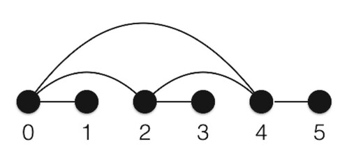
In this example, all the relative phase can be computed through (Equation19(19)
(19) ). It shows that when L>1, the relative phase still can be obtained. Given two vertices
and
, we want to figure out in which condition
can be computed. Based on Theorem 2.4, we get some conclusions in multiple windows. Based on Equation (Equation7
(7)
(7) ) and the solution identification theorem in linear equations, we get
Lemma 2.9
Denote the of
in Equation (Equation7
(7)
(7) ) as
,
. Let
. Then
can be computed by
if
.
Based on Lemma 2.9, Theorem 2.10 gives an extension of Theorem 3.1 in [Citation19] and Lemma 2.1.
Theorem 2.10
Let be a family of sliding windows with the same sliding step-size L, where L be a separation parameter with
. Define
, where
.
can be computed if
has rank L for all
.
Proof.
Since with
and
. Denote
, according to Fourier convolution property, we have
Denote
. Since
and
. Then according to Fourier transform property, for
and
,
(20)
(20)
Based on the equation of Lemma III.17 in [Citation14], we get
where
for all
and
.
Thus together with ,
(21)
(21)
Then
can be computed by the phase of
. Since
is invertible for all m, l, which means
, then we finished the proof.
Remark 2.3
Now consider some special cases of the condition given by Theorem 2.10.
When L = 1,
When L = N,
Based on Theorem 2.10, we can get theorems as follows:
Theorem 2.11
Suppose there exists so that
, and
has rank L for
, then the signal phase can be recovered.
Theorem 2.12
If there exists such that
,
and
have rank L, then the amplitude of the signal can be recovered.
Proof.
According to Theorem 2.10, if has rank L,
can be computed by Equation (Equation21
(21)
(21) ). Thus Theorem 2.11 and 2.12 can be inferred based on Theorems 2.5 and 2.6.
3. Reconstruction and error estimation
Theorems 2.11 and 2.12 extend retrieval conditions from a single window to multiple windows
, and the sliding size L = 1 to L>1. Based on these analyses, we propose the following reconstruction algorithm (PAR).
Here we discuss the computation complexity of PAR algorithm. To finish calculating and
, we can use fast Fourier transforms with
. Computing the rank of
needs
operations, while computing the highest common factor of no more than N number needs
by division algorithm in Theorem 2.11. Assume the number of l meeting conditions in Theorem 2.11 is k, then judging the condition of Theorem 2.12 needs at most
. According to Equations (Equation21
(21)
(21) ) and (Equation14
(14)
(14) ), computing relative phase and amplitude needs
respectively. Thus the total runtime complexity of PAR algorithm is
in general.
Based on our phase retrieval procedure, we now present the following guarantee of stable performance. Suppose the measurements are corrupted by random noise with level
according to Equation (Equation4
(4)
(4) ), then the problem become recovering the signal
from
. For a window family
with period N extension, we define
,
,
Theorem 3.1
Let ,
. Denote
,
, where
,
and M are defined in Equation (Equation14
(14)
(14) ) and Algorithm 1. Let
be the approximation obtained by Algorithm 1 from noisy measurements
,
then there exists
such that for all
,
(22)
(22)
and
(23)
(23)
Proof.
For any ,
The last inequality comes from Cauchy–Schwarz inequality. Denote
is the IDFT of
in (Equation4
(4)
(4) ). Combine with Equation (Equation21
(21)
(21) ), then we get
(24)
(24)
According to the error transfer formula: If
, then error estimation
(25)
(25)
where
represent the error bound of each variable.
(26)
(26)
Then according the triangle inequality, we get that
(27)
(27)
Since the relative phase propagation in graph G, we have the estimation equation (Equation22
(22)
(22) ).
Let be the vectors of phases of the entries of
and
. ° represents Hadamard product. The reconstruction error
(28)
(28)
Theorem 3.1 ensures that when error ε is in low level and the minimal of
is not small, the error between retrieval phase and exact phase can be controlled. In addition, the norm of
and
influences the upper bound of error. Therefore, the number of windows does not need to be too large but should meet the retrieval conditions. It means that if we choose some suitable windows, the signal can be recovered well by PAR.
4. Numerical results
We now show the results of PAR algorithm in different types of signals and sliding windows. Here we choose three different signals, Gaussian complex signal, chirp signal and real temperature signal. A Gauss complex signal with N = 101, which is defined as
(29)
(29)
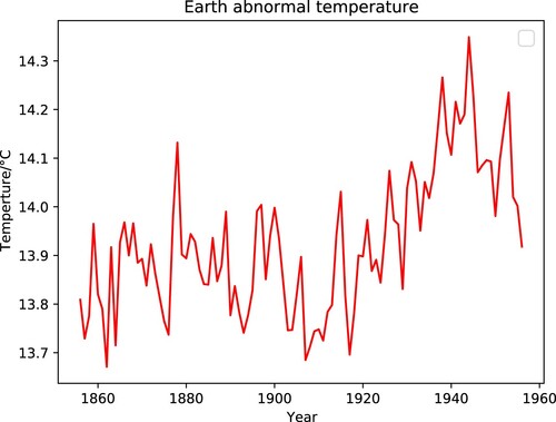
Chirp signal is a typical non-stationary signal in communication, sonar, radar. Figure shows a chirp signal with length N = 101 and average value is 0. Earth abnormal temperature signal is a real signal describing the temperature variation in Figure .
Figure 2. Chirp signal.
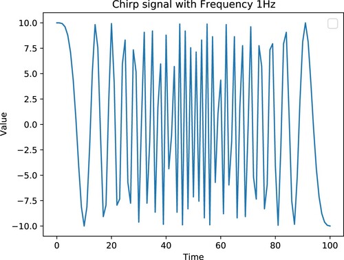
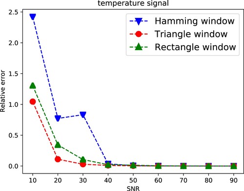
Figure 3. Earth abnormal temperature.
In addition, we choose some different typical sliding windows in STFT including rectangle windows, triangle windows and hamming windows. These windows have different main lobes and side lobes, which are suitable for different situations. All the sliding windows satisfy the retrieval condition in PAR method. These simulations display the relation between relative error and sliding window as well as signal-noise ratio (SNR), where the relative error between estimation and real signal
is defined as
We reproduce our procedure in https://github.com/zhouxianchen/PAR-algorithm with python.
4.1. Relative error and length of window
Since LS method in [Citation19] requires , we first discuss the relationship between relative error and sliding window with two signals. Here we choose parameter
and
in (Equation29
(29)
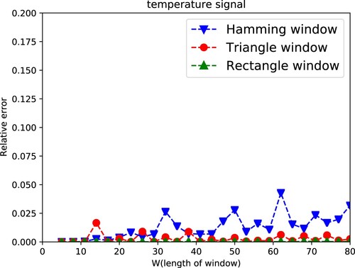
(29) ). Figure and Figure show PAR method has less than 0.025 relative error without considering the length of window W in three types of windows. And two figures show that PAR method has no restriction with length of window and can be used in wider range compared with the LS method. Relative error in chirp signal and temperature signal is relatively smaller than that in Gauss complex signal, which might be because that it is no relative phase error in the reconstruction procedure with real signal (Figure ).
Figure 4. Relative error in recovering Gaussian complex signal by different windows using PAR.
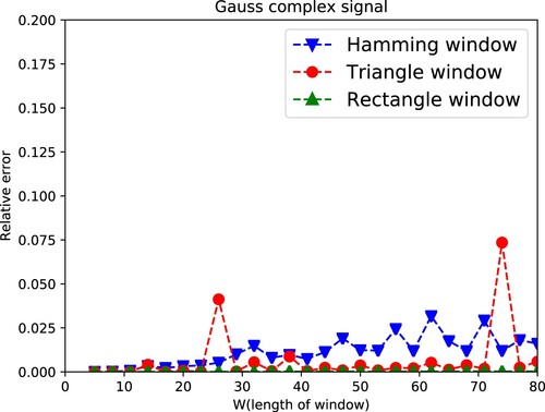
Figure 5. Relative error in recovering chirp signal by different windows using PAR.
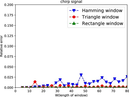
Figure 6. Relative error in recovering temperature signal by different windows using PAR.
4.2. Relative error and SNR
Here we discuss PAR performance in different SNR. We choose the length of window W = 7 and in (Equation29
(29)
(29) ). Figure shows that PAR can retrieve signal when
. When
, different windows have different performance in the same level SNR. The triangle window has better performance compared with rectangle and hamming windows. We infer it is due to that
and
in (Equation22
(22)
(22) ) are influenced by the type of windows, which lead to different error estimation (Figures and ).
Figure 7. Relative error in recovering noisy Gaussian signal using PAR (W = 7).
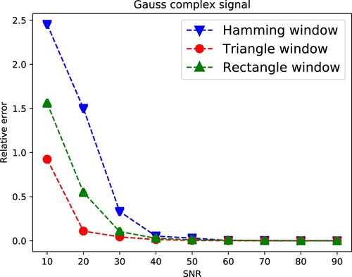
Figure 8. Relative error in recovering noisy chirp signal using PAR (W = 7).
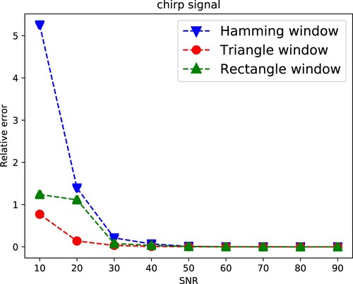
Figure 9. Relative error in recovering temperature signal using PAR (W = 7).
4.3. Relative error and μ
To verify our error estimation, we discuss the relationship between relative error and μ in (Equation29(29)
(29) ) using a Gauss complex signal. Here we choose a Hamming window STFT. Figure shows that when
,
can retrieve signal correctly. And when
is larger, PAR method has robuster retrieval performance. It verifies our error estimation formula (Equation22
(22)
(22) ) and inspires us when we deal with some data in reality, we can use a signal translation to enlarge that
(Figure ).
Figure 10. Relative error in recovering noisy Gaussian signal using PAR in different μ.
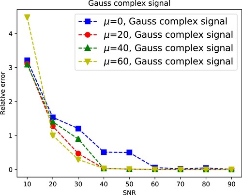
Figure 11. Relative error in recovering Gauss complex signal with Hamming window using PAR and LS method (SNR=100).
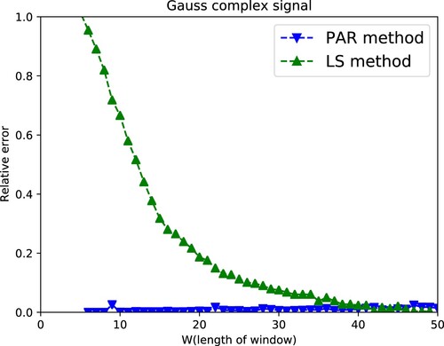
4.4. Relative error between LS and PAR algorithm
In this section, we display the performance of PAR algorithm and the classical LS [Citation19] algorithm under different length of window. PAR method has good performance when the length of W is small compared with the LS method. Therefore, PAR method has less restriction of the window length than the LS method.
As is shown in the experiments, no matter for Gaussian complex, chirp or real temperature signal, our method obtains better performance than the LS method. However, note that the retrieval conditions of PAR based on the assumption that the signal is non-vanishing and graph connectivity based on windows. Some signals and windows do not satisfy these assumptions, and our method is not suitable for those situations.
5. Conclusion and further work
Previous research proposed STFT PR methods in relatively strict retrieval conditions. This paper proposes a PAR reconstruction algorithm with a milder retrieval conditions, which solved the PR by computing phase and amplitude respectively. Compared with the previous method, PAR reconstruction Algorithm 1 has a milder constraint of windows and can be used to solve the STFT phase retrieval problems both in single window and multiple windows cases, when prior knowledge is known including that the noise is low and the minimal magnitude of nonzero components of original signal is enough large. Numerical results show that when noise is in low level, PAR has better performance and a translation shift of initial signal can lead to a robuster result. In addition, since the computation cost is when l is selected in Algorithm 1, it can also be used in initialization of other non-convex method.
Disclosure statement
There are no relevant financial or non-financial competing interests to report. And no potential competing interest was reported by the authors.
Additional information
Funding
References
- Harrison RW. Phase problem in crystallography. J Opt Soc Amer A. 1993;10(5):1046–1055.
- Miao J, Ishikawa T, Shen Q, et al. Extending x-ray crystallography to allow the imaging of noncrystalline materials, cells, and single protein complexes. Annu Rev Phys Chem. 2008;59(1):387–410.
- Bunk O, Diaz A, Pfeiffer F, et al. Diffractive imaging for periodic samples: retrieving one-dimensional concentration profiles across microfluidic channels. Acta Crystallogr. 2007;63(4):306–314.
- Fienup C, Dainty J. Phase retrieval and image reconstruction for astronomy. Image Recovery: Theor Appl. 1987;231:275.
- Stepanova IE, Gudkova TV, Salnikov AM, et al. A new approach to analytical modeling of Mars's magnetic field. Appl Math Sci Eng. 2022;30(1):41–60.
- Walther A. The question of phase retrieval in optics. Optica Acta Int J Opt. 1963;10(1):41–49.
- Geng Y, Wen X, Tan J, et al. Noise-robust phase retrieval by optics path modulation with adaptive feedback. Opt Commun. 2022;515:128199.
- Fienup JR, Guizarsicairos M. Phase retrieval with transverse translation diversity: a nonlinear optimization approach. Opt Express. 2008;16(10):7264–7278.
- Maiden AM, Humphry MJ, Zhang F, et al. Superresolution imaging via ptychography. J Opt Soc Am A Opt Image Sci Vis. 2011;28(4):604–612.
- Trebino R, Guang Z, Zhu P, et al. The measurement of ultrashort laser pulses. 2018 2nd URSI Atlantic Radio Science Meeting (AT-RASC); IEEE; 2018. p. 1–3.
- Kane DJ. Principal components generalized projections: a review [invited]. J Opt Soc Am B. 2008;25(6):A120–A132.
- Lin W, Zhang R, Xu X, et al. Phaseless signal recovery from triple-window short-time Fourier measurements. Int J Phys Conf Ser. 2020;1617:012081. IOP Publishing.
- Grohs P, Liehr L, Rathmair M. Multi-window STFT phase retrieval: lattice uniqueness. Preprint 2022. Available from: arXiv:2207.10620.
- Li L, Cheng C, Han D, et al. Phase retrieval from multiple-window short-time Fourier measurements. IEEE Signal Process Lett. 2017;24(4):372–376.
- Guo Y, Wang A, Wang W. Multi-source phase retrieval from multi-channel phaseless STFT measurements. Signal Process. 2018;144:36–40.
- Grohs P, Koppensteiner S, Rathmair M. Phase retrieval: uniqueness and stability. SIAM Rev. 2020;62(2):301–350.
- Jaganathan K, Oymak S, Hassibi B. Sparse phase retrieval: uniqueness guarantees and recovery algorithms. IEEE J Sel Top Signal Process. 2017;10(4):770–781.
- Sun DL, Smith Iii JO. Estimating a signal from a magnitude spectrogram via convex optimization. arXiv. 2012;1209.2076. DOI:10.48550/arXiv.1209.2076
- Bendory T, Eldar YC. Non-convex phase retrieval from STFT measurements. IEEE Trans Inform Theor. 2018;64(99):1–1.
- Pfander GE, Salanevich P. Robust phase retrieval algorithm for time-frequency structured measurements. SIAM J Imaging Sci. 2019;12(2):736–761.
- Alexeev B, Bandeira AS, Fickus M, et al. Phase retrieval with polarization. SIAM J Imaging Sci. 2014;7(1):35–66.
- Iwen MA, Viswanathan A, Wang Y. Fast local correlation measurements. SIAM J Imaging Sci. 2016;9(4):1655–1688.
- Iwen MA, Preskitt B, Saab R, et al. Phase retrieval from local measurements: improved robustness via eigenvector-based angular synchronization. Appl Comput Harmon Anal. 2020;48:415–444
- Bendory T, Eldar YC. Phase retrieval from STFT measurements via non-convex optimization. 2017 IEEE International Conference on Acoustics, Speech and Signal Processing (ICASSP); 2017. p. 4770–4774.