Efficient iterative scheme for solving non-linear equations with engineering applications

ABSTRACT

A family of three-step optimal eighth-order iterative algorithm is developed in this paper in order to find single roots of nonlinear equations using the weight function technique. The newly proposed iterative methods of eight order convergence need three function evaluations and one first derivative evaluation that satisfies the Kung–Traub optimality conjecture in terms of computational cost per iteration (i.e.$2^{n-1}$). Furthermore, using the primary theorem that establishes the convergence order, the theoretical convergence properties of our schemes are thoroughly investigated. On several engineering applications, the performance and efficiency of our optimal iteration algorithms are examined to those of existing competitors. The new iterative schemes are more efficient than the existing methods in the literature, as illustrated by the basins of attraction, dynamical planes, efficiency, log of residual, and numerical test examples.

KEYWORDS:

• Numerical technique
• iterative methods
• computational time
• optimal order
• computational efficiency

MSC::

• 65-04
• 65H04
• 65H05
• 65H10
• 65H17

1 Introduction

The earliest problem in science, and primarily in mathematics, is finding the roots of nonlinear equation (1) $f\left(x\right)=0.$(1) Nonlinear equations are used in a broad variety of fields in science and engineering [1–3]. When real problems exist, such as weather forecasting, the correct placement of satellite systems in desired trajectories, earthquake magnitude estimation, and other advanced technical issues, only approximate techniques are frequently developed. Only in rare situations is it possible to solve the governing equations exactly. To determine the roots of nonlinear equation (1), several iterative approaches have been explored such as the Newton–Raphson method, decomposition methods, homotopy analysis method, and various modified forms of the Newton–Raphson method. The Newton–Raphson method [4] iterative scheme is the most well-known single root finding method: (2) $y_i=x_i-\frac{f\left(x_i\right)}{f^{\mathrm{\prime }}\left(x_i\right)},(i=1,2,\dots ),f^{\mathrm{\prime }}\left(x_i\right)\ne 0.$(2)

The method described by (2) has optimum convergence order 2 with efficiency $\mathrm{1.43.}$ Several higher order iterative algorithms for solving nonlinear equations have already been developed and researched in the past decade, namely Newton’s method, Chebyshev method, Halley’s iteration technique, and others see e.g. Wang et al. [6] present Modified Ostrowski’s method of eight-order convergence, Li et al. [7] proposed a higher order iterative method, Kung et al. [20] presented optimal order of one point and multipoint iterative schemes, Chicharro, et al. [28] illustrate the stability and applicability of iterative methods with memory, Zafar et al. [29] proposed efficient family of the iterative method of eight order convergence, Tao et al. [30] used divide difference techniques to construct optimal fourth- and eighth-order convergent scheme and Shacham et al. [31] proposed higher order improved memory methods for finding roots of non-linear equations. As the order of convergence increases, the number of function evaluations per iteration increases. As a result, a new performance criterion has emerged: efficiency, which indicates that any multi-point technique without memory that performs n function evaluations cannot have an order of convergence higher than 2${}^{n-1}$, which is the optimum order. Thus, for three evaluations per iteration, the optimal order is four, for four evaluations per iteration, eight, and so on. As a consequence, the overall aim of this study is to develop more efficient iterative schemes in comparison with existing methods in the literature. We developed a new iterative method to increase the order of convergence without increasing the functional evaluations. We can easily acquire the optimal order; as we will see, the obtained three-step method is of eighth-order convergence and takes four evaluations of the function $f\left(x\right)$. The efficiency of an iterative method is commonly analysed in the literature using the efficiency index $I\approx p^{\frac{1}{d}}$, where $p$ is the order of convergence and $d$ is the total number of functional evaluations or its derivative evaluations in each iteration. As a result, this technique has an efficiency index of $8^{\frac{1}{4}}\approx 1.6874$, indicating that it is the first to achieve the optimal order of convergence according to the Kung–Traub conjecture [20].

The weight function technique motivates us to propose a family of the eighth-order numerical iterative scheme for finding roots of (1). In [10–13,21–24], which use a variety of weight functions, how weight function processes can be applied is given. In this article, we employ the weight functions technique to construct a family of iterative algorithms with a high convergence order and efficiency index. Each iteration requires the evaluation of three functions and one first order derivative in terms of computational cost.

The conditions of Theorem 1.1 presented in this article are broad and fundamental for constructing an iterative technique for finding roots of nonlinear equations. Selecting functions that satisfy the theorem’s conditions is all that is required for a certain iterative technique. For example, one may write out the desired functions first, then use the theorem’s criterion to calculate the coefficients in the functions. Specific iterative techniques are illustrated in subsection (Concrete’s eight-order methods). The method’s attractiveness is because the developed scheme is directly applicable and requires the minimum number of functional evaluations available. Using a complex dynamical system, we choose the parameter values in the numerical scheme that yield the highest convergence rate. In terms of basins of attraction, we may compare our newly developed algorithms to a number of existing iterative techniques with the same convergence order and computational cost.

Here, we discuss some optimal eighth-order iterative methods for finding roots of nonlinear equations that exist in the literature.

The optimal eighth-order iterative method (abbreviated as MM1) due to Kung–Traub et al. [20] based on the Hermite interpolation is given by (3) $v_i=t_i-\frac{f\left(t_i\right)}{K\left(t_i\right)},$(3) where $y_i=x_i-\frac{f\left(x_i\right)}{f^{\mathrm{\prime }}\left(x_i\right)},$ $t_i=x_i-\frac{f\left(y_i\right)}{f^{\mathrm{\prime }}\left(x_i\right)}\left(\frac{1}{{\left(1-\frac{f\left(y_i\right)}{f\left(x_i\right)}\right)}^2}\right),$ $K\left(t_i\right)=2\left(f\left(x_i\right)-f\left[x_i,y_i\right]\right)+f[y_i,t_i]+\frac{y_i-t_i}{y_i-x_i}\left(f\left[x_i,y_i\right]-f^{\mathrm{\prime }}\left(x_i\right)\right).$

The following optimal eighth-order iterative approach was introduced by Babajee et al. [15] (abbreviated as MM2) (4) $v_i=t_i-\frac{f\left(t_i\right)}{f^{\mathrm{\prime }}\left(x_i\right)}\left(\frac{1+u^2+5u^4+v}{1-u-w}\right),$(4) where $y_i=x_i-\frac{f\left(x_i\right)}{f^{\mathrm{\prime }}\left(x_i\right)}{\left(1+\frac{f\left(x_i\right)}{f^{\mathrm{\prime }}\left(x_i\right)}\right)}^5,$ $t_i=y_i-\frac{f\left(y_i\right)}{f^{\mathrm{\prime }}\left(x_i\right)}\left(\frac{1}{{\left(1-u\right)}^2}\right),u=\frac{f\left(y_i\right)}{f\left(x_i\right)}$, $v=\frac{f\left(t_i\right)}{f\left(x_i\right)}$, $w=\frac{f\left(t_i\right)}{f\left(y_i\right)}.$

The optimal eighth-order iterative technique (abbreviated as MM3) given by Cordero et al. [16] is as follows: (5) $v_i=t_i-\frac{1-3w}{1+w}\frac{f\left(t_i\right)}{f[t_i,y_i]+f[t_i,x_i,x_i]\left(t_i-y_i\right)},$(5) where $y_i=x_i-\frac{f\left(x_i\right)}{f^{\mathrm{\prime }}\left(x_i\right)},$ $t_i=y_i-\frac{f\left(y_i\right)}{f^{\mathrm{\prime }}\left(x_i\right)}\left(\frac{1}{1-2u-u^2-\frac{u^3}{2}}\right),$ $f[t_i,x_i]=\frac{f\left(t_i\right)-f\left(x_i\right)}{t_i-x_i}$ and $f[t_i,x_i,x_i]=\frac{f[t_i,x_i]-f^{\mathrm{\prime }}\left(x\right)}{t_i-x_i}$.

Sharm’s family [17] of the optimal eighth-order method (abbreviated as MM4) is (6) $v_i=t_i-W\ast \left(\frac{f\left(t_i\right)f\left[x_i,y_i\right]}{f\left[x_i,t_i\right]f\left[y_i,t_i\right]}\right),$(6) where $y_i=x_i-\frac{f\left(x_i\right)}{f^{\mathrm{\prime }}\left(x_i\right)},$ $t_i=y_i-\frac{f\left(y_i\right)}{f^{\mathrm{\prime }}\left(y_i\right)}\left(\frac{1}{1-2u}\right),$ $W=1+\frac{w}{1+\alpha w}$ and $\alpha =1$.

Thukral [18] presented the following optimal eighth-order iterative method (abbreviated as MM5): (7) $v_i=t_i-\left[{\left(\frac{1-u^2}{1-u}\right)}^2-2u^2-6u^3+v+4w\right]\frac{f\left(t_i\right)}{f^{\mathrm{\prime }}\left(x_i\right)},$(7) where $y_i=x_i-\frac{f\left(x_i\right)}{f^{\mathrm{\prime }}\left(x_i\right)},$ $t_i=x_i-\frac{1}{f^{\mathrm{\prime }}\left(x_i\right)}\left(\frac{{\left(f\left(x_i\right)\right)}^2+{\left(f\left(y_i\right)\right)}^2}{\left(f\left(x_i\right)-f\left(y_i\right)\right)}\right),$ $u=\frac{f\left(y_i\right)}{f\left(x_i\right)}$, $v=\frac{f\left(t_i\right)}{f\left(x_i\right)}$, $w=\frac{f\left(t_i\right)}{f\left(y_i\right)}$.

Wang and Liu [19] presented Hermite interpolation based optimal eighth-order iterative method (abbreviated as MM6): (8) $v_i=t_i-\frac{f\left(t_i\right)}{f^{\mathrm{\prime }}\left(x_i\right)K\left(t_i\right)},$(8) where $y_i=x_i-\frac{f\left(x_i\right)}{f^{\mathrm{\prime }}\left(x_i\right)},$ $t_i=x_i-\frac{f\left(x_i\right)}{f^{\mathrm{\prime }}\left(x_i\right)}\left(\frac{4{\left(f\left(x_i\right)\right)}^2-5f\left(x_i\right)f\left(y_i\right)-{\left(f\left(y_i\right)\right)}^2}{\left(4{\left(f\left(x_i\right)\right)}^2-9f\left(x_i\right)f\left(y_i\right)\right)}\right),$ .$\frac{1}{K\left(t_i\right)}=\left(1+4\frac{f\left(t_i\right)}{f\left(x_i\right)}\right)\left(\frac{8f\left(y_i\right)}{4f\left(x_i\right)-11f\left(y_i\right)}+1+\frac{f\left(t_i\right)}{f\left(y_i\right)}\right)$

Liu and Wang’s [33] presented the following optimal eighth-order iterative method (abbreviated as MM7): (9) $v_i=t_i-\frac{f\left(t_i\right)}{f^{\mathrm{\prime }}\left(x_i\right)}\left({\left(\frac{f\left(x_i\right)-f\left(y_i\right)}{f\left(x_i\right)-2f\left(y_i\right)}\right)}^2+\left(\frac{f\left(t_i\right)}{f\left(y_i\right)-{\alpha }_{1}f\left(t_i\right)}\right)+\left(\frac{4f\left(t_i\right)}{f\left(x_i\right)+{\alpha }_{2}f\left(t_i\right)}\right)\right),$(9) where $y_i=x_i-{\displaystyle \frac{f\left(x_i\right)}{f^{\mathrm{\prime }}\left(x_i\right)}},$ $t_i=y_i-{\displaystyle \frac{f\left(y_i\right)}{f^{\mathrm{\prime }}\left(x_i\right)}}\left({\displaystyle \frac{f\left(x_i\right)}{f\left(x_i\right)-2f\left(y_i\right)}}\right)$ and α1, α2R.

Here, we proposed the following family of optimal eighth order methods: (10) $v_i=t_i-\frac{f\left(y_i\right)}{f^{\mathrm{\prime }}\left(x_i\right)}\left({\vartheta }_1\left(u\right){\vartheta }_2\left(v\right)+{\vartheta }_3\left(w\right){\vartheta }_3\left(w\right)+{\vartheta }_3\left(w\right){\vartheta }_2\left(v\right)\right),$(10) where $y_i=x_i-\frac{f\left(x_i\right)}{f^{\mathrm{\prime }}\left(x_i\right)},$ $t_i=y_i-\frac{f\left(y_i\right)}{f^{\mathrm{\prime }}\left(x_i\right)}\left(\frac{f\left(x_i\right)}{f\left(x_i\right)-2f\left(y_i\right)}\right),$ ${\vartheta }_1\left(u\right),{\vartheta }_2\left(v\right)$ and ${\vartheta }_3\left(w\right)$ are real-valued functions to be determined later on. For the iteration scheme (10), we have the following convergence theorem [11]:

Theorem 1.1:

Let $\zeta \in I$ be a simple root of a sufficiently differentiable function $f:I\subseteq R\to R$ in an open interval I. If $x_0$ is sufficiently close to $\zeta$ and $\vartheta$ be a real-valued function satisfying ${\vartheta }_1\left(0\right)=1,{\vartheta }_1^{\mathrm{\prime }}\left(0\right)=2,{\vartheta }_1^{\mathrm{\prime }\mathrm{\prime }}\left(0\right)=10,{\vartheta }_1^{\mathrm{\prime }\mathrm{\prime }\mathrm{\prime }}\left(0\right)=72,{\vartheta }_2\left(0\right)=1,$ ${\vartheta }_2^{\mathrm{\prime }}\left(0\right)=4,{\vartheta }_3\left(0\right)=0$, ${\vartheta }_3^{\mathrm{\prime }}\left(0\right)=1$ and ${\vartheta }_1^{\mathrm{\prime }\mathrm{\prime }\mathrm{\prime }\mathrm{\prime }}\left(0\right)={\vartheta }_2^{\mathrm{\prime }\mathrm{\prime }}\left(0\right)={\vartheta }_3^{\mathrm{\prime }\mathrm{\prime }}\left(0\right)<\mathrm{\infty }$ then the convergence order of the family of iterative method (10) is eight and the error equation is given by (11) $\begin{array}{rl}{e}_{i+1}& =(c_2^4{c}_4-37c_2^5{c}_3+5c_2^3{c}_3^2+32c_2^7-c_2^2{c}_4{c}_3+\frac{3}{2}{\vartheta }_3^{\mathrm{\prime }\mathrm{\prime }}(0)c_2^5{c}_3-\frac{3}{2}{c}_2^3{c}_3^2{\vartheta }_3^{\mathrm{\prime }\mathrm{\prime }}(0)\\ & +\frac{1}{2}{c}_2{c}_3^3{\vartheta }_3^{\mathrm{\prime }\mathrm{\prime }}\left(0\right)+\frac{1}{24}{\vartheta }_1^{\mathrm{\prime }\mathrm{\prime }\mathrm{\prime }\mathrm{\prime }}\left(0\right)c_2^5{c}_3-\frac{1}{2}{c}_2^7{\vartheta }_3^{\mathrm{\prime }\mathrm{\prime }}\left(0\right)-\frac{1}{24}{\vartheta }_1^{\mathrm{\prime }\mathrm{\prime }\mathrm{\prime }\mathrm{\prime }}\left(0\right)c_2^7)e_i^8+O(e_i^9),\end{array}$(11) where $c_m=\frac{f^m\left(\zeta \right)}{m!f^{\mathrm{\prime }}\left(\zeta \right)},m\ge 2.$

Proof:

Let $\zeta$ be a simple root of $f$ and $x_i=\zeta +e_i.$ By Taylor’s series about $\zeta ,$ taking $f\left(\zeta \right)=0,$ we get: (12) $f\left(x_i\right)=f^{\mathrm{\prime }}\left(\zeta \right)(e_i+c_2{e}_i^2+c_3{e}_i^3+c_4{e}_i^4+c_5{e}_i^5+c_6{e}_i^6+c_7{e}^7+c_8{e}_i^8+O(e_i^9\left)\right)$(12) and (13) $f^{\mathrm{\prime }}\left(x_i\right)=f^{\mathrm{\prime }}\left(\zeta \right)(1+2c_2{e}_i+3c_3{e}_i^2+4c_4{e}_i^3+\cdots +O(e_i^9\left)\right).$(13) Dividing (12) by (13), we have (14) $\frac{f\left(x_i\right)}{f^{\mathrm{\prime }}\left(x_i\right)}=e_i+c_2{e}_i^2+(2c_2^2-2c_3)e_i^3+(7c_2{c}_3-3c_4-4c_2^3)e_i^4+\cdots +O\left(e_i^9\right)$(14) Using (14) in the first step of (10), we have: (15) $y_i=\zeta +c_2{e}_i^2+(2c_3-2c_2^2)e_i^3+\cdots +O\left(e_i^9\right).$(15) Thus, using Taylor series, we have: (16) $f\left(y_i\right)=f^{\mathrm{\prime }}\left(\zeta \right)(c_2{e}_i^2+2(c_3-c_2^2)e_i^3+(3c_4-7c_2{c}_3+5c_2^3)e_i^4+\cdots +O(e_i^8).$(16) Dividing (16) by (13), we have: (17) $\begin{array}{rl}\frac{f\left(y_i\right)}{f^{\mathrm{\prime }}\left(x_i\right)}& =c_2+\frac{1}{e_i}+(-c_2^2+2c_3)e_i+(2c_2^3-5c_2{c}_3+4c_4)e_i^2+\cdots +O\left(e_i^9\right).\end{array}$(17) (18) $\begin{array}{rl}f\left(x_i\right)-2f\left(y_i\right)& =e_i-c_2{e}_i^2+(4c_2^2-3c_3)e_i^3+(14c_2{c}_3-5c_4-10c_2^3)e_i^4+\cdots +O\left(e_i^8\right).\end{array}$(18) This gives (19) $\frac{f\left(x_i\right)}{f\left(x_i\right)-2f\left(y_i\right)}=\frac{1}{4}+\frac{1}{2}{c}_2{e}_i+(-\frac{1}{2}{c}_2^2+c_3)e_i^2+(-c_2{c}_3+\frac{3}{2}{c}_4)e_i^3+\cdots +O\left(e_i^8\right).$(19) Multiplying (19) and (17), we have: (20) $\begin{array}{rl}\left(\frac{f\left(y_i\right)}{f^{\mathrm{\prime }}\left(x_i\right)}\right)\ast \left(\frac{f\left(x_i\right)}{f\left(x_i\right)-2f\left(y_i\right)}\right)& =c_2{e}_i^2+(-2c_2^2+2c_3)e_i^3\\ & +(3c_2^2-6c_2{c}_3+3c_4)e_i^4+\cdots +O\left(e_i^9\right).\end{array}$(20) This implies, (21) $\begin{array}{rl}{t}_i& =\zeta +(c_2^3-c_2{c}_3)e_i^4+(-4c_2^4+8c_2^2{c}_3-2c_2{c}_4-2c_3^2)e_i^5+\cdots +O\left(e_i^9\right).\end{array}$(21) (22) $\begin{array}{rl}\frac{f\left(t_i\right)}{f^{\mathrm{\prime }}\left(x_i\right)}& =(c_2^3-c_2{c}_3)e_i^4+(-6c_2^4+10c_2^2{c}_3-2c_2{c}_4-2c_3^2)+\cdots +\end{array}$(22) (23) $\begin{array}{rl}u& =\frac{f\left(y_i\right)}{f\left(x_i\right)}=c_2{e}_i+(-3c_2^2+2c_3)e_i^2+(8c_2^3-10c_2{c}_3+3c_4),\end{array}$(23) (24) $\begin{array}{rl}v& =\frac{f\left(t_i\right)}{f\left(x_i\right)}=(c_2^3-c_2{c}_3)e_i^3+(-5c_2^4+9c_2^2{c}_3-2c_2{c}_4-2c_3^2)e_i^4+\cdots +\end{array}$(24) (25) $\begin{array}{rl}w& =\frac{f\left(t_i\right)}{f\left(y_i\right)}=(c_2^2-c_3)e_i^2+(-2c_2^3+4c_2{c}_3-2c_4)e_i^3+\cdots +\end{array}$(25) By Taylor series, we obtain: (26) $\begin{array}{rl}{\vartheta }_1\left(u\right)& ={\vartheta }_1\left(0\right)+{\vartheta }_1^{\mathrm{\prime }}\left(0\right)u+\frac{{\vartheta }_1^{\mathrm{\prime }\mathrm{\prime }}\left(0\right)u^2}{2!}+\frac{{\vartheta }_1^{\mathrm{\prime }\mathrm{\prime }\mathrm{\prime }}\left(0\right)u^3}{3!}\dots \end{array}$(26) (27) $\begin{array}{rl}{\vartheta }_2\left(v\right)& ={\vartheta }_2\left(0\right)+{\vartheta }_2^{\mathrm{\prime }}\left(0\right)v+\frac{{\vartheta }_2^{\mathrm{\prime }\mathrm{\prime }}\left(0\right)v^2}{2!}+\cdots \end{array}$(27) (28) $\begin{array}{rl}{\vartheta }_3\left(w\right)& ={\vartheta }_3\left(0\right)+{\vartheta }_3^{\mathrm{\prime }}\left(0\right)w+\frac{{\vartheta }_3^{\mathrm{\prime }\mathrm{\prime }}\left(0\right)w^2}{2!}+\cdots \end{array}$(28) This implies (29) $\begin{array}{rl}H(u,v,w)& =\left({\vartheta }_1\left(u\right){\vartheta }_2\left(v\right)+{\vartheta }_3\left(w\right){\vartheta }_3\left(w\right)+{\vartheta }_3\left(w\right){\vartheta }_2\left(v\right)\right),\end{array}$(29) (30) $\begin{array}{rl}& =\left(c_2^3{\vartheta }_2\right(0\left){\vartheta }_3\right(0)+c_2^3{\vartheta }_1(0\left){\vartheta }_2\right(0)+c_2^3{\vartheta }_3(0\left){\vartheta }_3\right(0),\end{array}$(30) (31) $\begin{array}{rl}& -c_2{c}_3{\vartheta }_2\left(0\right){\vartheta }_3\left(0\right)-c_2{c}_3{\vartheta }_1\left(0\right){\vartheta }_2\left(0\right)-c_2{c}_3{\vartheta }_3\left(0\right){\vartheta }_3\left(0\right))e_i^4+\cdots \end{array}$(31) (32) $\begin{array}{rl}\frac{f\left(t_i\right)}{f^{\mathrm{\prime }}\left(x_i\right)}H(u,v,w)& =\left(c_2^3{\vartheta }_2\right(0\left){\vartheta }_3\right(0)+c_2^3{\vartheta }_2(0\left){\vartheta }_1\right(0)+c_2^3{F}^2+c_2{c}_3{\vartheta }_2(0\left){\vartheta }_3\right(0)\\ & -c_2{c}_3{\vartheta }_2\left(0\right){\vartheta }_1\left(0\right)-c_2{c}_3{\vartheta }_3(0{)}^2)e_i^4,\end{array}$(32) (33) $\begin{array}{rl}{e}_{i+1}& =v_i-\zeta =(-c_2{c}_3\\ & +c_2^3+c_2{c}_3{\vartheta }_2\left(0\right){\vartheta }_1\left(0\right)+c_2{c}_3{\vartheta }_2\left(0\right){\vartheta }_3\left(0\right)+c_2{c}_3{\vartheta }_3(0{)}^2\\ & -c_2^3{\vartheta }_2\left(0\right){\vartheta }_1\left(0\right)-c_2^3{\vartheta }_2\left(0\right){\vartheta }_3\left(0\right)-c_2^3{\vartheta }_3(0{)}^2)e_i^4+\cdots +O(e_i^9).\end{array}$(33) Now putting ${\vartheta }_1\left(0\right)=1,{\vartheta }_1^{\mathrm{\prime }}\left(0\right)=2,{\vartheta }_1^{\mathrm{\prime }\mathrm{\prime }}\left(0\right)=10,{\vartheta }_1^{\mathrm{\prime }\mathrm{\prime }\mathrm{\prime }}\left(0\right)=72,{\vartheta }_2\left(0\right)=1,{\vartheta }_2^{\mathrm{\prime }}\left(0\right)=4,{\vartheta }_3\left(0\right)=0$ and ${\vartheta }_3^{\mathrm{\prime }}\left(0\right)=1,$ in (33), we have: (34) $\begin{array}{rl}{e}_{i+1}& =(c_2^4{c}_4-37c_2^5{c}_3+5c_2^3{c}_3^2+32c_2^7-c_2^2{c}_4{c}_3+\frac{3}{2}{\vartheta }_3^{\mathrm{\prime }\mathrm{\prime }}(0)c_2^5{c}_3-\frac{3}{2}{c}_2^3{c}_3^2{\vartheta }_3^{\mathrm{\prime }\mathrm{\prime }}(0)\\ & +\frac{1}{2}{c}_2{c}_3^3{\vartheta }_3^{\mathrm{\prime }\mathrm{\prime }}\left(0\right)+\frac{1}{24}{\vartheta }_1^{\mathrm{\prime }\mathrm{\prime }\mathrm{\prime }\mathrm{\prime }}\left(0\right)c_2^5{c}_3-\frac{1}{2}{c}_2^7{\vartheta }_3^{\mathrm{\prime }\mathrm{\prime }}\left(0\right)-\frac{1}{24}{\vartheta }_1^{\mathrm{\prime }\mathrm{\prime }\mathrm{\prime }\mathrm{\prime }}\left(0\right)c_2^7)e_i^8+O(e_i^9).\end{array}$(34) Hence the result is proved.

1.1 Concrete's eight-order methods

We develop some concrete forms of iterative methods described by algorithm (10) in this section. Let us take the function ${\vartheta }_h(.)$ where $h=1,2,3$ and $u=\frac{f\left(y_i\right)}{f\left(x_i\right)}$, $v=\frac{f\left(t_i\right)}{f\left(x_i\right)}$, $w=\frac{f\left(t_i\right)}{f\left(y_i\right)}$ satisfying the condition ${\vartheta }_1\left(0\right)=1,{\vartheta }_1^{\mathrm{\prime }}\left(0\right)=2,{\vartheta }_1^{\mathrm{\prime }\mathrm{\prime }}\left(0\right)=10,{\vartheta }_1^{\mathrm{\prime }\mathrm{\prime }\mathrm{\prime }}\left(0\right)=72,$ ${\vartheta }_2\left(0\right)=1,{\vartheta }_2^{\mathrm{\prime }}\left(0\right)=4,{\vartheta }_3\left(0\right)=0$ and ${\vartheta }_3^{\mathrm{\prime }}\left(0\right)=1$ of Theorem 1.1 and choose $\alpha =\text{β}=\mathrm{0.2.}$ Therefore, we get following five new three-step iterative methods of order eight:

Method-1 (S1): Choosing ${\vartheta }_1\left(u\right)=1+2u+5u^2+12u^3,{\vartheta }_2\left(v\right)=1+4v+\alpha v^2$ and ${\vartheta }_3\left(w\right)=w$ satisfying the conditions ${\vartheta }_1\left(0\right)=1,{\vartheta }_1^{\mathrm{\prime }}\left(0\right)=2,{\vartheta }_1^{\mathrm{\prime }\mathrm{\prime }}\left(0\right)=10,{\vartheta }_1^{\mathrm{\prime }\mathrm{\prime }\mathrm{\prime }}\left(0\right)=72,{\vartheta }_2\left(0\right)=1,{\vartheta }_2^{\mathrm{\prime }}\left(0\right)=4,{\vartheta }_3\left(0\right)=0$, ${\vartheta }_3^{\mathrm{\prime }}\left(0\right)=1$ and ${\vartheta }_1^{\mathrm{\prime }\mathrm{\prime }\mathrm{\prime }\mathrm{\prime }}\left(0\right)={\vartheta }_2^{\mathrm{\prime }\mathrm{\prime }}\left(0\right)={\vartheta }_3^{\mathrm{\prime }\mathrm{\prime }}\left(0\right)<\mathrm{\infty }$ of Theorem 1.1. Thus, we have the following iterative scheme as (35) $v_i=t_i-\left(\frac{f\left(y_i\right)}{f^{\mathrm{\prime }}\left(x_i\right)}\right)\left(\begin{array}{c}\left(1+2\left({\displaystyle \frac{f\left(y_i\right)}{f\left(x_i\right)}}\right)+5{\left({\displaystyle \frac{f\left(y_i\right)}{f\left(x_i\right)}}\right)}^2+12{\left({\displaystyle \frac{f\left(y_i\right)}{f\left(x_i\right)}}\right)}^3\right)\\ \left(1+4\left({\displaystyle \frac{f\left(t_i\right)}{f\left(x_i\right)}}\right)+\alpha {\left({\displaystyle \frac{f\left(t_i\right)}{f\left(x_i\right)}}\right)}^2\right)+{\left({\displaystyle \frac{f\left(t_i\right)}{f\left(y_i\right)}}\right)}^2+\\ \left(1+4\left({\displaystyle \frac{f\left(t_i\right)}{f\left(x_i\right)}}\right)+\alpha {\left({\displaystyle \frac{f\left(t_i\right)}{f\left(x_i\right)}}\right)}^2\right)\left({\displaystyle \frac{f\left(t_i\right)}{f\left(y_i\right)}}\right)\end{array}\right),$(35) where $y_i=x_i-\frac{f\left(x_i\right)}{f^{\mathrm{\prime }}\left(x_i\right)},$ $t_i=y_i-\left(\frac{f\left(y_i\right)}{f^{\mathrm{\prime }}\left(x_i\right)}\right)\left(\frac{f\left(x_i\right)}{f\left(x_i\right)-2f\left(y_i\right)}\right)\alpha \in R$.

Method-2 (S2): Choosing ${\vartheta }_1\left(u\right)=\frac{5-2u+u^2}{5-12u},{\vartheta }_2\left(v\right)=\frac{5+8v+2v^2}{5-12v},$ and ${\vartheta }_3\left(w\right)=w+\frac{\alpha }{\text{β}}{w}^2$ where $\alpha ,\text{β}\in R$ satisfying the conditions ${\vartheta }_1\left(0\right)=1,{\vartheta }_1^{\mathrm{\prime }}\left(0\right)=2,{\vartheta }_1^{\mathrm{\prime }\mathrm{\prime }}\left(0\right)=10,$ ${\vartheta }_1^{\mathrm{\prime }\mathrm{\prime }\mathrm{\prime }}\left(0\right)=72,{\vartheta }_2\left(0\right)=1,{\vartheta }_2^{\mathrm{\prime }}\left(0\right)=4,{\vartheta }_3\left(0\right)=0$,${\vartheta }_3^{\mathrm{\prime }}\left(0\right)=1$ and ${\vartheta }_1^{\mathrm{\prime }\mathrm{\prime }\mathrm{\prime }\mathrm{\prime }}\left(0\right)={\vartheta }_2^{\mathrm{\prime }\mathrm{\prime }}\left(0\right)={\vartheta }_3^{\mathrm{\prime }\mathrm{\prime }}\left(0\right)<\mathrm{\infty }$ of Theorem 1.1. Thus, we have the following iterative scheme as (36) $v_i=t_i-\left(\frac{f\left(y_i\right)}{f^{\mathrm{\prime }}\left(x_i\right)}\right)\left(\begin{array}{c}\left({\displaystyle \frac{5-2\left(\frac{f\left(y_i\right)}{f\left(x_i\right)}\right)+{\left(\frac{f\left(y_i\right)}{f\left(x_i\right)}\right)}^2}{5-12\left(\frac{f\left(y_i\right)}{f\left(x_i\right)}\right)}}\right)\\ \ast \left({\displaystyle \frac{5+8\left(\frac{f\left(t_i\right)}{f\left(x_i\right)}\right)+2{\left(\frac{f\left(t_i\right)}{f\left(x_i\right)}\right)}^2}{5-12\left(\frac{f\left(t_i\right)}{f\left(x_i\right)}\right)}}\right)\\ +{\left(\left({\displaystyle \frac{f\left(t_i\right)}{f\left(y_i\right)}}\right)+{\displaystyle \frac{\alpha }{\text{β}}}{\left(\frac{f\left(t_i\right)}{f\left(y_i\right)}\right)}^2\right)}^2\\ +\left({\displaystyle \frac{5+8\left(\frac{f\left(t_i\right)}{f\left(x_i\right)}\right)+2{\left(\frac{f\left(t_i\right)}{f\left(x_i\right)}\right)}^2}{5-12\left(\frac{f\left(t_i\right)}{f\left(x_i\right)}\right)}}\right)\\ \left(\left({\displaystyle \frac{f\left(t_i\right)}{f\left(y_i\right)}}\right)+{\displaystyle \frac{\alpha }{\text{β}}}{\left({\displaystyle \frac{f\left(t_i\right)}{f\left(y_i\right)}}\right)}^2\right)\end{array}\right),$(36) where $y_i=x_i-\frac{f\left(x_i\right)}{f^{\mathrm{\prime }}\left(x_i\right)},$ $t_i=y_i-\left(\frac{f\left(y_i\right)}{f^{\mathrm{\prime }}\left(x_i\right)}\right)\left(\frac{f\left(x_i\right)}{f\left(x_i\right)-2f\left(y_i\right)}\right).$

Method-3 (S3): Choosing ${\vartheta }_1\left(u\right)=1-\frac{1}{12}u-\frac{625}{720}+\frac{625}{144(5-12u)},{\vartheta }_2\left(v\right)=-\frac{1}{6}v-\frac{53}{72}+\frac{625}{72(5-12v)}$ and ${\vartheta }_3\left(w\right)=\frac{-0.2w}{-0.2+w}$ satisfying the conditions ${\vartheta }_1\left(0\right)=1,{\vartheta }_1^{\mathrm{\prime }}\left(0\right)=2,{\vartheta }_1^{\mathrm{\prime }\mathrm{\prime }}\left(0\right)=10,{\vartheta }_1^{\mathrm{\prime }\mathrm{\prime }\mathrm{\prime }}\left(0\right)=72,{\vartheta }_2\left(0\right)=1,$ ${\vartheta }_2^{\mathrm{\prime }}\left(0\right)=4,{\vartheta }_3\left(0\right)=0$,${\vartheta }_3^{\mathrm{\prime }}\left(0\right)=1$ and ${\vartheta }_1^{\mathrm{\prime }\mathrm{\prime }\mathrm{\prime }\mathrm{\prime }}\left(0\right)={\vartheta }_2^{\mathrm{\prime }\mathrm{\prime }}\left(0\right)={\vartheta }_3^{\mathrm{\prime }\mathrm{\prime }}\left(0\right)<\mathrm{\infty }$ of Theorem 1.1. Thus, we have the following iterative scheme as follows: (37) $v_i=t_i-{\displaystyle \frac{f\left(y_i\right)}{f^{\mathrm{\prime }}\left(x_i\right)}}\left(\begin{array}{c}\left(1-{\displaystyle \frac{1}{12}}\left({\displaystyle \frac{f\left(y_i\right)}{f\left(x_i\right)}}\right)-{\displaystyle \frac{625}{720}}+{\displaystyle \frac{625}{144(5-12\left(\frac{f\left(y_i\right)}{f\left(x_i\right)}\right))}}\right)\\ \left(-{\displaystyle \frac{1}{6}}\left({\displaystyle \frac{f\left(t_i\right)}{f\left(x_i\right)}}\right)-{\displaystyle \frac{53}{72}}+{\displaystyle \frac{625}{72(5-12\left(\frac{f\left(t_i\right)}{f\left(x_i\right)}\right))}}\right)\\ +{\left({\displaystyle \frac{-0.2\left(\frac{f\left(t_i\right)}{f\left(y_i\right)}\right)}{-0.2+\left(\frac{f\left(t_i\right)}{f\left(y_i\right)}\right)}}\right)}^2\\ +\left(-{\displaystyle \frac{1}{6}}\left({\displaystyle \frac{f\left(t_i\right)}{f\left(x_i\right)}}\right)-{\displaystyle \frac{53}{72}}+{\displaystyle \frac{625}{72(5-12\left(\frac{f\left(t_i\right)}{f\left(x_i\right)}\right))}}\right)\\ \left({\displaystyle \frac{-0.2\left(\frac{f\left(t_i\right)}{f\left(y_i\right)}\right)}{-0.2+\left(\frac{f\left(t_i\right)}{f\left(y_i\right)}\right)}}\right)\end{array}\right),$(37) where $t_i=y_i-\left(\frac{f\left(y_i\right)}{f^{\mathrm{\prime }}\left(x_i\right)}\right)\left(\frac{f\left(x_i\right)}{f\left(x_i\right)-2f\left(y_i\right)}\right),$ $y_i=x_i-\frac{f\left(x_i\right)}{f^{\mathrm{\prime }}\left(x_i\right)}.$

Method-4 (S4): Choosing ${\vartheta }_1\left(u\right)=1+\frac{4u}{2-5u}-\frac{u^3}{2}+\alpha u^4,{\vartheta }_2\left(v\right)=1+\frac{4v}{1+\gamma v}$ and ${\vartheta }_3\left(w\right)=w+\text{β}{w}^3$ where $\alpha ,\gamma ,\text{β}\in R$ satisfying the condition ${\vartheta }_1\left(0\right)=1,{\vartheta }_1^{\mathrm{\prime }}\left(0\right)=2,{\vartheta }_1^{\mathrm{\prime }\mathrm{\prime }}\left(0\right)=10,$ ${\vartheta }_1^{\mathrm{\prime }\mathrm{\prime }\mathrm{\prime }}\left(0\right)=72,{\vartheta }_2\left(0\right)=1,{\vartheta }_2^{\mathrm{\prime }}\left(0\right)=4,{\vartheta }_3\left(0\right)=0$, ${\vartheta }_3^{\mathrm{\prime }}\left(0\right)=1$ and ${\vartheta }_1^{\mathrm{\prime }\mathrm{\prime }\mathrm{\prime }\mathrm{\prime }}\left(0\right)={\vartheta }_2^{\mathrm{\prime }\mathrm{\prime }}\left(0\right)={\vartheta }_3^{\mathrm{\prime }\mathrm{\prime }}\left(0\right)<\mathrm{\infty }$ of Theorem 1.1. Thus, we have the following iterative scheme as (38) $v_i=t_i-\left(\frac{f\left(y_i\right)}{f^{\mathrm{\prime }}\left(x_i\right)}\right)\left(\begin{array}{c}\left(1+{\displaystyle \frac{4\left(\frac{f\left(y_i\right)}{f\left(x_i\right)}\right)}{2-5\left(\frac{f\left(y_i\right)}{f\left(x_i\right)}\right)}}-{\displaystyle \frac{{\left(\frac{f\left(y_i\right)}{f\left(x_i\right)}\right)}^3}{2}}+\alpha {\left({\displaystyle \frac{f\left(y_i\right)}{f\left(x_i\right)}}\right)}^4\right)\\ \left(1+{\displaystyle \frac{4\left(\frac{f\left(t_i\right)}{f\left(x_i\right)}\right)}{1+\gamma \left(\frac{f\left(t_i\right)}{f\left(x_i\right)}\right)}}\right)\\ +{\left(\left({\displaystyle \frac{f\left(t_i\right)}{f\left(y_i\right)}}\right)+\text{β}{\left({\displaystyle \frac{f\left(t_i\right)}{f\left(y_i\right)}}\right)}^3\right)}^2+\\ \left(1+{\displaystyle \frac{4\left(\frac{f\left(t_i\right)}{f\left(x_i\right)}\right)}{1+\gamma \left(\frac{f\left(t_i\right)}{f\left(x_i\right)}\right)}}\right)\left(\left({\displaystyle \frac{f\left(t_i\right)}{f\left(y_i\right)}}\right)+\text{β}{\left({\displaystyle \frac{f\left(t_i\right)}{f\left(y_i\right)}}\right)}^3\right)\end{array}\right),$(38) where $t_i=y_i-\left(\frac{f\left(y_i\right)}{f^{\mathrm{\prime }}\left(x_i\right)}\right)\left(\frac{f\left(x_i\right)}{f\left(x_i\right)-2f\left(y_i\right)}\right),$ $y_i=x_i-\frac{f\left(x_i\right)}{f^{\mathrm{\prime }}\left(x_i\right)}.$.

Method-5 (S5): Choosing ${\vartheta }_1\left(u\right)=\frac{12u^5-5u^4-u^2+2u-5}{-5+12u},{\vartheta }_2\left(v\right)=\frac{4+8v}{4-8v},$ and ${\vartheta }_3\left(w\right)=\frac{-w}{-1+w}$ satisfying the condition ${\vartheta }_1\left(0\right)=1,{\vartheta }_1^{\mathrm{\prime }}\left(0\right)=2,{\vartheta }_1^{\mathrm{\prime }\mathrm{\prime }}\left(0\right)=10,{\vartheta }_1^{\mathrm{\prime }\mathrm{\prime }\mathrm{\prime }}\left(0\right)=72,{\vartheta }_2\left(0\right)=1,{\vartheta }_2^{\mathrm{\prime }}\left(0\right)=4,{\vartheta }_3\left(0\right)=0$, ${\vartheta }_3^{\mathrm{\prime }}\left(0\right)=1$ and ${\vartheta }_1^{\mathrm{\prime }\mathrm{\prime }\mathrm{\prime }\mathrm{\prime }}\left(0\right)={\vartheta }_2^{\mathrm{\prime }\mathrm{\prime }}\left(0\right)={\vartheta }_3^{\mathrm{\prime }\mathrm{\prime }}\left(0\right)<\mathrm{\infty }$ of Theorem 1.1. Thus, we have the following iterative scheme as

(39) $v_i=t_i-\left(\frac{f\left(y_i\right)}{f^{\mathrm{\prime }}\left(x_i\right)}\right)\left(\begin{array}{c}\left({\displaystyle \frac{12{\left(\frac{f\left(y_i\right)}{f\left(x_i\right)}\right)}^5-5{\left(\frac{f\left(y_i\right)}{f\left(x_i\right)}\right)}^4-{\left(\frac{f\left(y_i\right)}{f\left(x_i\right)}\right)}^2+2\left(\frac{f\left(y_i\right)}{f\left(x_i\right)}\right)-5}{-5+12\left(\frac{f\left(y_i\right)}{f\left(x_i\right)}\right)}}\right)\left({\displaystyle \frac{4+8\left(\frac{f\left(t_i\right)}{f\left(x_i\right)}\right)}{4-8\left(\frac{f\left(t_i\right)}{f\left(x_i\right)}\right)}}\right)\\ +{\left({\displaystyle \frac{-\left({\displaystyle \frac{f\left(t_i\right)}{f\left(y_i\right)}}\right)}{-1+\left(\frac{f\left(t_i\right)}{f\left(y_i\right)}\right)}}\right)}^2\\ +\left({\displaystyle \frac{4+8\left(\frac{f\left(t_i\right)}{f\left(x_i\right)}\right)}{4-8\left(\frac{f\left(t_i\right)}{f\left(x_i\right)}\right)}}\right)\left({\displaystyle \frac{-\left(\frac{f\left(t_i\right)}{f\left(y_i\right)}\right)}{-1+\left(\frac{f\left(t_i\right)}{f\left(y_i\right)}\right)}}\right)\end{array}\right),$(39)

where $t_i=y_i-\left(\frac{f\left(y_i\right)}{f^{\mathrm{\prime }}\left(x_i\right)}\right)\left(\frac{f\left(x_i\right)}{f\left(x_i\right)-2f\left(y_i\right)}\right),$ $y_i=x_i-\frac{f\left(x_i\right)}{f^{\mathrm{\prime }}\left(x_i\right)}$.

2 Dynamical analysis

In this study, we characterize the stability of all fixed points and investigate the behaviour of these various approaches when applied to quadratic polynomials. The numerical iterative method for finding the roots of nonlinear equations generates the following rational map is given as (40) ${\mathrm{\Im }}_{S_1}\left(z,\alpha \right)=t-\left(\frac{f\left(y\right)}{f^{\mathrm{\prime }}\left(x\right)}\right)\left(\begin{array}{c}\left(1+2\left({\displaystyle \frac{f\left(y\right)}{f\left(x\right)}}\right)+5{\left({\displaystyle \frac{f\left(y\right)}{f\left(x\right)}}\right)}^2+12{\left({\displaystyle \frac{f\left(y\right)}{f\left(x\right)}}\right)}^3\right)\ast \\ \left(1+4\left({\displaystyle \frac{f\left(t\right)}{f\left(x\right)}}\right)+\alpha {\left({\displaystyle \frac{f\left(t\right)}{f\left(x\right)}}\right)}^2\right)+{\left({\displaystyle \frac{f\left(t\right)}{f\left(y\right)}}\right)}^2+\\ \left(1+4\left({\displaystyle \frac{f\left(t\right)}{f\left(x\right)}}\right)+\alpha {\left({\displaystyle \frac{f\left(t\right)}{f\left(x\right)}}\right)}^2\right)\left({\displaystyle \frac{f\left(t\right)}{f\left(y\right)}}\right)\end{array}\right),$(40) where $y=x-\frac{f\left(x\right)}{f^{\mathrm{\prime }}\left(x\right)},$ $t=y-\left(\frac{f\left(y\right)}{f^{\mathrm{\prime }}\left(x\right)}\right)\left(\frac{f\left(x\right)}{f\left(x\right)-2f\left(y\right)}\right).$

The dynamical theories of complex dynamics that we apply in this work will now be reviewed (see [28,32]). The orbit of a point $z_0\in \text{C}$ is defined as follows $\left\{z_0,\mathrm{\Im }\left(z_0\right),{\mathrm{\Im }}^2\left(z_0\right),\dots ,{\mathrm{\Im }}^n\left(z_0\right),\dots \right\}$ given a rational function $\mathrm{\Im }:\text{C}\to \text{C}$, where $\text{C}$ is the Riemann sphere. A point $z^{\ast }\in \text{C}$ is called fixed point if $\mathrm{\Im }\left(z^{\ast }\right)=z^{\ast }.$ A periodic point z is a point such that ${\mathrm{\Im }}^{k_1}\left(z\right)=z$ and ${\mathrm{\Im }}^{k_2}\left(z\right)\ne z,$ for $k_2<k_1.$ In particular, a fixed point is attractor if $\left|\mathrm{\Im }\left(z^{\ast }\right)\right|<1,$ superattractor if $\left|\mathrm{\Im }\left(z^{\ast }\right)\right|=0,$ repulsor if $\left|\mathrm{\Im }\left(z^{\ast }\right)\right|>1$ and parabolic if $\left|\mathrm{\Im }\left(z^{\ast }\right)\right|=1.$ Therefore, the super attracting fixed point is also known as the critical point. An attracting point $z^{\ast }\in \text{C}$ is defined on the basis of attraction, $\mathrm{\Im }\left(z^{\ast }\right)$, as the set of starting points whose orbit tends to $z^{\ast }.$ The scaling theorem enables an appropriate modification of the coordinate to reduce dynamics of iteration of general maps and examines a particular family of iterations of similar maps. As all of the numerical techniques S1–S5 and MM1–MM5 satisfy the scaling theorem and allows dynamics studies.

Theorem 2.1:

Rational map arsis from iterative methods S1 applied to an arbitrary quadratic polynomial $p\left(z\right)=\left(z-a\right)\left(z-b\right)$ where $a,b\in \text{R}$ is conjugate via Möbius transformation by $M\left(u\right)=\frac{u-a}{u-b}$ as (41) ${\mathrm{\Im }}_{S_1}\left(z,\alpha \right)=\frac{z^8\left({\Delta }_{11}+{\Delta }_{12}+{\Delta }_{13}\right)}{\left({\Delta }_{15}+{\Delta }_{16}+{\Delta }_{17}\right)},$(41) where $\begin{array}{rl}{\Delta }_{11}& =32z^{22}+12z^{21}+73z^{20}+304z^{19}+977z^{18}+2572z^{17}+5737z^{16}\\ & +11072z^{15}+18757z^{14}+2809z^{13},\\ {\Delta }_{12}& ={\sigma }_{11}{z}^{12}+{\sigma }_{12}{z}^{11}+{\sigma }_{13}{z}^{10}+{\sigma }_{14}{z}^9+{\sigma }_{15}{z}^8+{\sigma }_{16}{z}^7+{\sigma }_{17}{z}^6\\ & +{\sigma }_{18}{z}^5+{\sigma }_{19}{z}^4+{\sigma }_{10}{z}^3,\\ {\Delta }_{13}& =\left(-\alpha +578\right)z^2+162z,\\ {\Delta }_{14}& =1+32z^{22}+162z^{21}+(-\alpha +57)z^{20},\\ {\Delta }_{15}& ={\sigma }_{21}{z}^{19}+{\sigma }_{22}{z}^{18}+{\sigma }_{23}{z}^{17}+{\sigma }_{24}{z}^{16}+{\sigma }_{25}{z}^{17}+{\sigma }_{26}{z}^{16}+{\sigma }_{27}{z}^{15}\\ & +{\sigma }_{28}{z}^{14}+{\sigma }_{29}{z}^{13}+{\sigma }_{20}{z}^{14},\\ {\Delta }_{16}& =\left(-75\alpha +43730\right)z^{13}+\left(-31\alpha +46657\right)z^{12}+\left(-8\alpha +44292\right)z^{11}\\ & +\left(-\alpha +37359\right)z^{10},\\ {\Delta }_{17}& =28094z^9+1875z^8+110872z^7+5737z^6+2572z^5+977z^4+304z^3\\ & +73z^2+12z,\end{array}$ $\begin{array}{rl}{\sigma }_{11}& =-\alpha +37,359,{\sigma }_{21}=-8\alpha +1812,\\ {\sigma }_{12}& =-8\alpha +44,292,{\sigma }_{22}=-31\alpha +4444,\\ {\sigma }_{13}& =-31\alpha +46,657,{\sigma }_{23}=-76\alpha +9398,\\ {\sigma }_{14}& =-76\alpha +43,730,{\sigma }_{24}=-100\alpha +16,998,\\ {\sigma }_{15}& =-100\alpha +36,327,{\sigma }_{25}=-144\alpha +26,488,\\ {\sigma }_{16}& =-144\alpha +26,481,{\sigma }_{26}=-100\alpha +36,323,\\ {\sigma }_{17}& =-100\alpha +16,889,{\sigma }_{27}=-76\alpha +43,730,\\ {\sigma }_{18}& =-76\alpha +9398,{\sigma }_{28}=-31\alpha +46,657,\\ {\sigma }_{19}& =-31\alpha +4444,{\sigma }_{29}=-8\alpha +44,292,\\ {\sigma }_{10}& =-8\alpha +1812,{\sigma }_{20}=-\alpha +37,359.\end{array}$

Proof:

Let $p\left(z\right)=\left(z-a\right)\left(z-b\right)$ where $a,b\in \text{R}.$ Möbius transformation is (42) $M\left[u\right]=\frac{u-a}{u-b}$(42) and inverse Möbius transformation is given as (43) $(M\left[u\right]{)}^{-1}=\frac{ub-a}{u-a}$(43) which is considered as a map $\text{C}\cup \mathrm{\infty }.$ Then, we have (44) ${\mathrm{\Im }}_{S_1}\left(z,\alpha \right)=\frac{z^8\left({\Delta }_{11}+{\Delta }_{12}+{\Delta }_{13}\right)}{\left({\Delta }_{15}+{\Delta }_{16}+{\Delta }_{17}\right)},$(44) where $\begin{array}{rl}{\Delta }_{11}& =32z^{22}+12z^{21}+73z^{20}+304z^{19}+977z^{18}+2572z^{17}+5737z^{16}\\ & +11072z^{15}+18757z^{14}+2809z^{13},\\ {\Delta }_{12}& ={\sigma }_{11}{z}^{12}+{\sigma }_{12}{z}^{11}+{\sigma }_{13}{z}^{10}+{\sigma }_{14}{z}^9+{\sigma }_{15}{z}^8+{\sigma }_{16}{z}^7\\ & +{\sigma }_{17}{z}^6+{\sigma }_{18}{z}^5+{\sigma }_{19}{z}^4+{\sigma }_{10}{z}^3,\\ {\Delta }_{13}& =\left(-\alpha +578\right)z^2+162z,\\ {\Delta }_{14}& =1+32z^{22}+162z^{21}+(-\alpha +57)z^{20},\\ {\Delta }_{15}& ={\sigma }_{21}{z}^{19}+{\sigma }_{22}{z}^{18}+{\sigma }_{23}{z}^{17}+{\sigma }_{24}{z}^{16}+{\sigma }_{25}{z}^{17}+{\sigma }_{26}{z}^{16}+{\sigma }_{27}{z}^{15}\\ & +{\sigma }_{28}{z}^{14}+{\sigma }_{29}{z}^{13}+{\sigma }_{20}{z}^{14},\\ {\Delta }_{16}& =\left(-75\alpha +43730\right)z^{13}+\left(-31\alpha +46657\right)z^{12}+\left(-8\alpha +44292\right)z^{11}\\ & +\left(-\alpha +37359\right)z^{10},\\ {\Delta }_{17}& =28094z^9+1875z^8+110872z^7+5737z^6+2572z^5+977z^4+304z^3\\ & +73z^2+12z,\end{array}$ $\begin{array}{rl}{\sigma }_{11}& =-\alpha +37,359,{\sigma }_{21}=-8\alpha +1812,\\ {\sigma }_{12}=& -8\alpha +44,292,{\sigma }_{22}=-31\alpha +4444,\\ {\sigma }_{13}& =-31\alpha +46,657,{\sigma }_{23}=-76\alpha +9398,\\ {\sigma }_{14}& =-76\alpha +43,730,{\sigma }_{24}=-100\alpha +16,998,\\ {\sigma }_{15}& =-100\alpha +36,327,{\sigma }_{25}=-144\alpha +26,488,\\ {\sigma }_{16}& =-144\alpha +26,481,{\sigma }_{26}=-100\alpha +36,323,\\ {\sigma }_{17}& =-100\alpha +16,889,{\sigma }_{27}=-76\alpha +43,730,\\ {\sigma }_{18}& =-76\alpha +9398,{\sigma }_{28}=-31\alpha +46,657,\\ {\sigma }_{19}& =-31\alpha +4444,{\sigma }_{29}=-8\alpha +44,292,\\ {\sigma }_{10}& =-8\alpha +1812,{\sigma }_{20}=-\alpha +37,359.\end{array}$Similarly, we prove theorem for S2–S5 and MM1–MM7. The unions of the associated stability functions of all the strange fixed points of rational maps (S1–S5) are shown in Figure 1(a)-1 (41) (Figures 2–5).

Figure 1. (a–e), shows the strange fixed point of iterative methods S1–S5, respectively.

Figure 2. Shows zone of the stability region of iterative method S1 for $\alpha =1.$

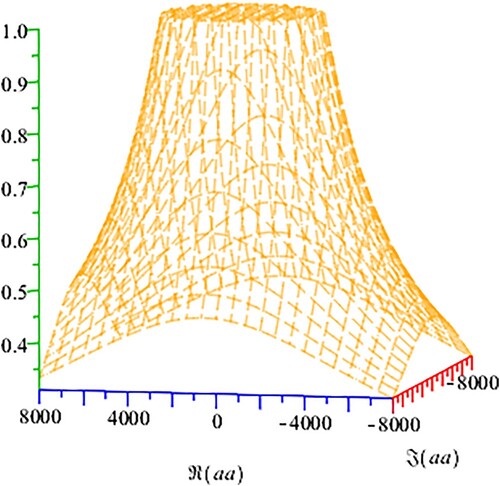
Figure 3. (a–d) depicts the dynamical planes corresponding to the  stable behaviour of iterative method S1 for various values of $\alpha =-2i,10,20,000\pm 20,000i$ respectively.

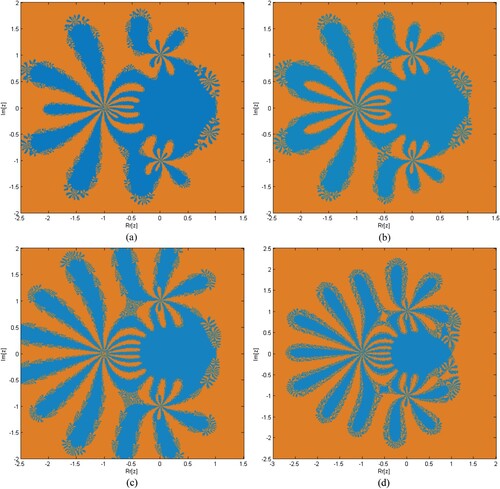
Figure 4. (a,b) depicts the dynamical planes corresponding to the unstable behaviour of iterative method S1 for various values of $\alpha =200\pm 200i$.

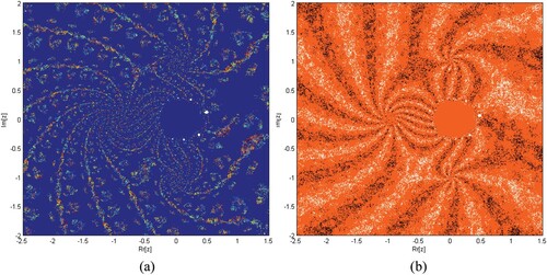
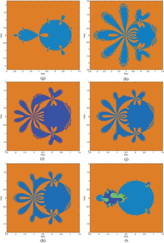
Figure 5. (a-l) depicts the dynamical planes of iterative methods S1–S5, MM1–MM5 for $\alpha =10$, respectively.

The fixed point of for rational map ${\mathrm{\Im }}_{M_1}\left(z,\alpha \right)$ are $z=1$, $z=0$ and $z=\mathrm{\infty }$. For the stability of fixed point of iterative maps ${\mathrm{\Im }}_{M_1}\left(z,\alpha \right),$ we compute ${\mathrm{\Im }}_{M_1}^{\mathrm{\prime }}\left(z,\alpha \right)$.

The fixed points $z=0$ and $z=\mathrm{\infty }$ are always super attractive, as seen in (1d) but the stability of other fixed points depends on the value of the parameter $\alpha$, which is present in this case.

For $z=1$, the operator ${\mathrm{\Im }}_{M_1}^{\mathrm{\prime }}\left(z,\alpha \right)$ yields (45) ${\mathrm{\Im }}_{S_1}^{\mathrm{\prime }}\left(z,\alpha \right)=\left|\frac{32768}{9\alpha -5248}\right|.$(45) The stability of the strange fixed point for $z=1$ is illustrated in the next result.

Theorem 2.2:

The character of the strange point $z=1$ is as follows.

1. if $\left|\alpha -{\displaystyle \frac{5248}{9}}\right|<{\displaystyle \frac{13268}{9}},$ then $z=1$ is an attractor and it can be super attractor for $\alpha =1$

2. when $\left|\alpha -{\displaystyle \frac{5248}{9}}\right|={\displaystyle \frac{13268}{9}}$, $z=1$ is a parabolic point.

3. if $\alpha \ne 0$ and $\left|\alpha -{\displaystyle \frac{5248}{9}}\right|>{\displaystyle \frac{13268}{9}},$ then $z=1$ is a repulsive.

Proof:

It is easy to prove (46) ${\mathrm{\Im }}_{S_1}^{\mathrm{\prime }}\left(1,\alpha \right)=\left|\frac{32768}{9\alpha -5248}\right|.$(46) So, (47) $\left|\frac{32,768}{9\alpha -5248}\right|\le 1\text{ is equivalent to }\left|32,768\right|\le \left|9\alpha -5248\right|.$(47)

Let us consider $\alpha =a+ib$ an arbitrary complex number.

Then (48) $\begin{array}{rl}(9a-5248{)}^2+b^2& \ge (32,768{)}^2,\\ a& \le \frac{1}{4}.\end{array}$(48) therefore $\left|{\mathrm{\Im }}_{S_1}^{\mathrm{\prime }}\left(1,\alpha \right)\right|\le 1$ $iff$ $\left|\alpha -\frac{5248}{9}\right|\ge \frac{32768}{9}.$ Finally, if $\alpha$ varies, then $\left|\alpha -\frac{5248}{9}\right|\le \frac{32768}{9}$ then $\left|{\mathrm{\Im }}_{S_1}^{\mathrm{\prime }}\left(1,\alpha \right)\right|\ge 1$ and $z=1$ is a repulsive, except if $\alpha =1,\alpha =\frac{5248}{9}$ for which $z=1$ is not a fixed point $.$

The functions where we examine stability of iterative method S1 are given as (49) ${\mathrm{\Im }}_{S_1}^{\mathrm{\prime }}\left(1,\alpha \right)=min\left\{{\mathrm{\Im }}_{S_1}^{\mathrm{\prime }}\right(1,\alpha ),1\}.$(49) Dynamical Planes: Parametric planes are obtained by taking $\alpha$ over a mesh of $500\times 500$ values in complex plane in $R_e\left(\alpha \right)\times Im\left(\alpha \right)$ . $\in [-4,4],[-4,4].$ Taking ${10}^{-3}$ as a tolerance used as a stopping criterion. If the technique converges to either of the roots (0 and 1), the complex value of the parameter in the complex plane is painted in various colours, and black in all other cases.

Basins of Attraction: To provoke the basins of attraction of iterative schemes S1–S5, MM1–MM5 for determining the roots of the nonlinear equations, we execute the real and imaginary parts of the starting approximations represented as two axes over a mesh of $250\times 250$ in complex plane. Use $\left|x_{i+1}-x_i\right|<{10}^{-3}$ as a stopping criterion and consider maximum 20 iterations. We allow different colours to mark to which root the iterative scheme converges and black in other cases. Colour brightness in basins shows a less number of iterations.

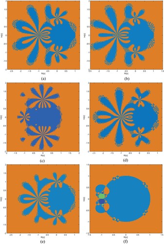
Table 1 clearly shows that the elapsed time of S1–S5 is better than MM1–MM7 for generating the basins of attraction of $f_3\left(x\right),f_{3\ast }\left(x\right),f_5\left(x\right),f_6\left(x\right)$, respectively. Elapsed time and brightness in colour of Figures 6–9(a–f) show dominance in efficiency of our methods S1–S5 as compared to MM1–MM7, respectively.

Figure 6. (a–l) show basins of attraction for methods S1–S5 and MM1–MM7, respectively, for function $f_1\left(x\right)$.

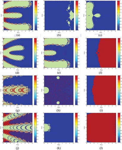
Figure 7. (a–l) show basin of attraction for methods S1–S5 and MM1–MM7, respectively, for function $f_2\left(x\right)$.

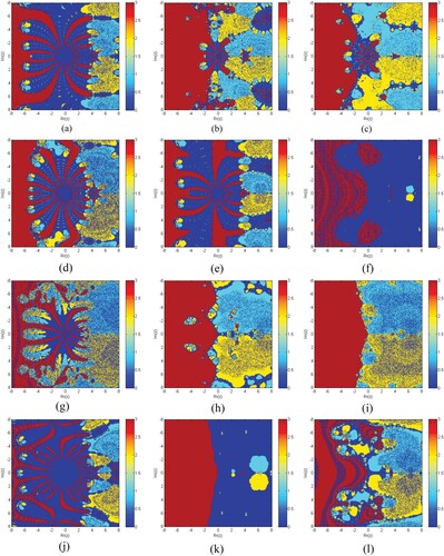
Figure 8. (a–l) show basins of attraction for methods S1–S5 and MM1–MM7, respectively, for function $f_3\left(x\right)$.

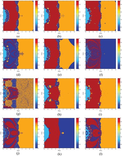
Figure 9. (a–l) show basins of attraction for methods S1–S5 and MM1–MM7, respectively, for function $f_4\left(x\right)$.

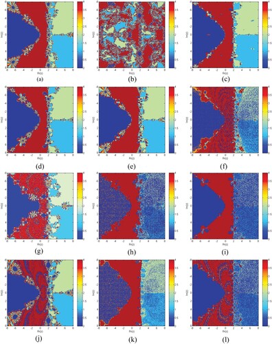
Table 1. Elapsed time in seconds.

Method	S1	S2	S3	S4	S5
$f_3\left(x\right)=-{\displaystyle \frac{9.8}{800}}{x}^2-0.4x+10+{\displaystyle \frac{400}{19.6}}$	0.0714	0.0192	0.03231	0.0714	0.0153
$f_{3\ast }\left(x\right)=e^{x^2}-\log \left(x\right)$	0.0184	0.0177	0.03191	0.0124	0.0191
$f_5\left(x\right)=x^4+4x^3-24x^2+16x+16$	3.1714	4.3152	5.73231	3.2714	2.3152
$f_6\left(x\right)=x^4-7.79075x^3+14.7445x^2+2.511x-1.674$	3.9124	4.0193	3.83191	2.5124	3.0153
MM1	MM2	MM3	MM4	MM5	MM6	MM7
3.1422	4.3231	7.1293	8.1422	4.3231	0.0714	0.0152
1.2382	1.4319	2.1609	3.2482	3.4719	1.1124	4.2193
4.1422	5.3231	5.1293	5.1422	4.3231	5.4714	5.9152
7.2382	7.4819	6.1659	5.2382	5.4319	8.1124	5.0193

3 Numerical outcomes

Some numerical examples [5,9,10,18,25–32] are being used to test the efficiency of our three-step eight-order single root finding methods S1–S5 compared to MM1–MM7. All computations are performed in Maple 18 with 2500 significant digits and the following termination criteria: $e_i=\left|f\left(x_i\right)\right|<\in ,\left(ii\right)e_i=\left|x_i-\zeta \right|<\in ,$where $e_i$ represents the absolute error of function values in $\left(i\right)$ and norm-2 in $\left(ii\right)$ [8]. We take $\in ={10}^{-200}$ for single root finding method. Numerical tests examples are provided in Tables 2–7. In all tables, $\rho$ represents computational order of convergence [14] and CPU represents computational time in seconds.

3.1 Real-world application

In this section, we discuss some real-world applications whose solutions are approximated by our newly constructed methods S1–S5.

Table 2. Numerical comparison of S1–S5 and MM1–MM7.

Method	$\left|x_3-\zeta \right|$	$\left|f\left(x_3\right)\right|$	CPU	$\rho$
$f_1\left(x\right)=c-{\displaystyle \frac{\pi {\left({\displaystyle \frac{h}{\cos \left(x\right)}}\right)}^{2}F}{0.5\pi D^2\left(1+\sin \left(x\right)-0.5\cos \left(x\right)\right)}}$
S1	0.3e−157	3.1e−322	0.0130	7.9
S2	4.1e−150	0.8e−319	0.0124	8.0
S3	3.3e−160	0.4e−320	0.0113	8.0
S4	6.4e−153	9.8e−325	0.0182	8.0
S5	0.5e−161	2.8e−331	0.0171	7.9
MM1	9.3e−118	0.3e−144	0.0274	7.9
MM2	1.8e−120	6.7e−140	0.0361	8.0
MM3	8.3e−137	7.2e−145	0.0252	8.01
MM4	7.1e−140	9.9e−150	0.0328	7.89
MM5	4.6e−125	9.2e−180	0.0179	8.9
MM6	6.2e−117	8.3e−175	0.0327	8.1
MM7	5.5e−116	3.3e−140	0.0251	8.0

Table 3. Numerical comparison of S1–S5 and MM1–MM7.

Method	$\left|x_3-\zeta \right|$	$\left|f\left(x_3\right)\right|$	CPU	$\rho$
$f_2\left(x\right)=v\left(t\right)-\sqrt{2gx}\times \tanh \left({\displaystyle \frac{t}{2l}}\sqrt{2gx}\right)$
S1	7.3e−182	9.1e−224	0.0134	8.0
S2	3.5e−185	5.0e−220	0.0151	8.0
S3	0.3e−190	0.4e−235	0.0140	8.0
S4	0.4e−180	0.8e−231	0.0123	7.0
S5	6.5e−181	8.1e−219	0.0112	6.9
MM1	8.3e−130	3.7e−170	0.0274	7.9
MM2	9.3e−133	2.6e−170	0.0365	8.0
MM3	4.9e−135	4.2e−171	0.0255	8.0
MM4	8.1e−140	5.9e−165	0.0267	8.0
MM5	0.4e−141	9.2e−117	0.0196	7.9
MM6	2.2e−137	8.3e−155	0.0227	7.8
MM7	3.5e−138	1.2e−173	0.0238	8.1

Table 4. Numerical comparison of S1–S5 and MM1–MM7.

Method	$\left|x_3-\zeta \right|$	$\left|f\left(x_3\right)\right|$	CPU	$\rho$
$f_3\left(x\right)=-{\displaystyle \frac{9.8}{800}}{x}^2-0.4x+10+{\displaystyle \frac{400}{19.6}}$
S1	5.3e−61	2.1e−495	0.0151	7.9
S2	4.5e−71	5.8e−577	0.0141	8.0
S3	6.3e−73	4.4e−592	0.0153	8.0
S4	2.4e−78	6.8e−636	0.0164	8.2
S5	2.5e−64	2.1e−522	0.0152	8.1
MM1	5.3e−16	3.5e−67	0.0474	7.0
MM2	1.3e−37	2.7e−231	0.0169	8.0
MM3	4.3e−39	2.2e−202	0.0158	8.0
MM4	4.1e−42	4.9e−259	0.0169	6.7
MM5	4.4e−31	1.2e−417	0.0164	7.9
MM6	1.2e−17	6.3e−474	0.0166	7.8
MM7	1.5e−66	3.2e−540	0.0155	7.9

Table 5. Numerical comparison of S1–S5 and MM1–MM7.

Method	$\left|x_3-\zeta \right|$	$\left|f\left(x_3\right)\right|$	CPU	$\rho$
$f_4\left(x\right)=-100\ast {10}^{-9}{x}^3+9.3100\ast x^2-18.6200\ast x+9.3100$
S1	4.7e−130	1.5e−722	0.0213	8.1
S2	5.0e−135	2.1e−735	0.0252	8.0
S3	2.1e−136	1.2e−711	0.0251	7.9
S4	1.2e−137	4.6e−773	0.0242	7.9
S5	2.9e−138	1.5e−647	0.0262	8.0
MM1	1.6e−88	3.0e−334	0.0333	7.9
MM2	4.9e−81	2.5e−335	0.0315	7.7
MM3	9.0e−75	1.4e−216	0.0264	6.9
MM4	1.0e−50	5.0e−154	0.0376	7.5
MM5	7.1e−49	1.7e−187	0.0284	7.9
MM6	3.4e−55	3.1e−197	0.0375	7.7
MM7	3.7e−96	6.8e−563	0.0367	8.1

Table 6. Numerical comparison of S1–S5 and MM1–MM7.

Method	$\left|x_3-\zeta \right|$	$\left|f\left(x_3\right)\right|$	CPU	$\rho$
$f_5\left(x\right)=x^4+4x^3-24x^2+16x+16$
S1	4.7e−91	1.5e−721	0.0151	7.9
S2	5.0e−101	2.1e−802	0.0152	8.0
S3	2.1e−103	1.2e−821	0.0153	8.1
S4	1.2e−109	4.6e−873	0.0151	7.9
S5	2.9e−94	1.5e−747	0.0163	8.0
MM1	1.6e−23	3.0e−90	0.0314	7.9
MM2	4.9 −35	2.5 e−325	0.0165	8.0
MM3	9.0e−30	1.4e−116	0.0165	7.9
MM4	1.0e−59	5.0e−354	0.0167	8.0
MM5	7.1e−49	1.7e−287	0.0168	7.9
MM6	3.4e−25	3.1e−97	0.0319	7.7
MM7	3.7e−96	6.8e−763	0.0166	7.8

Table 7. Numerical comparison of S1–S5 and MM1–MM7.

Method	$\left|x_3-\zeta \right|$	$\left|f\left(x_3\right)\right|$	CPU	$\rho$
$f_6\left(x\right)=x^4-7.79075x^3+14.7445x^2+2.511x-1.674$
S1	4.8e−16	1.3e−120	0.0162	8.0
S2	7.4e−29	9.4e−224	0.0161	7.9
S3	5.7 e−26	1.5e−200	0.0160	8.0
S4	3.5 e−29	1.6e−226	0.0161	8.1
S5	4.0e−20	5.5e−154	0.0153	7.9
MM1	2.4e−6	1.5e−21	0.0314	7.9
MM2	1.0e−22	8.7e−131	0.0165	8.0
MM3	3.9 e−16	7.5e−162	0.0167	7.0
MM4	1.1 e−19	6.4e−113	0.0158	7.9
MM5	5.1e−5	5.8e−124	0.0163	7.5
MM6	8.4e−8	1.4e−127	0.0164	7.5
MM7	3.3e−25	2.6e−194	0.0158	8.0

3.1.1 Solar energy system: a mechanical engineering problem

In studies of solar energy collection by focusing a field of plane mirrors on a central collector, one researcher obtained the following equation for geometrical concentration factor c: (50) $\begin{array}{rl}c& =\frac{\pi {\left(\frac{h}{\cos \left(x\right)}\right)}^{2}F}{0.5\pi D^2\left(1+\sin \left(x\right)-0.5\cos \left(x\right)\right)},\end{array}$(50) (51) $\begin{array}{rl}{f}_1\left(x\right)& =c-\frac{\pi {\left(\frac{h}{\cos \left(x\right)}\right)}^{2}F}{0.5\pi D^2\left(1+\sin \left(x\right)-0.5\cos \left(x\right)\right)},\end{array}$(51) where $x$ is the rim angle of the field. F is the fraction coverage of the field with mirrors. D is the diameter of the collector and h is the height of the collector. To find rim angle $x$ i.e. solution of (51), we choose h = 300, c = 1200, F = 0.8, and D = 14 and choose $x_0=0.9,$ where $\zeta =0.8570854843$.

The corresponding results for $f_1\left(x\right)$ are clearly shown in Table 2. The theoretical order of convergence matches the computational order of convergence. On the same number of iterations, the computation residual error of our iterative schemes S1–S5 are better than MM1–MM5.

3.1.2 Water discharge problem

Water is discharged from a reservoir through a long pipe. By neglecting the change in the level of the reservoir, the transient velocity v(t) of the water flowing from the pipe at time t is given by (52) $\begin{array}{rl}v\left(t\right)& =\sqrt{2gx}\times \tanh \left(\frac{t}{2l}\sqrt{2gx}\right),\end{array}$(52) (53) $\begin{array}{rl}{f_2}_{}\left(x\right)& =v\left(t\right)-\sqrt{2gx}\times \tanh \left(\frac{t}{2l}\sqrt{2gx}\right),\end{array}$(53) where h is the height of the fluid in the reservoir, $l$ is the length of the pipe, g = 9.81 m/s${}^2$ is gravity. Finding the value of h necessary to achieve a velocity of v = 4 m/s at time t = 4 sec, when $l$ = 5 m. Using S1–S5, MM1–MM7 numerical iterative methods for calculating the exact root of (53), we start with $x0=1$ and obtain the following results.

The corresponding results for $f_2\left(x\right)$ are clearly shown in Table 3. The theoretical order of convergence matches the computational order of convergence. On the same number of iterations, the computation residual error of our iterative schemes S1–S5 are better than MM1–MM5.

3.1.3 Projectile motion

Consider a projectile [17,18,30] which is projected from a tower of height $h>0$ onto a hill with initial speed v with angle $\theta .$ Define an impact function $\omega \left(x\right)$ which depends on horizontal distance x. The path function of projectile is defined as (54) $P\left(x\right)=h+x\tan \theta -\frac{g{x}^2}{2v^2}{\sec }^2\theta .$(54) When the projectile hits the hill there exist a value of x for which $P\left(x\right)=\omega \left(x\right)$. We have to find such a value of $\theta$ which maximizes $x,$ therefore differentiating (54) with respect to $\theta$ i.e. (55) ${\omega }^{\mathrm{\prime }}\left(x\right)\frac{dx}{d\theta }=x{\sec }^2\theta +\frac{dx}{d\theta }-\frac{g}{v^2}(x^2{\sec }^2\theta \tan \theta +x\frac{dx}{d\theta }{\sec }^2\theta ),$(55) putting $\frac{dx}{d\theta }=0,$ we have: (56) $\begin{array}{rl}x& =\frac{v^2}{g}\cot \theta ,\end{array}$(56) (57) $\begin{array}{rl}\theta & ={\tan }^{-1}\left(\frac{v^2}{gx}\right).\end{array}$(57) Taking enveloping parabola $\omega =\tan \theta$ [27], we have: (58) $y=P\left(x\right)=h+x\omega -\frac{g{x}^2}{2v^2}(1+{\omega }^2).$(58) Differentiating (58) and setting $y^{\mathrm{\prime }}=0,$ we have: (59) $\begin{array}{rl}{y}^{\mathrm{\prime }}& =x-\frac{x{g}^2}{v^2}\left(\omega \right),\end{array}$(59) (60) $\begin{array}{rl}\omega & =\frac{v^2}{gx}.\end{array}$(60) Thus, our enveloping parabola becomes: (61) $y=\rho \left(x\right)=h+\frac{v^2}{2g}-\frac{g{x}^2}{2v^2}.$(61) For the solution of the parabola first we find x by taking $\omega \left(x\right)=0.4x$ and $h=10,v=20,g=9.8,$ in (47), we can write: $f\left(x\right)=\rho \left(x\right)-\omega \left(x\right)=h+\frac{v^2}{2g}-\frac{g{x}^2}{2v^2}-0.4x,$ (62) $f_3\left(x\right)=-\frac{9.8}{800}{x}^2-0.4x+10+\frac{400}{19.6}=-0.01225x^2-0.4x+30.40816327,$(62) and (63) ${\theta }_m={\tan }^{-1}\left(\frac{v^2}{g{x}_m}\right)={48.5}^o.$(63) The exact roots of (62) are ${\zeta }_1=36.102970117,{\zeta }_2=-\mathrm{68.756.}$

The initial estimate for $f_3\left(x\right)$ is taken as $x_0=30$:

The corresponding results for $f_3\left(x\right)$ are clearly shown in Table 4. The theoretical order of convergence matches the computational order of convergence. On the same number of iterations, the computation residual errors of our iterative schemes S1–S5 are better than MM1–MM5.

3.1.4 Fluid permeability in bio gels:

Specific hydraulic permeability [34] relates the pressure gradient to fluid velocity in a porous medium (agarose gel or extracellular fibre matrix) and is shown in the following non-linear polynomial equations: (64) $\mathbf{k}=\frac{{R_e}^2{x}^3}{20{(1-x)}^2},$(64) or (65) $R_e{x}^3-20\mathbf{k}(1-x{)}^2=0,$(65) where $\mathbf{k}$ is specific hydraulic permeability, $R_e$ radius of the fibre, and $x$ is the porosity [35]. Using $\mathbf{k}=0.4655$ and $R_e=100\ast {10}^{-9},$ we have: (66) $f_4\left(x\right)=-100\ast {10}^{-9}{x}^3+9.3100\ast x^2-18.6200\ast x+\mathrm{9.3100.}$(66) The exact roots of (66) are ${\zeta }_1=0.9999999997,{\zeta }_2=1.000000000,{\zeta }_3=9.31\ast {10}^{18}.$

We choose $\stackrel{\left(0\right)}{x}=9.3\ast {10}^{17}$ as an estimate for determination of roots (66).

The corresponding results for $f_4\left(x\right)$ are clearly shown in Table 5. The theoretical order of convergence matches the computational order of convergence. On the same number of iterations, the computation residual error of our iterative schemes S1–S5 are better than MM1–MM5.

3.1.5 Beam designing model [29]

Consider a problem of beam positioning [25,26], resulting in a nonlinear function given as (67) $f_5\left(x\right)=x^4+4x^3-24x^2+16x+16=(x-2{)}^2(x^2+8x+4).$(67) The exact roots of (67) are ${\zeta }_{1,2}=2,{\zeta }_3=-4-2\sqrt{3},{\zeta }_3=2,{\zeta }_4=-4+2\sqrt{3}.$

The initial estimates for $f_5\left(x\right)$ are taken as $x_0=-0.5$ our required exact root is 2.

The corresponding results for $f_5\left(x\right)$ are clearly shown in Table 6. The theoretical order of convergence matches the computational order of convergence. On the same number of iterations, the computation residual error of our iterative schemes S1–S5 are better than MM1–MM5.

3.1.6 Fractional conversion [28,29]

The following expression [31,32] describes the fractional conversion of nitrogen, hydrogen feed at 250 atm. and 227 K. (68) $f_6\left(x\right)=x^4-7.79075x^3+14.7445x^2+2.511x-\mathrm{1.674.}$(68) The exact roots of (68) are ${\zeta }_1=3.9485+0.3161i,{\zeta }_2=3.9485-0.3161i,{\zeta }_3=-0.3841,{\zeta }_4=\mathrm{0.2778.}$

The initial estimate for $f_6\left(x\right)$ is taken as $x_0=0.1$ and our desired exact roots is $0.2778$.

The corresponding results for $f_6\left(x\right)$ are clearly shown in Table 7. The theoretical order of convergence matches the computational order of convergence. On the same number of iterations, the computation residual error of our iterative schemes S1–S5 are better than MM1–MM5.

4 Conclusion

A new family of optimal three-point eighth-order numerical iterative algorithms for approximating a simple root of a given nonlinear equation is developed using the weight function technique. The software CAS-Maple has been used to prove that the optimal technique is convergent with convergence order equals eight. The methods require only four function evaluations every iteration, resulting in an optimal order eight method. As a result, the Kung and Traub conjecture holds true for the new methods. The proposed schemes are tested against various existing schemes, demonstrating the superiority of the proposed methods. Six  engineering application problems are solved, including projectile motion, beam designing model, and fractional conversion, with the new approaches excelling the other methods. Further research has been done on the complex plane for such methods to expose their basins of attraction for solving complex polynomials by presenting the fractal graphs that correlate to them. The numerical results of the proposed methods, as well as the elapsed time for their fractal graphs in Table 1, indicate that the novel methods are a feasible alternative for solving scalar nonlinear equations. Tables 1–7 show the numerical results. On the third iteration, Tables 2–7 clearly show that the residual error, CPU time, and local computational order of convergence of newly proposed methods S1–S5 are significantly superior to existing methods MM1–MM7.

Disclosure statement

No potential conflict of interest was reported by the author(s).

References

- Consnard M, Fraigniaud P. Finding the roots of a polynomial on an MIMD multicomputer. Parallel Comput. 1990;15(1):75–85.
- Agarwal P, Filali D, Akram M, et al. Convergence analysis of a three-step iterative algorithm for generalized set-valued mixed-ordered variational inclusion problem. Symmetry (Basel). 2021;13(3):444.
- Sunarto A, Agarwal P, Sulaiman J, et al. Iterative method for solving one-dimensional fractional mathematical physics model via quarter-sweep and PAOR. Adv Differ Equ. 2021;1:147.
- Attary M, Agarwal P. On developing an optimal Jarratt-like class for solving nonlinear equations. Ital J Pure Appl Math. 2020;43:523–530.
- Sendov B, Andereev A, Kjurkchiev N. Numerical solutions of polynomial equations. New York: Elsevier science; 1994.
- Wang X, Liu L. Modified Ostrowski’s method with eight -order convergence and high efficiency index. Appl Math Lett. 2010;23:549–554.
- Li TF, Li DS, Xu ZD, et al. New iterative methods for non-linear equations. Appl Math Comput. 2008;2:755–759.
- Kumar S, Kumar D, Sharma JR, et al. An optimal fourth order derivative-free numerical algorithm for multiple roots. Symmetry (Basel). 2020;12(6):1038.
- Mir NA, Muneer R, Jabeen I. Some families of two-step simultaneous methods for determining zeros of non-linear equations. ISRN Appl Math. 2011;2011:1–11.
- Farmer MR. Computing the zeros of polynomials using the divide and conquer approach. [dissertation]. Ph.D Thesis. Department of Computer Science and Information Systems, Birkbeck: University of London; 2014.
- Bi W, Ren H, Wu Q. Three-step iterative methods with eighth-order convergence for solving nonlinear equations. J Comput Appl Math. 2009;225:105–112.
- Chun C, Ham YM. Some sixth-order variants of Ostrowski root-finding methods. Appl Math Comput. 2007;193:389–394.
- Wang X, Liu L. Two new families of sixth-order methods for solving non-linear equations. Appl Math Comput. 2009;213(1):73–78.
- Jay LO. A note on Q-order of convergence. Bit Numer Math. 2001;41:422–429.
- Babajee DKR, Cordero A, Soleymani F, et al. On improved three-step schemes with high efficiency index and their dynamics. Numer Algor. 2014;65:153–169.
- Cordero A, Fardi M, Ghasemi M, et al. Accelerated iterative methods for finding solutions of nonlinear equations and their dynamical behavior. Calcolo. 2014;51:17–30.
- Sharma JR, Sharma R. A new family of modified Ostrowski’s methods with accelerated eighth order convergence. Numer Algor. 2010;54:445–458.
- Liu L, Wang X. Eighth-order methods with high efficiency index for solving nonlinear equations. Appl Math Comput. 2010;215:3449–3454.
- Wang X, Liu L. New eighth-order iterative methods for solving nonlinear equations. J Comput Appl Math. 2010;234:1611–1620.
- Kung HT, Traub JF. Optimal order of one-point and multipoint iteration. J Assoc Comput Mach. 1974;21(643):651.
- Shacham M. An improved memory method for the solution of a nonlinear equation. Chem Eng Sci. 1989;44:1495–1501.
- Balaji GV, Seader JD. Application of interval Newton’s method to chemical engineering problems. Reliab Comput. 1995;1:215–223.
- Babajee DKR, Madhu K. Comparing two techniques for developing higher order two-point iterative methods for solving quadratic equations. SeMA J. 2018; 76(2):1–22.
- Kantrowitz R, Neumann MM. Some real analysis behind optimization of projectile motion. Mediterr J Math. 2014;11:1081–1097.
- Keshet EL. Differential calculus for the life sciences. Vancouver, BC: University of British Columbia; 2017.
- Zachary JL. Introduction to scientific programming: computational problem solving using Maple and C. New York (NY): Springer; 2012.
- Henelsmith N. Finding the optimal launch angle. Walla Walla (WA): Whitman College; 2016.
- Chicharro FI, Cordero A, Garrido N, et al. Stability and applicability of iterative methods with memory. J Math Chem. 2019;57(5):1282–1300.
- Zafar F, Cordero A, Torregrosa JR. An efficient family of optimal eighth-order multiple root finders. Mathematics. 2018;6:310.
- Tao Y, Madhu K. Optimal fourth, eighth and sixteenth order methods by using divided difference techniques and their basins of attraction and its application. Mathematics. 2019;7:322.
- Argyros IK, Magreñán AA, Orcos L. Local convergence and a chemical application of derivative free root finding methods with one parameter based on interpolation. J Math Chem. 2016;54:1404–1416.
- Fournier RL. Basic transport phenomena in biomedical engineering. New York (NY): Taylor & Franics; 2007.
- Saltzman WM. Drug delivery: engineering principal for drug therapy. New York (NY): Oxford University Press; 2001.