Contaminant transport analysis under non-linear sorption in a heterogeneous groundwater system

ABSTRACT

In this study, a one-dimensional non-linear advection–dispersion equation subject to spatial–temporal dependent advection and dispersion coefficients is solved for a heterogeneous groundwater system. The non-linearity of the governing equation is based on the Freundlich and Langmuir sorption isotherms. The groundwater flow is considered to vary exponentially with time. Also, a generalized theory of the dispersion coefficient is used for extensive study of the model problem. The approximate solutions of the model problem are obtained in a semi-infinite and finite heterogeneous media by employing the Crank–Nicolson scheme. The exact solutions are obtained in both domains by the Laplace transform technique subject to linear sorption isotherm and non-transient flow conditions. Further, various graphical solutions are obtained using MATLAB scripts to examine the contaminant transport behaviour. For quantitative evaluation of the proposed model, a root mean square (RMS) error is computed. Overall, the results show that RMS error of the approximate solutions with respect to the exact solutions is within acceptable limits (less than 5%) for different combinations of discretization parameters. The robustness of the proposed model suggests its better suitability for modelling groundwater transport phenomena under the consideration of a non-linear sorption isotherm.

KEYWORDS:

• Advection
• dispersion
• groundwater contamination
• heterogeneous medium
• non-linear sorption
• transient flow

2010 MSC CODES:

• 35K57
• 35K20
• 76M20
• 76S20

Nomenclature

$c\text{[}\text{M}{\text{L}}^{-3}\text{]}$	=	Liquid phase contaminant concentration
$R\text{[}-\text{]}$	=	Retardation factor
$S\text{[}\text{M}{\text{M}}^{-1}\text{]}$	=	Solid phase contaminant concentration
$\rho \text{[}\text{M}{\text{L}}^{-3}\text{]}$	=	Density
$\varphi \text{[}-\text{]}$	=	Porosity
$\eta \text{[}{\text{T}}^{-1}\text{]}$	=	First-order decay rate coefficient
$\delta \text{[}\text{M}{\text{L}}^{-3}{\text{T}}^{-1}\text{]}$	=	Zero-order production rate
$u_1\text{[}\text{L}{\text{T}}^{-1}\text{]}$	=	Advection coefficient
$D_1\text{[}{\text{L}}^2{\text{T}}^{-1}\text{]}$	=	Dispersion coefficient
$x\text{[}\text{L}\text{]}$	=	Distance variable
$t\text{[}\text{T}\text{]}$	=	Time variable
$k_d\text{[}{\text{M}}^{-1}{\text{L}}^{-3}\text{]}$	=	Sorption coefficient
$k_l\text{[}\text{M}{\text{M}}^{-1}\text{]}$	=	Maximum sorption capacity
$u_0\text{[}\text{L}{\text{T}}^{-1}\text{]}$	=	Average soil water flow velocity
$D_0\text{[}{\text{L}}^2{\text{T}}^{-1}\text{]}$	=	Constant dispersion coefficient
$m\text{[}{\text{T}}^{-1}\text{]}$	=	Flow resistant coefficient
$b\text{[}{\text{L}}^{-1}\text{]}$	=	Heterogeneity parameter of the porous medium
$c_0\text{[}\text{M}{\text{L}}^{-3}\text{]}$	=	Initial constant solute concentration
$c_1\text{[}\text{M}{\text{L}}^{-3}\text{]}$	=	Input concentration

Introduction

Groundwater, which typically refers to the water occupied in the void spaces of the Earth’s sub-surface soil strata, may be contaminated by various anthropogenic activities or natural phenomena. The analysis of contaminant or solute transport in a groundwater system has become indispensable to deal with groundwater contamination. The solute transport in a porous medium is mathematically modelled as the advection–dispersion equation (ADE). The dissolved solute constituents in a saturated medium may be partially adsorbed by soil particles known as solid-phase concentration. In addition to the sorption, there may be decay or production of the solute in the medium representing as source/sink term in the governing ADE [1].

Extensive studies of the solute fate and transport in porous media have been reported in the past using various analytical approaches. van Genuchten [2] presented several analytical results derived by the Laplace transform technique (LTT) of a one-dimensional (1D) ADE under the consideration of linear equilibrium adsorption, first-order decay (FOD), and zero-order production (ZOP) subject to various initial and boundary conditions to examine the fate and transport of chemical in semi-infinite porous media. Yates [3] applied LTT to solve a 1D solute transport equation in inhomogeneous transport media subject to asymptotic space varying dispersion relationship and constant boundary conditions. The exact solution was obtained in terms of hypergeometric function. Serrano [4] presented the approximate analytical solutions of 1D ADEs in an infinite domain to analyze the contaminant plume transport behaviour for linear and non-linear sorption. The analytical solutions were obtained in series form for the reversible and irreversible kinetic sorption models. The authors concluded that, for a more realistic treatment of the contaminant distribution, the non-linear sorption model is more suited when compared to the linear sorption model.

Guerrero and Skaggs [5] produced an exact solution of solute fate and transport in a finite non-uniform transport media. The solution was obtained by transforming a general ADE with space-dependent coefficients, using the integrating factor and generalized integral transform technique (GITT). The general solution was developed by first solving the governing equation in a steady-state regime, followed by transformation of a non-self-adjoint equation using an integrating factor, and finally obtained the required solution using the GITT. Kumar et al. [6] derived an exact solution of a 1D solute transport along with the transient longitudinal flow in an inhomogeneous semi-infinite extent medium. The impact of inhomogeneity and transient flow on solute transport was examined. Moreover, van Genuchten et al. [7] studied the 1D solute transport with FOD and ZOP in the equilibrium state. The exact solution was obtained by applying the LTT. Guerrero et al. [8] used the Duhamel theorem, which is typically applied to solve diffusion problems, for obtaining the solution of a 1D solute transport in porous formations subject to temporally dependent boundary conditions. They developed and compared the solutions for standard cases, such as instantaneous and finite pulse applications, whose exact solutions were known. Wadi et al. [9] obtained the analytical solution of a 1D pollutant transport in a semi-infinite homogeneous river by the LTT. Hayek [10] studied the analytical model for contaminant fate and transport in an infinite transport formation subject to temporally varying parameters. The Fourier transform method was used to find the exact solution. The importance of the given model was for analyzing the contaminant transport in deformable formations where both the dispersion and advection coefficients vary with time. Purkayastha and Kumar [11] also discussed the analytical solution of a 1D ADE subject to temporally varying contaminant conditions. The diffusivity and advection terms were defined as varying spatially. The Eigenfunction expansion technique was employed to obtain the solution of the transformed governing equation. Molati and Murakawa [12] derived the analytical solution of a non-linear contaminant transport equation by applying the Lie symmetry method. Few studies in the literature [13–17] also suggest the use of the similarity transform method, which is used to reduce the partial differential equation to the system of an ordinary differential equation, for obtaining model solutions of few generic transports.

It is apparent from the literature that the analytical approaches are generally complicated for solving the modelling problems for a realistic environment which typically includes several parameters. However, following the advancements in the computational infrastructure, numerical approaches are generally preferred in place of the analytical approaches to deal with complex type model problems. Using numerical techniques (such as finite element method (FEM), finite difference method (FDM), etc.), a complex solute transport model problem can be derived approximately with reasonable accuracy subject to arbitrary initial and complicated boundary conditions. Bosma and van Der Zee [18] presented approximate solutions for the solute transport phenomena for the transportation of cadmium through the soil under non-linear adsorption in steady-state flow. A large number of different combinations of the chemically heterogeneous soil columns are generated using a random generator. It is observed that, for a single realization, the non-linear nature of the adsorption phenomenon may be significant. In contrast, for an ensemble column, the effect may be diminished, and variations are relatively smooth. Further, Dehghan [19] solved the 1D solute transport equation for a finite length aquifer using several kinds of explicit and implicit FDMs and found the explicit FDM as an efficient method to deal with the higher dimensional transport equations compared to the implicit FDM. Fares and Giacobbe [20] studied the unsteady migration of non-conservative and conservative solutes in soil systems and used the Crank–Nicolson (CN) method for obtaining the numerical solutions of the formulated ADE. Further, Maraqa [21] numerically explored the linear sorption effect on the retardation induced by non-linear sorption of solute in transport media. The experimental results revealed that the retardation depends on input source concentration, the source injection time period, and the fluid flow velocity in the porous medium except for the length scale. Savovic and Djordjevich [22] presented the numerical solutions of horizontal solute transport in a heterogeneous medium using explicit FDM. The solutions were obtained for a time-varying solute spread in a steady flow field through the homogenous formation; solute spread along with steady flow through the heterogeneous formation, and along with the transient flow through the heterogeneous formation. Again, Savovic and Djordjevich [23] numerically solved the 1D ADE subject to pulse-type source injection in a porous medium by explicit FDM. The explicit FDM was found as a suitable method for solving the model equation subject to arbitrary solution conditions. Gharehbaghi [24] solved the 1D temporally dependent contaminant transport equation with space varying coefficients in a heterogeneous semi-infinite transport domain. The governing equation was solved by a differential quadrature method using explicit as well as implicit schemes and found that the implicit method was more accurate and powerful than the explicit method. The approximate solutions were also compared with an existing analytical solution.

Some recent works based on the solute transport under the sorption condition have been reported and dealt with either analytical or numerical approaches. Mojtabi and Deville [25] solved a 1D time-dependent linear ADE subject to Dirichlet homogenous boundary conditions by applying the variable separable method and FEM. The exact solution was compared with the approximate solution for different values of viscosity subject to the constant flow velocity. Gorokhovski and Trofimov [26] studied the solute transport problem under the consideration of sorption isotherms and degradation along the streamlines in porous media. The governing ADE was solved analytically by transforming it into the advection equation. Moranda et al. [27] presented the exact solution of a 1D convection–diffusion equation for reactive solute with sorption and FOD. The LTT was used to solve the governing equation under the consideration of third type time dependent boundary condition. For the transient flow condition, Li et al. [28] studied the solute fate and transport in which the flow varied exponentially. It was observed that a higher exponent led to a faster solute transport process for an exponentially and temporally rising forms of the flow velocity. Time-dependent boundary conditions with two stages point source were considered by Yadav and Roy [29] to solve a 1D ADE under FOD and ZOP in a semi-infinite inhomogeneous porous formation. Das and Singh [30] presented the exact solution of a 1D ADE under linear sorption, FOD, and ZOP in uniform semi-infinite porous media subject to various types of time varying dispersion coefficients. The advection coefficient was expressed as varying exponentially with time. An approximate solution was also derived by explicit FDM to compare with the analytical solution. Singh et al. [31] studied the 1D ADE under the consideration of linear sorption, FOD, and ZOP in a semi-infinite uniform soil formation by the LTT and CN methods. Exact and approximate solutions of the transport equation were derived to analyze the solute dispersion profiles with an intermediate input source in the porous formations. Banaei et al. [32] numerically and experimentally studied the groundwater movement and reactive or non-reactive solute transport in a semi-infinite soil formation. The governing equation was solved by explicit FDM and validated with the existing exact solution as well as experimental results. They concluded that the advection process was the main process to take part in the conservative and non-conservative pollutant transports for the case of high velocity.

The contaminant transport through porous formations based on fieldwork generally requires readymade analytical or numerical solutions to validate the experimental results. Naveen et al. [33] studied the leakage of municipal dump landfill areas to account for the contamination of the surface water as well as groundwater. Although the analytical solution was used to analyze the contaminant transport parameter, they did not validate the experimental results using numerical models, which is critical to generalize the outcomes of such experimental validation. There are numerous studies available in the literature based on analytical approaches. However, investigations of the non-linear governing ADE using the numerical approaches are scarce. To the authors’ best knowledge, there is no such study available so far based on the CN method. Considering these research gaps, we propose a novel numerical scheme for studying a reactive contaminant transport subject to transient groundwater flow, which is solved numerically in the finite and semi-infinite heterogeneous media. The Langmuir and Freundlich sorption isotherms, FOD, and ZOP are considered in the present model to examine their influences on the 1D contaminant fate and transport. For the numerical solution, an unconditionally stable CN scheme is applied to approximate the non-linear 1D ADE and provide better results than the FDM [34–37]. The approximate solutions are graphically illustrated in semi-infinite as well as finite domains with the help of the MATLAB computational environment. The exact solutions of the governing transport equation subject to linear sorption and non-transient flow are also derived to check the accuracy of the approximate solutions.

Mathematical model of contaminant transport in a heterogeneous porous formation

The mathematical model for contaminant transport in a porous formation is derived using the concept based on the mass conservation principle and Fick’s diffusion law. In this study, a liquid phase concentration ($c\left[\text{M}{\text{L}}^{-3}\right]$) as well as a solid phase concentration ($S\left[\text{M}{\text{M}}^{-\text{1}}\right]$) are considered under the contaminant sorption. The mathematical model of the sorbing contaminant transport through the soil formation, having density $\rho \left[\text{M}{\text{L}}^{-3}\right]$ and porosity $\varphi$, subject to the FOD rate coefficient ($\eta \left[{\text{T}}^{-1}\right]$) and ZOP rate ($\delta \left[\text{M}{\text{L}}^{-3}{\text{T}}^{-1}\right]$) is symbolically expressed in the vector form as [38]: (1) $\frac{\mathrm{\partial }c}{\mathrm{\partial }t}+\frac{\rho }{\varphi }\frac{\mathrm{\partial }S}{\mathrm{\partial }t}=\mathrm{\nabla }.\left(D_1\left(x,t\right)\mathrm{\nabla }c\right)-\mathrm{\nabla }.\left(u_1\left(x,t\right)c\right)-\eta c+\delta$(1) where, $x\left[\text{L}\right]$ and $t\left[\text{T}\right]$ represent the distance and time variables respectively, $u_1\left[\text{L}{\text{T}}^{-1}\right]$ is the advection coefficient, and $D_1\left[{\text{L}}^2{\text{T}}^{-1}\right]$ is the dispersion coefficient.

The contaminant transport equation in 1D is expressed as [39]: (2) $\frac{\mathrm{\partial }c}{\mathrm{\partial }t}+\frac{\rho }{\varphi }\frac{\mathrm{\partial }S}{\mathrm{\partial }t}=\frac{\mathrm{\partial }}{\mathrm{\partial }x}\left(D_1(x,t)\frac{\mathrm{\partial }c}{\mathrm{\partial }x}-u_1(x,t)c\right)-\eta c+\delta$(2)

The relationship between the liquid phase contaminant concentration and the solid phase concentration sorbed onto the soil particles under a constant temperature is known as isotherm. When the sorption process occurs very fast in comparison to the flow velocity, the sorption process attains an equilibrium state known as the equilibrium sorption isotherm. The present study is based on the equilibrium state sorption isotherm. The sorption isotherm may be either linear or non-linear type. The linear sorption isotherm is applicable to low solute concentration and absorption. In the linear sorption isotherm, there is no upper limit of the solute sorption onto the soil particles. However, the solute transport represents more realistic for the non-linear sorption model as compared to the linear sorption model [4, 40]. There are two types of non-linear sorption; Freundlich and Langmuir. The Freundlich sorption is defined as $S=k_d{c}^{\omega }$, where $k_d\left[{\text{M}}^{-\omega }{\text{L}}^{3\omega }\right]$ is the sorption coefficient and $\omega$ is the empirically determined non-linearity parameter varying from 0 to 1. The Freundlich sorption isotherm is the most preferable and widely used isotherm so far, but it also does not have an upper limit of the solute sorption onto the soil particles. The Langmuir sorption, which specifies an upper limit of the solute sorption onto the soil particle, is defined as $S=\frac{a{k}_{l}c}{1+ac}$, where $a\left[{\text{M}}^{-\text{1}}{\text{L}}^{\text{3}}\right]$ is Langmuir constant and $k_l$ is the highest sorption capacity [1, 41–43]. Using the relationships of either Freundlich or Langmuir sorption isotherms between $S$ and $c$ in Equation (2) yields: (3) $R\frac{\mathrm{\partial }c}{\mathrm{\partial }t}=\frac{\mathrm{\partial }}{\mathrm{\partial }x}\left(D_1(x,t)\frac{\mathrm{\partial }c}{\mathrm{\partial }x}-u_1(x,t)c\right)-\eta c+\delta$(3) where, $R=\{\begin{array}{c}1+\frac{\rho \omega k_d}{\varphi }{c}^{\omega -1}\text{, for Freundlich sorption isotherm}\\ 1+\frac{\rho a{k}_l}{\varphi {\left(1+ac\right)}^2}\text{, for Langmuir sorption isotherm}\end{array}$ is known as the retardation factor.

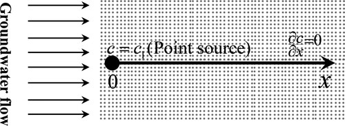
As illustrated by the geometry of the model problem in Figure 1, it is assumed that the groundwater flow follows a horizontal direction with $c_1$ representing the input source. For unsteady groundwater flow in the heterogeneous medium, the generalized theory of seepage velocity over $u_1(x,t)$ is defined as follows [44]: (4) $u_1\left(x,t\right)=u_{0}g\left(mt\right)\left(1+bx\right)$(4) where, $u_0\left[\text{L}{\text{T}}^{-1}\right]$ is the average soil water flow velocity, $m\left[{\text{T}}^{-1}\right]$ is the flow resistant coefficient, and $b\left[{\text{L}}^{-1}\right]$ represents the heterogeneity parameter of the porous medium.

Figure 1. Geometry of the proposed mathematical model.

Again, the generalized theory of dispersion is defined for $D_1\left(x,t\right)$ as follows [44]: (5) $D_1\left(x,t\right)=D_0{g}^{\sigma }\left(mt\right)(1+bx{)}^{\sigma }$(5) where, $D_0\left[{\text{L}}^2{\text{T}}^{-1}\right]$ is a constant dispersion coefficient and the power $\sigma$ is a real number varies from 1 to 2 [45].

Using Equations (4) and (5) in Equation (3), we get (6) $\begin{array}{rl}R\frac{\mathrm{\partial }c}{\mathrm{\partial }t}& =D_0{g}^{\sigma }\left(mt\right)(1+bx{)}^{\sigma }\frac{{\mathrm{\partial }}^{2}c}{\mathrm{\partial }{x}^2}-\left\{u_{0}g\left(mt\right)\left(1+bx\right)-\sigma b{D}_0{g}^{\sigma }\left(mt\right){\left(1+bx\right)}^{\sigma -1}\right\}\frac{\mathrm{\partial }c}{\mathrm{\partial }x}\\ & -\left\{b{u}_{0}g\left(mt\right)+\eta \right\}c+\delta \end{array}$(6)

Initially, the groundwater is considered contaminated uniformly with a constant solute concentration $c_0\left[\text{M}{\text{L}}^{-3}\right]$. The input contaminant $c_1\left[\text{M}{\text{L}}^{-3}\right]$ is assigned at the inlet boundary of the semi-infinite domain. At the extreme point of the domain, Neumann condition is assigned. Thus, the proposed concentration conditions are symbolically expressed as follows: (7) $\begin{array}{rl}c\left(x,t\right)& =c_0;x\ge 0,t=0\end{array}$(7) (8) $\begin{array}{rl}c\left(x,t\right)& =c_1;x=0,t>0\end{array}$(8) (9) $\begin{array}{rl}\underset{x\to \mathrm{\infty }}{lim}\frac{\mathrm{\partial }c}{\mathrm{\partial }x}& =0;t>0\end{array}$(9)

Numerical simulation of the governing transport equation under non-linear sorption

The analytical or numerical solution of a contaminant transport equation is generally used to validate the experimental results or may be helpful to mitigate the groundwater contamination problem. The non-linear ADE (Equation 6) can be approximated using the CN method. Before solving the ADE, first, we need to reduce the semi-infinite spatial domain into a finite domain using the following spatial transformation: (10) $X=L-L\exp \left(-x\right)$(10) where, $L$ is a constant finite spatial length.

Equation (6) takes the following form on using the Equation (10) (11) $R\frac{\mathrm{\partial }c}{\mathrm{\partial }t}=D\left(X,t\right)\frac{{\mathrm{\partial }}^{2}c}{\mathrm{\partial }{X}^2}-u\left(X,t\right)\frac{\mathrm{\partial }c}{\mathrm{\partial }X}-{\eta }_{1}c+\delta$(11) where, $\begin{array}{rl}D\left(X,t\right)& =D_0{g}^{\sigma }\left(mt\right){\left(1+b\log \left(\frac{L}{L-X}\right)\right)}^{\sigma }(L-X{)}^2,\\ u\left(X,t\right)& =D_0{g}^{\sigma }\left(mt\right){\left(1+b\log \left(\frac{L}{L-X}\right)\right)}^{\sigma }\left(L-X\right)\\ & +u_{0}g\left(mt\right)\left(1+b\log \left(\frac{L}{L-X}\right)\right)\left(L-X\right)\\ & -\sigma b{D}_0{g}^{\sigma }\left(mt\right){\left(1+b\log \left(\frac{L}{L-X}\right)\right)}^{\sigma -1}\left(L-X\right)\end{array}$and ${\eta }_1=b{u}_{0}g\left(mt\right)+\eta$.

Also, the concentration conditions in Equations (7)–(9) can be written in the finite spatial domain as follows: (12) $\begin{array}{rl}c\left(X,t\right)& =c_0;X\ge 0,t=0\end{array}$(12) (13) $\begin{array}{rl}c\left(X,t\right)& =c_1;X=0,t>0\end{array}$(13) (14) $\begin{array}{rl}\frac{\mathrm{\partial }c}{\mathrm{\partial }X}& =0;X\to L,t>0\end{array}$(14)

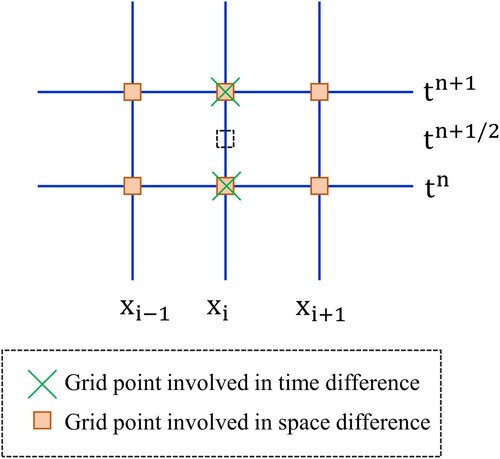
Let the finite spatial and temporal domains be discretized into $P$ and $Q$ sub-intervals, respectively, as illustrated in Figure 2. Again, let each spatial and temporal sub-interval length be represented as $\mathrm{\Delta }X$ and $\mathrm{\Delta }t$, respectively. For the non-linear term involving R as the coefficient in Equation (11), the contaminant concentration at the previous time level (i.e. at the time level $n$) can be used to approximate the retardation factor so that the resultant finite difference approximation would become linearized [43]. Now, applying the CN finite difference scheme in Equation (11) at the grid nodal point $\left(i,n+1/2\right)$, we get (15) $\begin{array}{rl}{R}_i^n\left[\frac{c_i^{n+1}-c_i^n}{\mathrm{\Delta }t}\right]& =\frac{D_i^n}{2}\left[\frac{c_{i+1}^{n+1}-2c_i^{n+1}+c_{i-1}^{n+1}}{\mathrm{\Delta }{X}^2}+\frac{c_{i+1}^n-2c_i^n+c_{i-1}^n}{\mathrm{\Delta }{X}^2}\right]\\ & -\frac{u_i^n}{2}\left[\frac{c_{i+1}^{n+1}-c_{i-1}^{n+1}}{2\mathrm{\Delta }X}+\frac{c_{i+1}^n-c_{i-1}^n}{2\mathrm{\Delta }X}\right]\\ & -\frac{{\eta }_1}{2}\left[c_i^{n+1}+c_i^n\right]+\delta \end{array}$(15) or (16) $A_i^n{c}_{i-1}^{n+1}-E_i^n{c}_i^{n+1}+B_i^n{c}_{i+1}^{n+1}=-A_i^n{c}_{i-1}^n+F_i^n{c}_i^n-B_i^n{c}_{i+1}^n-\delta \mathrm{\Delta }t$(16) where, $i=2,3,4,\dots ,P$, $n=1,2,3,\dots ,Q$, $A_i^n=\frac{D_i^n\left(\mathrm{\Delta }t\right)}{2{\left(\mathrm{\Delta }X\right)}^2}+\frac{u_i^n\left(\mathrm{\Delta }t\right)}{4\left(\mathrm{\Delta }X\right)}$, $B_i^n=\frac{D_i^n\left(\mathrm{\Delta }t\right)}{2{\left(\mathrm{\Delta }X\right)}^2}-\frac{u_i^n\left(\mathrm{\Delta }t\right)}{4\left(\mathrm{\Delta }X\right)}$, $E_i^n=\frac{D_i^n\left(\mathrm{\Delta }t\right)}{{\left(\mathrm{\Delta }X\right)}^2}+\frac{{\eta }_1\left(\mathrm{\Delta }t\right)}{2}+R_i^n$, and $F_i^n=\frac{D_i^n\left(\mathrm{\Delta }t\right)}{{\left(\mathrm{\Delta }X\right)}^2}+\frac{{\eta }_1\left(\mathrm{\Delta }t\right)}{2}-R_i^n$.

Figure 2. Grid discretization by Crank-Nicolson scheme.

Again, the boundary condition (Equation 14) is approximated as follows: (17) $c_{i+1}^n=c_{i-1}^n;i=P+1,n=2,3,\dots ,Q+1$(17)

Applying Equation (17) in Equation (16) yields (18) $\begin{array}{rl}& \left(A_i^n+B_i^n\right)c_{i-1}^{n+1}-E_i^n{c}_i^{n+1}\\ & =-\left(A_i^n+B_i^n\right)c_{i-1}^n+F_i^n{c}_i^n-\delta \mathrm{\Delta }t;i=P+1,n=2,3,\dots ,Q+1\end{array}$(18)

The CN method is used to approximate the governing non-linear transport equation, which is consistent and unconditionally stable. Equations (16) and (18) result in a tridiagonal system of linear equations at each time interval. Consequently, the given system of linear equations is solved by the direct matrix method for a fixed time period using MATLAB script. Similarly, the model problem can also be approximated in the finite spatial domain without applying the transformation (10). The numerical solution is illustrated graphically in semi-infinite and finite media for various hydrological input data in the results and discussion section.

Analytical solution of the governing equation in semi-infinite domain

The governing transport equation is analytically solved under the linear sorption in the steady flow field, and the dispersion is considered directly proportional to the second power of the seepage velocity. Hence, putting $\omega =1$ for linear sorption, $g\left(mt\right)=1$ for steady flow, and $\sigma =2$ in Equation (6), we get (19) $R\frac{\mathrm{\partial }c}{\mathrm{\partial }t}=D_0(1+bx{)}^2\frac{{\mathrm{\partial }}^{2}c}{\mathrm{\partial }{x}^2}-\left\{u_0\left(1+bx\right)-2b{D}_0\left(1+bx\right)\right\}\frac{\mathrm{\partial }c}{\mathrm{\partial }x}-\left(b{u}_0+\eta \right)c+\delta$(19) where, $R=1+\frac{\rho }{\varphi }{k}_d$.

Equation (19) is a linear ADE with variable coefficients. The following transformation in space variable is introduced to change the variable coefficients into constant coefficients: (20) $Y=\frac{1}{b}\log \left(1+bx\right)$(20)

Using Equation (20), Equation (19) is reduced into the following form: (21) $R\frac{\mathrm{\partial }c}{\mathrm{\partial }t}=D_0\frac{{\mathrm{\partial }}^{2}c}{\mathrm{\partial }{Y}^2}-u_2\frac{\mathrm{\partial }c}{\mathrm{\partial }Y}-{\eta }_{2}c+\delta$(21) where, $u_2=u_0-b{D}_0$ and ${\eta }_2=b{u}_0+\eta$.

In this section, the concentration conditions in Equations (7)–(9) are written in the new space variable as follows: (22) $\begin{array}{rl}c\left(Y,t\right)& =c_0;Y\ge 0,t=0\end{array}$(22) (23) $\begin{array}{rl}c\left(Y,t\right)& =c_1;Y=0,t>0\end{array}$(23) (24) $\begin{array}{rl}\frac{\mathrm{\partial }c}{\mathrm{\partial }Y}& =0;Y\to \mathrm{\infty },t>0\end{array}$(24)

To find the exact solution of the Equation (21) by Laplace transform technique, the following concentration transformation is suggested to convert the governing equation into the dispersion equation [25]: (25) $c\left(Y,t\right)=H\left(Y,t\right)\exp \left(\alpha Y+\text{β}t\right)+\frac{\delta }{{\eta }_2}$(25) where, $H\left(Y,t\right)$ represents an arbitrary solute concentration, $\alpha$ and $\text{β}$ are the arbitrary parameters.

From Equations (21) and (25), the parameters $\alpha$ and $\text{β}$ are obtained respectively as follows: (26) $\begin{array}{rl}\alpha & =\frac{u_2}{2D_0}\end{array}$(26) (27) $\begin{array}{rl}\text{β}& =-\frac{1}{R}\left(\frac{u_2^2}{4D_0}+{\eta }_2\right)\end{array}$(27)

Hence, the required concentration transformation is: (28) $c\left(Y,t\right)=H\left(Y,t\right)\exp \left\{\frac{u_2}{2D_0}Y-\frac{1}{R}\left(\frac{u_2^2}{4D_0}+{\eta }_2\right)t\right\}+\frac{\delta }{{\eta }_2}$(28)

Using Equation (28), Equation (21) is reduced into the dispersion equation as follows: (29) $\frac{\mathrm{\partial }H}{\mathrm{\partial }t}=\frac{D_0}{R}\frac{{\mathrm{\partial }}^{2}H}{\mathrm{\partial }{Y}^2}$(29)

Also, the initial and boundary conditions in Equations (22)–(24) take the following forms: (30) $\begin{array}{rl}H\left(Y,t\right)& =\left(c_0-\frac{\delta }{{\eta }_2}\right)\exp \left(-\frac{u_2}{2D_0}Y\right)\text{for}Y\ge 0,t=0\end{array}$(30) (31) $\begin{array}{rl}H\left(Y,t\right)& =\left(c_1-\frac{\delta }{{\eta }_2}\right)\exp \left\{\frac{1}{R}\left(\frac{u_2^2}{4D_0}+{\eta }_2\right)t\right\}\text{at}Y=0,t>0\end{array}$(31) (32) $\begin{array}{rl}\frac{\mathrm{\partial }H}{\mathrm{\partial }Y}+\frac{u_2}{2D_0}H& =0\text{when}Y\to \mathrm{\infty },t>0\end{array}$(32)

Now, applying the Laplace transform in Equation (29), we get (33) $\frac{D_0}{R}\frac{d^2\overline{H}}{d{Y}^2}-s\overline{H}\left(Y,s\right)=-\left(c_0-\frac{\delta }{{\eta }_2}\right)\exp \left(-\frac{u_2}{2D_0}Y\right)$(33)

Solving Equation (33) for $\overline{H}$, we get (34) $\begin{array}{rl}\overline{H}& =A_1\exp \left(\sqrt{\frac{sR}{D_0}}Y\right)+B_1\exp \left(-\sqrt{\frac{sR}{D_0}}Y\right)\\ & -\left\{\frac{R}{D_0}\left(c_0-\frac{\delta }{{\eta }_2}\right)\exp \left(-\frac{u_2}{2D_0}Y\right)\right\}/\left(\frac{{u_2}^2}{4D_0^2}-\frac{sR}{D_0}\right)\end{array}$(34)

Using boundary conditions (31) and (32), we obtained the arbitrary constants $A_1$ and $B_1$ as follows: $A_1=0\text{and}{B}_1=\frac{c_1-\frac{\delta }{{\eta }_2}}{s-\frac{1}{R}\left(\frac{u_2^2}{4D_0}+{\eta }_2\right)}+\frac{\frac{R}{D_0}\left(c_0-\frac{\delta }{{\eta }_2}\right)}{\frac{u_2^2}{4D_0}-\frac{sR}{D_0}}$

On solving the Equation (34) for the arbitrary constants $A_1$ and $B_1$, and then consequently applying the inverse LTT gives the required analytical solution from Equation (28) as follows: (35) $\begin{array}{rl}c\left(x,t\right)& =\frac{(c_1-\xi )}{2}\exp \left\{\left({\phi }_4-\sqrt{\frac{{\phi }_1}{D_0}}\right)\log \left(1+bx\right)/b\right\}erfc\left(\frac{{\phi }_2\log \left(1+bx\right)}{b\sqrt{t}}-\frac{\sqrt{{\phi }_{1}t}}{R}\right)\\ & +\frac{(c_1-\xi )}{2}\exp \left\{\left({\phi }_4+\sqrt{\frac{{\phi }_1}{D_0}}\right)\log \left(1+bx\right)/b\right\}erfc\left(\frac{{\phi }_2\log \left(1+bx\right)}{b\sqrt{t}}+\frac{\sqrt{{\phi }_{1}t}}{R}\right)\\ & -\frac{\left(c_0-\xi \right)}{2}\exp \left({\phi }_{3}t-\frac{{\phi }_{1}t}{R}\right)erfc\left(\frac{{\phi }_2\log \left(1+bx\right)}{b\sqrt{t}}-\sqrt{{\phi }_{3}t}\right)-\frac{\left(c_0-\xi \right)}{2}\\ & \times \exp \left(2{\phi }_4\log \left(1+bx\right)/b+{\phi }_{3}t-\frac{{\phi }_{1}t}{R}\right)erfc\left(\frac{{\phi }_2\log \left(1+bx\right)}{b\sqrt{t}}+\sqrt{{\phi }_{3}t}\right)\\ & +\left(c_0-\xi \right)\exp \left({\phi }_{3}t-\frac{{\phi }_{1}t}{R}\right)+\xi \end{array}$(35) where, $\xi =\frac{\delta }{{\eta }_2}$, ${\phi }_1=\left(\frac{u_2^2}{4D_0}+{\eta }_2\right)$, ${\phi }_2=\sqrt{\frac{R}{4D_0}}$, ${\phi }_3=\frac{u_2^2}{4R{D}_0}$, and ${\phi }_4=\frac{u_2}{2D_0}$.

Analytical solution of the governing equation in the finite domain

To obtain the analytical solution of the governing Equation (2) for the case of linear ADE in the finite domain of length $L$, we follow the similar analytical approach as described above in the case of semi-infinite domain up to the Equation (34) and replacing $H(Y,t)$ by $I(Y,t)$ in Equation (28), we get (36) $\begin{array}{rl}\overline{I}& =A_2\exp \left(\sqrt{\frac{sR}{D_0}}Y\right)+B_2\exp \left(-\sqrt{\frac{sR}{D_0}}Y\right)\\ & -\left\{\frac{R}{D_0}\left(c_0-\frac{\delta }{{\eta }_2}\right)\exp \left(-\frac{u_2}{2D_0}Y\right)\right\}/\left(\frac{{u_2}^2}{4D_0^2}-\frac{sR}{D_0}\right)\end{array}$(36) where, the arbitrary constants $A_2$ and $B_2$ are $A_2=\frac{\left[\frac{c_1-\frac{\delta }{{\eta }_2}}{s-\frac{1}{R}\left(\frac{u_2^2}{4D_0}+{\eta }_2\right)}+\frac{\frac{R}{D_0}\left(c_0-\frac{\delta }{{\eta }_2}\right)}{\frac{u_2^2}{4D_0}-\frac{sR}{D_0}}\right]}{1-\frac{\frac{u_2}{2D_0}+\sqrt{\frac{sR}{D_0}}}{\frac{u_2}{2D_0}-\sqrt{\frac{sR}{D_0}}}\exp \left(2\sqrt{\frac{sR}{D_0}}L\right)}\text{and}{B}_2=\frac{\left[\frac{c_1-\frac{\delta }{{\eta }_2}}{s-\frac{1}{R}\left(\frac{u_2^2}{4D_0}+{\eta }_2\right)}+\frac{\frac{R}{D_0}\left(c_0-\frac{\delta }{{\eta }_2}\right)}{\frac{u_2^2}{4D_0}-\frac{sR}{D_0}}\right]}{1-\frac{\frac{u_2}{2D_0}-\sqrt{\frac{sR}{D_0}}}{\frac{u_2}{2D_0}+\sqrt{\frac{sR}{D_0}}}\exp \left(-2\sqrt{\frac{sR}{D_0}}L\right)}$

Further, applying the inverse LTT in Equation (36) and then the required analytical solution is finally obtained from the following equation: (37) $c\left(x,t\right)=I\left(x,t\right)\exp \left[\frac{u_2}{2b{D}_0}\left\{\log \left(1+bx\right)\right\}-\frac{t}{R}\left(\frac{{u_2}^2}{4D_0}+{\eta }_2\right)\right]+\frac{\delta }{{\eta }_2}$(37) where, $\begin{array}{rl}I\left(x,t\right)& =c_2\left\{G1\left(y_1,t\right)-G1\left(y_3,t\right)+G1\left(y_6,t\right)-G1\left(y_8,t\right)\right\}-c_0\left\{G2\left(y_1,t\right)-G2\left(y_3,t\right)\right\}\\ & -c_0\left\{G2\left(y_6,t\right)-G2\left(y_8,t\right)\right\}+\nu \left\{G3\left(y_1,t\right)-G3\left(y_3,t\right)+G3\left(y_6,t\right)\right\}\\ & -\nu G3\left(y_8,t\right)-2c_0\sqrt{p_0}\left\{G4\left(y_3,t\right)-G4\left(y_6,t\right)+2G4\left(y_8,t\right)\right\}\\ & +2c_2\sqrt{p_0}\left\{G5\left(y_3,t\right)-G5\left(y_6,t\right)+2G5\left(y_8,t\right)\right\}+2\nu \sqrt{p_0}G6\left(y_3,t\right)\\ & +2\nu \sqrt{p_0}\left\{-G6\left(y_6,t\right)+2G6\left(y_8,t\right)\right\}-2\sqrt{p_0}\exp \left(-{\alpha }_{1}L\right)\left\{-c_0{\alpha }_{1}G7\left(y_7,t\right)\right\}\\ & +4c_0{p}_{0}G7\left(y_8,t\right)-4c_3{p}_{0}G8\left(y_8,t\right)-4\nu p_{0}G9\left(y_8,t\right)\\ & +c_0\exp \left\{-\left({\alpha }_1/b\right)\log \left(1+bx\right)+\gamma t\right\}\\ & -\nu \exp \left\{-\left(u_2/\left(2b{D}_0\right)\right)\log \left(1+bx\right)+p_{0}t\right\}\end{array}$

The symbols $G1,G2,\dots ,G10$ are inverse Laplace transformations obtained in general forms as follows: $\begin{array}{rl}G1\left(x,t\right)& =\frac{1}{2}\exp \left(p_{1}t-\sqrt{p_1}x\right)erfc\left(\frac{x}{2\sqrt{t}}-\sqrt{p_{1}t}\right)\\ & +\frac{1}{2}\exp \left(p_{1}t+\sqrt{p_1}x\right)erfc\left(\frac{x}{2\sqrt{t}}+\sqrt{p_{1}t}\right)\\ G2\left(x,t\right)& =\frac{1}{2}\exp \left(\gamma t-\sqrt{\gamma }x\right)erfc\left(\frac{x}{2\sqrt{t}}-\sqrt{\gamma t}\right)\\ & +\frac{1}{2}\exp \left(\gamma t+\sqrt{\gamma }x\right)erfc\left(\frac{x}{2\sqrt{t}}+\sqrt{\gamma t}\right)\\ G3\left(x,t\right)& =\frac{1}{2}\exp \left(p_{0}t-\sqrt{p_0}x\right)erfc\left(\frac{x}{2\sqrt{t}}-\sqrt{p_{0}t}\right)\\ & +\frac{1}{2}\exp \left(p_{0}t+\sqrt{p_0}x\right)erfc\left(\frac{x}{2\sqrt{t}}+\sqrt{p_{0}t}\right)\\ G4\left(x,t\right)& =\frac{1}{2\left(\sqrt{\gamma }+\sqrt{p_0}\right)}\exp \left(\gamma t-\sqrt{\gamma }x\right)erfc\left(\frac{x}{2\sqrt{t}}-\sqrt{t\gamma }\right)\\ & -\frac{1}{2\left(\sqrt{\gamma }-\sqrt{p_0}\right)}\exp \left(\gamma t+\sqrt{\gamma }x\right)\\ & \times erfc\left(\frac{x}{2\sqrt{t}}+\sqrt{t\gamma }\right)+\frac{\sqrt{p_0}}{\left(\gamma -p_0\right)}\exp \left(p_{0}t+\sqrt{p_0}x\right)erfc\left(\frac{x}{2\sqrt{t}}+\sqrt{p_{0}t}\right)\end{array}$ $\begin{array}{rl}G5\left(x,t\right)& =\frac{1}{2\left(\sqrt{p_1}+\sqrt{p_0}\right)}\exp \left(p_{1}t-\sqrt{p_1}x\right)erfc\left(\frac{x}{2\sqrt{t}}-\sqrt{t{p}_1}\right)-\frac{1}{2\left(\sqrt{p_1}-\sqrt{p_0}\right)}\\ & \times \exp \left(p_{1}t+\sqrt{p_1}x\right)erfc\left(\frac{x}{2\sqrt{t}}+\sqrt{t{p}_1}\right)+\frac{\sqrt{p_0}}{\left(p_1-p_0\right)}\exp \left(p_{0}t+\sqrt{p_0}x\right)\\ & \times erfc\left(\frac{x}{2\sqrt{t}}+\sqrt{p_{0}t}\right)\\ G6\left(x,t\right)& =\sqrt{\frac{t}{\pi }}\exp \left(-\frac{x^2}{4t}\right)+\frac{1}{4\sqrt{p_0}}\exp \left(p_{0}t-\sqrt{p_0}x\right)erfc\left(\frac{x}{2\sqrt{t}}-\sqrt{p_{0}t}\right)\\ & -\frac{1}{4\sqrt{p_0}}\left(1+2\sqrt{p_0}x+4p_{0}t\right)\text{exp}\left(p_{0}t+\sqrt{p_0}x\right)erfc\left(\frac{x}{2\sqrt{t}}+\sqrt{p_{0}t}\right)\\ G7\left(x,t\right)& =\frac{1}{2{\left(\sqrt{\gamma }+\sqrt{p_0}\right)}^2}\exp \left(\gamma t-\sqrt{\gamma }x\right)erfc\left(\frac{x}{2\sqrt{t}}-\sqrt{t\gamma }\right)+\frac{1}{2{\left(\sqrt{\gamma }-\sqrt{p_0}\right)}^2}\\ & \times \exp \left(\gamma t+\sqrt{\gamma }x\right)erfc\left(\frac{x}{2\sqrt{t}}+\sqrt{t\gamma }\right)-\left\{\frac{\gamma +p_0}{{\left(\gamma -p_0\right)}^2}+\frac{2p_{0}t+\sqrt{p_0}x}{\left(\gamma -p_0\right)}\right\}\\ & \times \exp \left(p_{0}t+\sqrt{p_0}x\right)erfc\left(\frac{x}{2\sqrt{t}}+\sqrt{p_{0}t}\right)+\frac{2\sqrt{p_{0}t}}{\left(\gamma -p_0\right)\sqrt{\pi }}\exp \left(-\frac{x^2}{4t}\right)\end{array}$ $\begin{array}{rl}G8\left(x,t\right)& =\frac{1}{2{\left(\sqrt{p_1}+\sqrt{p_0}\right)}^2}\exp \left(p_{1}t-\sqrt{p_1}x\right)erfc\left(\frac{x}{2\sqrt{t}}-\sqrt{t{p}_1}\right)+\frac{1}{2{\left(\sqrt{p_1}-\sqrt{p_0}\right)}^2}\\ & \times \exp \left(p_{1}t+\sqrt{p_1}x\right)erfc\left(\frac{x}{2\sqrt{t}}+\sqrt{t{p}_1}\right)-\left\{\frac{p_1+p_0}{{\left(p_1-p_0\right)}^2}+\frac{2p_{0}t+\sqrt{p_0}x}{\left(p_1-p_0\right)}\right\}\\ & \times \exp \left(p_{0}t+\sqrt{p_0}x\right)erfc\left(\frac{x}{2\sqrt{t}}+\sqrt{p_{0}t}\right)+\frac{2\sqrt{p_{0}t}}{\left(p_1-p_0\right)\sqrt{\pi }}\exp \left(-\frac{x^2}{4t}\right)\\ G9\left(x,t\right)& =\frac{1}{8b^2}\exp \left(p_{0}t-\sqrt{p_0}x\right)erfc\left(\frac{x}{2\sqrt{t}}-\sqrt{p_{0}t}\right)-\frac{t}{2\sqrt{p_0}}\left(1+\sqrt{p_0}x+2p_{0}t\right)\\ & \times \frac{1}{\sqrt{\pi t}}\exp \left(-\frac{x^2}{4t}\right)+\frac{1}{8p_0}\left\{-1+2\sqrt{p_0}x+8p_{0}t+2p_0{\left(x+2\sqrt{p_0}t\right)}^2\right\}\\ & \times \exp \left(p_{0}t+\sqrt{p_0}x\right)erfc\left(\frac{x}{2\sqrt{t}}+\sqrt{p_{0}t}\right)\end{array}$ $\begin{array}{rl}G10\left(x,t\right)& =\frac{1}{2{\left(\sqrt{\gamma }+\sqrt{p_0}\right)}^3}\exp \left(\gamma t-\sqrt{\gamma }x\right)erfc\left(\frac{x}{2\sqrt{t}}-\sqrt{\gamma t}\right)-\frac{1}{2{\left(\sqrt{\gamma }-\sqrt{p_0}\right)}^3}\\ & \times \exp \left(\gamma t+\sqrt{\gamma }x\right)erfc\left(\frac{x}{2\sqrt{t}}+\sqrt{\gamma t}\right)+\frac{\sqrt{p_0}\left(3\gamma +p_0\right)}{{\left(\gamma -p_0\right)}^3}\exp \left(p_{0}t+\sqrt{p_0}x\right)\\ & \times erfc\left(\frac{x}{2\sqrt{t}}+\sqrt{p_{0}t}\right)+\frac{2\gamma \sqrt{p_0}t+\left(\gamma +p_0\right)\left(\sqrt{p_0}t+x\right)}{{\left(\gamma -p_0\right)}^2}\exp \left(p_{0}t+\sqrt{p_0}x\right)\\ & \times erfc\left(\frac{x}{2\sqrt{t}}+\sqrt{p_{0}t}\right)\\ & +\frac{{\left(2\sqrt{p_0}t+x\right)}^2\sqrt{p_0}}{2\left(\gamma -p_0\right)}\exp \left(p_{0}t+\sqrt{p_0}x\right)erfc\left(\frac{x}{2\sqrt{t}}+\sqrt{p_{0}t}\right)\\ & -\frac{1}{\sqrt{\pi t}}\left\{\frac{2\left(\gamma +p_0\right)t}{{\left(\gamma -p_0\right)}^2}+\frac{\left(2\sqrt{p_0}t+x\right)\sqrt{p_0}t}{\left(\gamma -p_0\right)}\right\}\exp \left(-\frac{x^2}{4t}\right)\end{array}$ where, $\begin{array}{rl}\text{β}& =\frac{R}{D_0},p_0=\frac{{u_2}^2}{4D_{0}R},p_1=\frac{{u_2}^2}{4D_{0}R}+\frac{{\eta }_2}{R},{\alpha }_1=\frac{u_2}{2D_0},c_2=c_1-\frac{\delta }{{\eta }_2},\nu =\frac{\delta }{{\eta }_2},\gamma =\frac{{{\alpha }_1}^2}{\text{β}},\\ y_1& =\frac{\sqrt{\text{β}}}{b}\log \left(1+bx\right),y_2=\frac{\sqrt{\text{β}}}{b}\left(\log \left(1+bx\right)+bL\right),y_3=\frac{\sqrt{\text{β}}}{b}\left(\log \left(1+bx\right)+2bL\right),\\ y_4& =\frac{\sqrt{\text{β}}}{b}\left(\log \left(1+bx\right)+3bL\right),y_5=\frac{\sqrt{\text{β}}}{b}\left(-\log \left(1+bx\right)+bL\right),\\ y_6& =\frac{\sqrt{\text{β}}}{b}\left(-\log \left(1+bx\right)+2bL\right),\\ y_7& =\frac{\sqrt{\text{β}}}{b}\left(-\log \left(1+bx\right)+3bL\right),y_8=\frac{\sqrt{\text{β}}}{b}\left(-\log \left(1+bx\right)+4bL\right),\\ y_9& =\frac{\sqrt{\text{β}}}{b}\left(-\log \left(1+bx\right)+5bL\right).\end{array}$

Results and discussion

In this section, we describe the results corresponding to different parameters and flow dynamics considered for the proposed model. For the numerical solution, the unsteady seepage flow in a heterogeneous medium (i.e. $u_1(x,t)=u_0\exp (-mt)(1+bx)$) is considered. The graphical solutions are obtained by using the following set of input data [46]:

$P=50$, $M=30$, $L=1\text{ km}$, ${\text{D}}_{\text{0}}=\text{0}\text{.07 k}{\text{m}}^{\text{2}}/\text{year}$, ${\text{u}}_{\text{0}}=0.05\text{km/year}$, $c_0=0.01$, $c_1=1$, $\eta =0.02$, $\delta =0.04$, $\rho =2.19$, $\varphi =0.32\left(\text{Gravel}\right),0.45\left(\text{Sand}\right),0.60\text{(Silt)}$, $b=0.03\text{k}{\text{m}}^{-1}$, $m=0.05\text{yea}{\text{r}}^{-1}$, $\sigma \text{ = 2}$, $\omega =1$, $k_d=0.25$, $a=0.15$, $k_l=0.35$.

Figure 3 depicts the contaminant concentration distribution profiles, considering linear sorption, of the present model problem obtained by analytical and numerical methods in semi-infinite and finite domains. The concentration attains a higher level in the finite domain in comparison to the semi-infinite domain. However, the concentration distribution profiles obtained by the analytical method (in finite and semi-infinite domains) and the numerical method (in the finite domain) are very close to each other. Also, the numerical solution obtained in the semi-infinite domain produces a larger error than the numerical solution obtained in the finite domain. The higher error of the numerical solution in the semi-infinite domain may have been possibly caused by the cascading effect of the uncertainty introduced in the model by the spatial transformation step.

Figure 3. Contaminant concentration distribution profiles obtained by analytical and numerical methods in semi-infinite as well as finite domains.

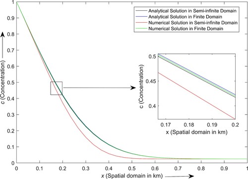
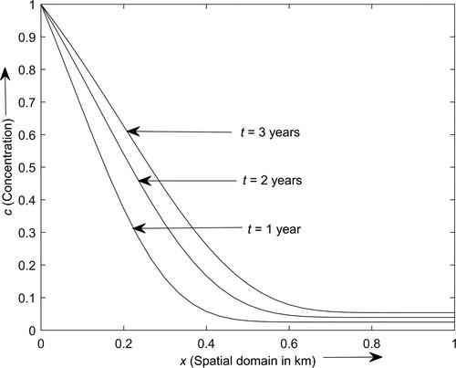
Figure 4 depicts the contaminant concentration distribution profiles at the time period levels $t=1,2,\text{and}3$ years in a semi-infinite gravel medium under the consideration of linear sorption. From the input source location, where the concentration is at the highest level, the contaminant spreads through the porous medium and reaches the lowest level near the outlet boundary. The concentration distribution profiles attained minimum levels and became constant after 0.5, 0.65 and 0.72 km, respectively at $t=1,2,\text{and}3$ years. The contaminant concentration increases with time, whereas it decreases with distance. However, the increasing rate of the contaminant concentration decreases with time except near the extreme boundary. Also, larger variation is observed among the concentration profiles around the intermediate location in comparison to the locations of inlet and outlet boundaries.

Figure 4. Contaminant concentration distribution profiles at different time levels.

Figures 5 and 6 depict the contaminant concentration distribution profiles in the semi-infinite domain for different values of the advection coefficients (i.e. $u_0=0.02,0.07,0.12,0.20$) and dispersion coefficient (i.e. $D_0=0.03,0.05,0.07,0.12$), respectively. With the modest fluctuations in the advection and dispersion coefficients, the concentration levels vary significantly at each point of the domain up to 0.6 km and subsequently become constant. For any given fixed time, the concentration level increases with the increasing values of advection and dispersion coefficients, whereas it decreases with space.

Figure 5. Contaminant concentration distribution profiles for different flow velocity values.

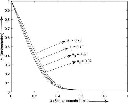
Figure 6. Contaminant concentration distribution profiles for different dispersion values.

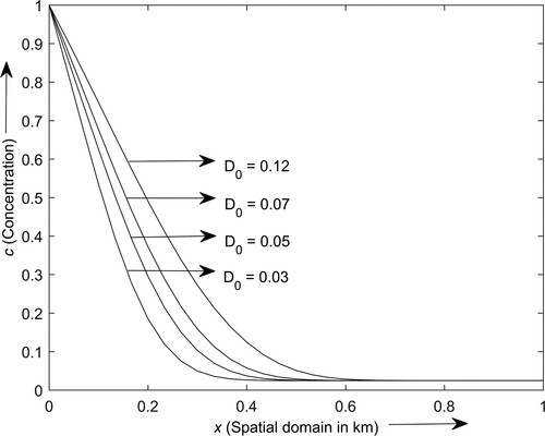
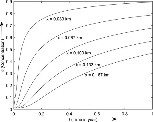
Figure 7 depicts the contaminant distribution concentration profiles in the semi-infinite domain at different spatial points for $t=1$ year. The contaminant concentration increases with time throughout the year at the spatial points near the inlet boundary. However, the concentration level decreases with space towards the outlet boundary. Also, a significant variation in the concentration profile nearest to the inlet boundary is observed throughout the year.

Figure 7. Contaminant concentration profiles with respect to time at some spatial points.

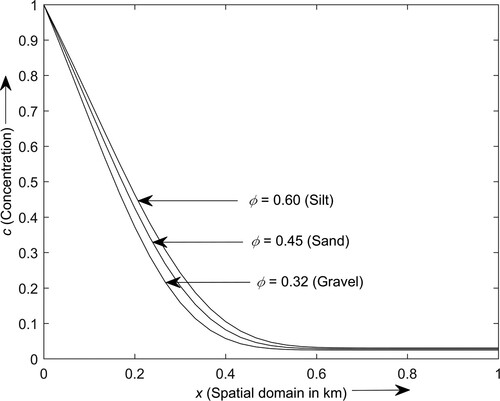
The distribution of the contaminant is affected by the porosity of the soil formations. Figure 8 depicts the contaminant transport behaviour in semi-infinite gravel, sand, and silt media obtained by analytical method at time $t=1$ year under the consideration of linear sorption. The contaminant concentration attains a maximum level in the silt medium and a minimum level in the gravel medium, thus implying that the contaminant concentration increases on increasing the porosity of the porous formation. Also, more considerable variation is observed among the concentration profiles as moving away from the inlet boundary up to the intermediate location, and beyond that, it becomes constant.

Figure 8. Contaminant concentration distribution profiles in different porous media.

The sorption induces a degradation effect on the contaminant fate and transport. The effect of sorption coefficient under the linear sorption on the contaminant transport is shown in Figure 9. The figure depicts the contaminant transport behaviour for different values of the sorption coefficient, i.e. $k_d=0.15,0.25,0.35$ at time $t=1$ year in the semi-infinite gravel medium. The contaminant concentration increases significantly on increasing the value of sorption coefficient except near the outlet boundary. A significant variation is observed among the concentration profiles around the intermediate location. It is also observed that the solute concentration increasing rate increases with the sorption coefficient.

Figure 9. Contaminant concentration distribution profiles for different values of sorption coefficient.

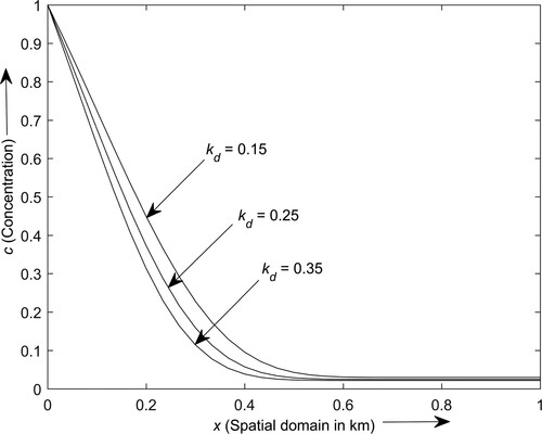
Figure 10 depicts the contaminant transport behaviour for different values of the non-linearity power i.e. $\omega =0,0.4,0.7,1$ at time $t=1$ year in the semi-infinite gravel medium obtained by numerical method. As sorption induces retardation, the contaminant concentration attains a lower level under the influence of sorption in comparison to the contaminant distribution without sorption. The contaminant concentration increases on increasing the value of non-linearity power. The variation in the concentration distribution profiles under the influence of sorption isotherm was found substantially less near the inlet and outlet boundaries than at the intermediate location. Also, a significant difference is observed between the contaminant concentration profiles obtained for non-linear sorption and without sorption.

Figure 10. Contaminant concentration distribution profiles for different values of the non-linearity power.

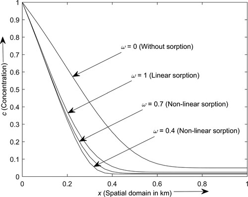
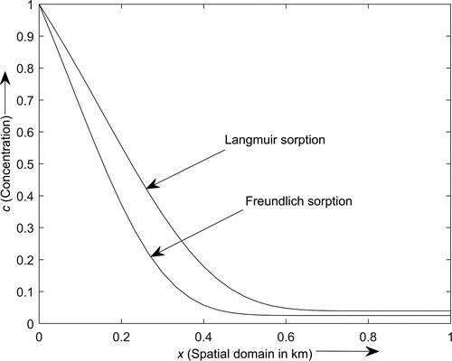
Figure 11 depicts the contaminant transport profiles in the semi-infinite domain for Freundlich and Langmuir sorption isotherms at $t=1$ year. The contaminant distribution profile attains a higher concentration level under the Langmuir sorption in comparison to the Freundlich sorption. The contaminant distribution profile under the Langmuir sorption may be more realistic than the Freundlich sorption; since, in the case of Langmuir sorption, there is an upper limit on the solid phase concentration to be sorbed onto the solid soil matrix.

Figure 11. Contaminant concentration distribution profiles for Langmuir and Freundlich sorption.

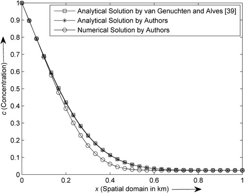
The accuracy of the numerical solution is examined by comparing it with the analytical solution under a special case. The numerical and analytical solutions are obtained for linear sorption isotherm subject to the steady-state flow at $t=1\text{ year}$ in the semi-infinite gravel medium, as shown in Figure 12. The graphical representations of the analytical solutions are obtained from this study as well as from the existing literature [39]. Both the analytical solutions coincide with each other. The numerical solution converges with the analytical solutions except around the intermediate location where minor variation is observed. Also, the numerical solution graph follows the same graphical pattern as the analytical solutions.

Figure 12. Comparison of analytical and numerical solutions under the special case.

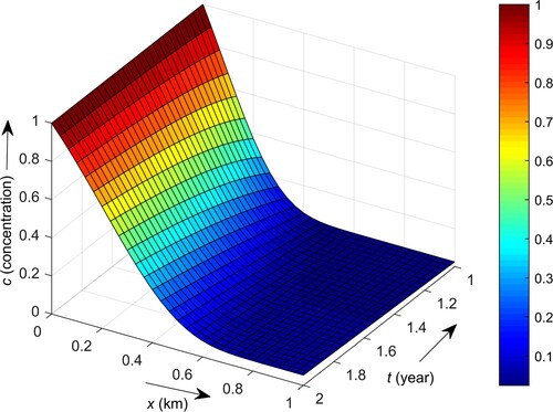
The contaminant concentration spreading profile in the semi-infinite domain is also shown graphically with respect to space and time. Figure 13 depicts the concentration spreading profile with respect to space and time. The contaminant concentration rises with time, whereas it decays with space. The contaminant concentration has a maximum level at the inlet boundary, decays with space, and attains a minimum level near the outlet boundary. The concentration decreases with space and attained minimum level around 0.6 km and then becomes constant towards the final boundary.

Figure 13. Contaminant distribution profile with respect to space and time.

For evaluation of the proposed model in terms of contaminant concentration prediction accuracy at different spatial points, the widely used root mean square (RMS) error metric is used, which is given as follows [47]: $\text{RMSE}=\left[\sqrt{\frac{\sum _{i=1}^n{\left(c_i^{\text{analytical}}-c_i^{\text{numerical}}\right)}^2}{n}}\right]$where, $i=1,2,\dots ,n$ is the number of observation points.

Table 1 shows the RMS errors and CPU runtimes for contaminant concentration distribution values at 16 spatial points in semi-infinite and finite porous domains obtained by numerical and analytical methods for different configurations of spatio-temporal grid size. A combination of spatial grid size of $\Delta x=0.0\text{333}$, $0.0167$ and temporal grid of $\Delta t=0.0\text{2}$, $0.01$ is chosen for illustrative purposes. The analytical and numerical results are obtained under linear sorption and uniform flow conditions with the help of MATLAB R2013 computing platform running on an intel COREi5 processor. As evident from Table 1, the overall RMS errors of the numerical solutions obtained in semi-infinite and finite domains are substantially less. However, compared to the finite domain, the error for the semi-infinite domain is comparatively larger. Moreover, altering the spatio-temporal grid resolution does not affect the accuracy of the solutions in the semi-infinite domain, whereas increasing the temporal grid size improves the accuracy in the finite domain. The CPU runtime of the analytical and numerical solutions are similar for coarse spatio-temporal grid size, while, as expected, increasing the grid resolution increases the CPU runtime.

Table 1. CPU runtimes and RMS errors of the numerical solutions with respect to the analytical solutions in semi-infinite and finite domains under the various discretization parameters.

	Semi-infinite domain				Finite domain
	Analytical solution	Numerical solution	Numerical solution	Numerical solution	Analytical solution	Numerical solution	Numerical solution	Numerical solution
Distance $x$ (in km)	$\begin{array}{l}\Delta x=0.0\text{333}\\ \Delta t=0.0\text{2}\end{array}$	$\begin{array}{l}\Delta x=0.0\text{333}\\ \Delta t=0.0\text{2}\end{array}$	$\begin{array}{l}\Delta x=0.0\text{167}\\ \Delta t=0.0\text{2}\end{array}$	$\begin{array}{l}\Delta x=0.0333\\ \Delta t=0.01\end{array}$	$\begin{array}{l}\Delta x=0.0\text{333}\\ \Delta t=0.0\text{2}\end{array}$	$\begin{array}{l}\Delta x=0.0\text{333}\\ \Delta t=0.0\text{2}\end{array}$	$\begin{array}{l}\Delta x=0.0\text{167}\\ \Delta t=0.0\text{2}\end{array}$	$\begin{array}{l}\Delta x=0.0333\\ \Delta t=0.01\end{array}$
0	1.0000	1.0000	1.0000	1.0000	1.0000	1.0000	1.0000	1.0000
0.0667	0.7914	0.7915	0.7882	0.7920	0.7931	0.7917	0.7919	0.7923
0.1333	0.5906	0.5789	0.5726	0.5800	0.5952	0.593	0.5931	0.5940
0.2000	0.4171	0.3845	0.3763	0.3858	0.4224	0.4198	0.4199	0.4211
0.2667	0.2796	0.2285	0.2201	0.2297	0.2842	0.2819	0.2817	0.2831
0.3333	0.1794	0.1216	0.1149	0.1225	0.1828	0.1811	0.1807	0.1822
0.4000	0.1123	0.0616	0.0574	0.0621	0.1145	0.1134	0.1129	0.1142
0.4667	0.0708	0.0352	0.0333	0.0354	0.0721	0.0716	0.0711	0.0722
0.5333	0.0473	0.0267	0.0261	0.0268	0.0479	0.0478	0.0474	0.0481
0.6000	0.0349	0.0249	0.0248	0.0249	0.0353	0.0353	0.0350	0.0355
0.6667	0.029	0.0246	0.0246	0.0246	0.0291	0.0292	0.0290	0.0293
0.7333	0.0263	0.0246	0.0246	0.0246	0.0264	0.0265	0.0263	0.0265
0.8000	0.0252	0.0246	0.0246	0.0246	0.0253	0.0253	0.0252	0.0253
0.8667	0.0248	0.0246	0.0246	0.0246	0.0248	0.0249	0.0248	0.0249
0.9333	0.0247	0.0246	0.0246	0.0246	0.0247	0.0247	0.0247	0.0247
1.0000	0.0246	0.0246	0.0246	0.0246	0.0246	0.0247	0.0247	0.0247
CPU runtime (in second)	0.1170	0.1400	0.1984	0.1606	0.1290	0.1390	0.1533	0.2583
RMSE		0.0269	0.0303	0.0264		0.0011	0.0013	0.0006

Summary and conclusions

The one-dimensional contaminant transport through a heterogeneous groundwater system is solved under the consideration of non-linear sorption, FOD, and ZOP. For the numerical solution, the CN scheme is applied successfully to approximate the non-linear governing equation. Also, the analytical solution is obtained in semi-infinite and finite domains subject to linear sorption and steady-state flow. A close agreement is observed between the exact and approximate solutions obtained in this study. Also, it is observed that the numerical solution obtained for the finite domain produces a marginal error than the numerical solution obtained for the semi-infinite domain. The contaminant concentration rises with time, whereas it decays with space. In the case of non-linearity power, the contaminant concentration rises with the increasing value of the non-linearity power. The retardation of the contaminant concentration is observed under the influence of sorption. Moreover, the solute concentration rises on increasing the sorption coefficient. A quantitative analysis of the performance of the proposed numerical model shows that the CPU run times are less while the RMS errors are marginal in the finite and semi-infinite domain. However, the RMS error of the numerical solution in the finite domain is observed to be lesser than the error obtained in the case of semi-infinite domain. The numerical solution obtained in this study has a marginal error; thus, it may be used to validate the analytical or numerical solutions obtained under the consideration of non-linear sorption isotherm. Further, this study may be extended to deal with non-equilibrium sorption.

Acknowledgements

The authors are thankful to the Indian Institute of Technology (Indian School of Mines), Dhanbad, for providing financial assistance through the JRF scheme. This work is also partially supported by the DST (SERB) Project EMR/2016/001628.

Disclosure statement

No potential conflict of interest was reported by the author(s).

Data availability statement

Some or all data, models, or code that support the findings of this study are available from the corresponding author upon reasonable request.

Additional information

Funding

The first author is financially supported by the Indian Institute of Technology (Indian School of Mines), Dhanbad, under the JRF scheme and partially by the Department of Science and Technology (Science and Engineering Research Board, New Delhi) Project EMR/2016/001628.

References

- Aral MM, Taylor SW. Groundwater quantity and quality management. Am Soc Civil Eng. 2011. https://doi.org/10.1061/9780784411766.
- van Genuchten MT. Analytical solutions for chemical transport with simultaneous adsorption, zero-order production and first-order decay. J Hydrol. 1981;49(3-4):213–233. DOI:10.1016/0022-1694(81)90214-6.
- Yates SR. An analytical solution for one-dimensional transport in porous media with an exponential dispersion function. Water Resour Res. 1992;28(8):2149–2154. DOI:10.1029/92WR01006.
- Serrano SE. Propagation of non-linear reactive contaminants in porous media. Water Resour Res. 2003;39(8):1288. DOI:10.1029/2002WR001922.
- Guerrero JP, Skaggs TH. Analytical solution for one-dimensional advection-dispersion transport equation with distance-dependent coefficients. J Hydrol. 2010;390(1-2):57–65. DOI:10.1016/j.jhydrol.2010.06.030.
- Kumar A, Jaiswal DK, Kumar N. One-dimensional solute dispersion along unsteady flow through a heterogeneous medium, dispersion being proportional to the square of velocity. Hydrol Sci J. 2012;57(6):1223–1230. DOI:10.1080/02626667.2012.695871.
- van Genuchten MTH, Leij FJ, Skaggs TH, et al. Exact analytical solutions for contaminant transport in rivers 1. The equilibrium advection-dispersion equation. J Hydrol Hydromech. 2013;61(2):146–160. DOI:10.2478/johh-2013-0020.
- Guerrero JP, Pontedeiro EM, van Genuchten MT, et al. Analytical solutions of the one-dimensional advection-dispersion solute transport equation subject to time-dependent boundary conditions. Chem Eng J. 2013;221:487–491. DOI:10.1016/j.cej.2013.01.095.
- Wadi AS, Dimian MF, Ibrahim FN. Analytical solutions for one-dimensional advection–dispersion equation of the pollutant concentration. J Earth Syst Sci. 2014;123(6):1317–1324.
- Hayek M. Analytical model for contaminant migration with time-dependent transport parameters. J Hydrol Eng. 2016;21(5):04016009. DOI:10.1061/(ASCE)HE.1943-5584.0001360.
- Purkayastha S, Kumar B. Analytical solution of the one-dimensional contaminant transport equation in groundwater with time-varying boundary conditions. Ish J Hydraul Eng. 2018;26(1):78–83. DOI:10.1080/09715010.2018.1453879.
- Molati M, Murakawa H. Exact solutions of non-linear diffusion-convection-reaction equation: a Lie symmetry analysis approach. Commun Nonlinear Sci Numer Simul. 2019;67:253–263. DOI:10.1016/j.cnsns.2018.06.024.
- Megahed AM, Reddy MG, Abbas W. Modeling of MHD fluid flow over an unsteady stretching sheet with thermal radiation, variable fluid properties and heat flux. Math Comput Simul. 2021;185:583–593.
- Megahed AM, Reddy MG. Numerical treatment for MHD viscoelastic fluid flow with variable fluid properties and viscous dissipation. Indian J Phys. 2021;95(4):673–679.
- Nasr ME, Gnaneswara Reddy M, Abbas W, et al. Analysis of non-linear radiation and activation energy analysis on hydromagnetic Reiner–Philippoff fluid flow with Cattaneo–Christov double diffusions. Mathematics. 2022;10(9):1534.
- Reddy MG, Kumar KG. Cattaneo-Christov heat flux feature on carbon nanotubes filled with micropolar liquid over a melting surface: a stream line study. Int Commun Heat Mass Transfer. 2021;122:105142.
- Reddy MG, Shehzad SA. Molybdenum disulfide and magnesium oxide nanoparticle performance on micropolar Cattaneo-Christov heat flux model. Appl Math Mech. 2021;42(4):541–552.
- Bosma WJP, van Der Zee SE. Transport of reacting solute in a one-dimensional, chemically heterogeneous porous medium. Water Resour Res. 1993a;29:117–131. DOI:10.1029/92WR01859.
- Dehghan M. Weighted finite difference techniques for the one-dimensional advection-diffusion equation. Appl Math Comput. 2004;147(2):307–319. DOI:10.1016/S0096-3003(02)00667-7.
- Fares YR, Giacobbe D. Transient transport of reactive and non-reactive solutes in groundwater. Comput Geosci. 2004;30(5):483–492. DOI:10.1016/j.cageo.2004.03.003.
- Maraqa MA. Retardation of nonlinearly sorbed solutes in porous media. J Environ Eng. 2007;133(6):587–594. DOI:10.1061/(ASCE)0733-9372(2007)133:6(587).
- Savović S, Djordjevich A. Finite difference solution of the one-dimensional advection-diffusion equation with variable coefficients in semi-infinite media. Int J Heat Mass Transf. 2012;55(15-16):4291–4294. DOI:10.1016/j.ijheatmasstransfer.2012.03.073.
- Savović S, Djordjevich A. Numerical solution for temporally and spatially dependent solute dispersion of pulse type input concentration in semi-infinite media. Int J Heat Mass Transf. 2013;60:291–295. DOI:10.1016/j.ijheatmasstransfer.2013.01.027.
- Gharehbaghi A. Explicit and implicit forms of differential quadrature method for advection-diffusion equation with variable coefficients in semi-infinite domain. J Hydrol. 2016;541:935–940. DOI:10.1016/j.jhydrol.2016.08.002.
- Mojtabi A, Deville MO. One-dimensional linear advection-diffusion equation: analytical and finite element solutions. Comput Fluids. 2015;107:189–195. DOI:10.1016/j.compfluid.2014.11.006.
- Gorokhovski V, Trofimov V. Advective solute transport through porous media along streamlines. Model Earth Syst Environ. 2017;3(3):839–860. DOI:10.1007/s40808-017-0313-0.
- Moranda A, Cianci R, Paladino O. Analytical solutions of one-dimensional contaminant transport in soils with source production-decay. Soil Syst. 2018;2(3):40. DOI:10.3390/soilsystems2030040.
- Li X, Zhan H, Wen Z. Impact of transient flow on subsurface solute transport with exponentially time-dependent flow velocity. J Hydrol Eng. 2018;23(7):04018030. DOI:10.1061/(ASCE)HE.1943-5584.0001679.
- Yadav RR, Roy J. Solute transport phenomena in a heterogeneous semi-infinite porous media: an analytical solution. Int J Appl Comput Math. 2018;4(6):1–14. DOI:10.1007/s40819-018-0567-x.
- Das P, Singh MK. One-dimensional solute transport with time-varying dispersion in porous formulation. J Porous Media. 2019;22(10):1207–1227. DOI:10.1615/JPorMedia.2019025964.
- Singh MK, Singh RK, Pasupuleti S. Study of forward-backward solute dispersion profiles in a semi-infinite groundwater system. Hydrol Sci J. 2020;65(8):1416–1429. DOI:10.1080/02626667.2020.1740706.
- Banaei SMA, Javid AH, Hassani AH. Numerical simulation of groundwater contaminant transport in porous media. Int J Environ Sci Technol. 2021;18(1):151–162. DOI:10.1007/s13762-020-02825-7.
- Naveen BP, Sumalatha J, Malik RK. A study on contamination of ground and surface water bodies by leachate leakage from a landfill in Bangalore, India. International J Geo Eng. 2018; 9(1):1–20. DOI:10.1186/s40703-018-0095-x.
- Andallah LS, Khatun MR. Numerical solution of advection-diffusion equation using finite difference schemes. Bangladesh J Sci Ind Res. 2020;55(1):15–22.
- Anley EF, Zheng Z. Finite difference approximation method for a space fractional convection–diffusion equation with variable coefficients. Symmetry. 2020;12(3):485.
- Fadugba SE, Edogbanya OH, Zelibe SC. Crank nicolson method for solving parabolic partial differential equations. IJA2M. 2013;1(3):8–23.
- Yadav RR, Roy J. Numerical solution for one-dimensional solute transport with variable dispersion. Environ Earth Sci Res J. 2019;6(1):35–42. DOI:10.18280/eesrj.060105.
- Zhang X, Zhu Y, Wang J, et al. GW-PINN: a deep learning algorithm for solving groundwater flow equations. Adv Water Res. 2022;165:104243.
- van Genuchten MTH, Alves WJ. Analytical solutions of the one dimensional convective-dispersive solute transport equation. Technical Bulletin No. 1661. United States Department of Agriculture, 151; 1982.
- Batu V. Applied flow and solute transport modeling in aquifers: fundamental principles and analytical and numerical methods. Boca Raton (FL): CRC Press; 2005.
- Bosma WJP, van Der Zee SE. Analytical approximation for non-linear adsorbing solute transport and first-order degradation. Transp Porous Media. 1993b;11(1):33–43. DOI:10.1007/BF00614633.
- Weber WJ, McGinley PM, Katz LE. Sorption phenomena in subsurface systems: concepts, models and effects on contaminant fate and transport. Water Res. 1991;25(5):499–528. DOI:10.1016/0043-1354(91)90125-A.
- Zheng C, Bennett GD. Applied contaminant transport modeling (Vol. 2). New York: Wiley-Interscience; 2002.
- Kumar A, Jaiswal DK, Kumar N. Analytical solutions to one-dimensional advection-diffusion equation with variable coefficients in semi-infinite media. J Hydrol. 2010;380(3-4):330–337. DOI:10.1016/j.jhydrol.2009.11.008.
- Freeze RA, Cherry JA. Groundwater. Englewood Cliffs: Prentice-Hall; 1979.
- Singh MK, Kumari P. Contaminant concentration prediction along unsteady groundwater flow. In: S Basu, N Kumar, editor. Modelling and simulation of diffusive processes; simulation foundations, methods and applications. Cham: Springer; 2014. p. 257–275. DOI:10.1007/978-3-319-05657-9_12
- Moriasi DN, Arnold JG, Van Liew MW, et al. Model evaluation guidelines for systematic quantification of accuracy in watershed simulations. Trans ASABE. 2007;50(3):885–900.