Existence, uniqueness and stability of solutions to fractional backward stochastic differential equations

ABSTRACT

Many types of fractional stochastic differential equation (FrSDE), such as Caputo, fractional Brown motion derivatives, and Mittag-Later functions, exist. In recent decades, FrSDE has been a hot topic and can be applied to many fields of research, such as disease transmission, option pricing, and quantitative finance. FrSDEs have various research and applications in financial markets. After comparing many internationally known articles, the fractional order stochastic differential equation proposed in 2016 is most suitable for European option pricing. Over the years, many scholars have studied fractional Brownian motion, fractional ordinary differential equations, and backward differential equations, and no one has studied the application of fractional backward equations in the financial field. Therefore, in this article, to adapt to the financial market more accurately, we construct a backward equation for this kind of FrSDE and construct a new mapping and use the norm method to prove the existence, uniqueness, and stability of the solution to the backward equation. Finally, considering European call options, the Euler Maruyama simulation example of FrSDE is investigated.

KEYWORDS:

• Fractional stochastic differential equation
• backward iteration
• existence and uniqueness
• stability

MATHEMATICS SUBJECT CLASSIFICATIONS:

• 60H35
• 65C20
• 60H10

1. Introduction

Time series with memory have been widely used in the fields of physics, chemistry, finance and biology. In this paper, we mainly consider that the time series of financial variables must be the memory dependent in the actual financial market. The financial variables here include a region's GDP, interest rate, foreign exchange, stock price, option price, and so on. The conditional probability method can be used to prove the existence of memory effect in stock price series, and the degree of long memory auto-correlation can also be measured [1,2].

Backward stochastic differential equation (BSDE) has developed rapidly in recent years, has been studied and applied in different fields such as probability and statistics, partial differential equation (PDE), function analysis, numerical analysis and stochastic calculation, engineering, economy and mathematical finance. It is impossible for us to give a complete review of all important developments in the past 20 years. The most classic work is the literature [3], in which readers can consult on their own. Therefore, we mainly introduce the method of fractional differential equation, analyse the existence and uniqueness of its solution by using the backward thinking, and finally attempt to evaluate the effect of its numerical solution.

In recent decades, fractional order stochastic differential equation has been a popular topic and can be applied to many fields of research, such as disease transmission, option pricing, and quantitative finance [4–7]. There are two primary research directions: stochastic differential equation driven by fractional Brownian motion (FbmSDE) and stochastic differential equation with Caputo fractional derivatives (Caputo-FrSDE). The form of FbmSDE [8] is represented as follows Equation(1(1) $\begin{array}{r}\mathrm{d}{X}_t=b(t,X_t)\mathrm{d}t+\sigma (t)\mathrm{d}{W}_t^H,X_0=x_0.\end{array}$(1) ): (1) $\begin{array}{r}\mathrm{d}{X}_t=b(t,X_t)\mathrm{d}t+\sigma (t)\mathrm{d}{W}_t^H,X_0=x_0.\end{array}$(1) In the formula, $X_t$ represents the stock price in time t, $b(t,X_t)$ represents drift coefficient that changes with stock price and time, $\sigma (t)$ represents the volatility that changes with time, and $W_t^H$ represents the Fractional Brownian motion.

Although fractional Brownian motion has lost its martingale property, it will obtain Brownian motion with memory trend according to the Hurst exponent(H) [1]. FbmSDE also has many applications in finance [8]. After Peng [3] proposed the backward equation of FbmSDE: $\mathrm{d}{y}_t=-[{\beta }_t{y}_t+{\gamma }_t{z}_t]\mathrm{d}t-z_t\mathrm{d}{B}_t^h$, ELS options can now be priced [9].

The second type is Caputo-SDE. A new derivative is defined by Caputo as Equation(2(2) $\begin{array}{r}\frac{{\mathrm{d}}^{m+z}}{\mathrm{d}{t}^{m+z}}f(t)=\frac{1}{\mathrm{\Gamma }(1-z)}{\int }_0^t(t-\xi {)}^{-z}{f}^{(m+1)}(\xi )\mathrm{d}\xi .\end{array}$(2) ) [10]: (2) $\begin{array}{r}\frac{{\mathrm{d}}^{m+z}}{\mathrm{d}{t}^{m+z}}f(t)=\frac{1}{\mathrm{\Gamma }(1-z)}{\int }_0^t(t-\xi {)}^{-z}{f}^{(m+1)}(\xi )\mathrm{d}\xi .\end{array}$(2) In the equatoion, $\mathrm{\Gamma }(\cdot )$ represents the gamma function.

Because the processes of the financial market have random effects, Li et al. [9] added the random process to fractional ordinary differential equation (Caputo-Li FrSDE) and proposed a new model constructed from fractional stochastic differential equation [11]. The stochastic process of asset price expressed by the fractional stochastic differential equation is as follows: (3) $\begin{array}{r}{\mathrm{d}}^{\alpha }x=\mu (x,t)\mathrm{d}{t}^{\alpha }+\sigma (x,t)\mathrm{d}B(t),\alpha =2H.\end{array}$(3) In Equation(3(3) $\begin{array}{r}{\mathrm{d}}^{\alpha }x=\mu (x,t)\mathrm{d}{t}^{\alpha }+\sigma (x,t)\mathrm{d}B(t),\alpha =2H.\end{array}$(3) ), H is the Hurst index, which describes the memory of the time series and can be calculated by R/SD. In the special case of $\alpha =1(i.e.H=0.5)$, the equation is simplified to a classical stochastic differential equation. H will change the integral form of SDE. In other papers, the finite time stability of solutions of linear stochastic fractional order systems with time delay is also studied when $H\in (\frac{1}{2},1)$ [12]. However, only $H\in (\frac{1}{2},1)$ can be considered in the financial market. Inspired by the above literature, we proposes a backward SDE in this range in the form of: (4) $\begin{array}{r}{Y}_t=Y_T+{\int }_t^{T}f(s)[\frac{\alpha \cdot (T-s{)}^{x^{\alpha -1}}}{\mathrm{\Gamma }(1+\alpha )}-1]\mathrm{d}s-{\int }_t^T\frac{z(s,T)}{\mathrm{\Gamma }(1+\alpha )}\mathrm{d}{B}_s,\alpha \in (1,2).\end{array}$(4) We mainly introduce a new norm to verify the existence and uniqueness of solutions of above backward fractional differential equations. In the current academic research process, some people have studied the backward equation and fractional differential equation, but no one has studied the subject of this paper, so it is a relatively new idea.

The paper is organized as follows. In Second 2, we introduce the transformation from Caputo fractional reciprocal to fractional differential equation. In Section 3, some hypotheses and lemmas are proposed to facilitate the later theorem citation. In Section 4, the existence and uniqueness of mild solutions of backward fractional differential equations are proven, and the interval conditions for the existence of solutions are given. In Section 5, stability conditions of the backward fractional differential equations are given. In Section 6, the Euler simulation solution of fractional SDE is simply compared with the real solution under specific circumstances. In Section 7, we conclude our investigation.

2. Fractional backward stochastic integral equation

In the real financial market, the Hurst index typically only considers the case that $H\in (\frac{1}{2},1)$, the following research is based on this premise. In this interval, the Caputo fractional derivative is in the following form [11]: (5) $\begin{array}{r}{\mathrm{d}}^{\alpha }f=\mathrm{\Gamma }(1+\alpha )[\mathrm{d}f-f^{\mathrm{\prime }}(x)\mathrm{d}x].\end{array}$(5) In addition, let $Y=g(X)$, X is the stock price. The drift coefficient is changed from $\mu (X,t)$ to $f(t,Y_t,Z_t)$, and the fluctuation coefficient is changed from $\sigma (X,t)$ to $Z(t)$. We substitute this variable into Equation(3(3) $\begin{array}{r}{\mathrm{d}}^{\alpha }x=\mu (x,t)\mathrm{d}{t}^{\alpha }+\sigma (x,t)\mathrm{d}B(t),\alpha =2H.\end{array}$(3) ) and obtain: (6) $\begin{array}{r}{\mathrm{d}}^{\alpha }{Y}_t=f(t,Y_t,Z_t)(\mathrm{d}t{)}^{\alpha }+Z_t\mathrm{d}t.\end{array}$(6) Combining with Equations(5(5) $\begin{array}{r}{\mathrm{d}}^{\alpha }f=\mathrm{\Gamma }(1+\alpha )[\mathrm{d}f-f^{\mathrm{\prime }}(x)\mathrm{d}x].\end{array}$(5) ) and(6(6) $\begin{array}{r}{\mathrm{d}}^{\alpha }{Y}_t=f(t,Y_t,Z_t)(\mathrm{d}t{)}^{\alpha }+Z_t\mathrm{d}t.\end{array}$(6) ), we obtain: (7) $\begin{array}{r}\mathrm{d}{Y}_t=\frac{f(t,Y_t,Z_t)}{\mathrm{\Gamma }(1+\alpha )}(\mathrm{d}t{)}^{\alpha }+\frac{Z_t}{\mathrm{\Gamma }(1+\alpha )}\mathrm{d}{B}_t+Y^{\mathrm{\prime }}(t)\mathrm{d}t.\end{array}$(7) Notice that $(Y_t^{\mathrm{\prime }})\mathrm{d}t=m(t),m(t)$ represents the daily returns of stock $f(t,Y_t,Z_t)$, and $m(t)=$ $f(t,Y_t,Z_t)\mathrm{d}t,f(t,Y_t,Z_t)$ is the returns of one year; thus, $Y_t^{\mathrm{\prime }}=f(t,Y_t,Z_t)$, and Equation(7(7) $\begin{array}{r}\mathrm{d}{Y}_t=\frac{f(t,Y_t,Z_t)}{\mathrm{\Gamma }(1+\alpha )}(\mathrm{d}t{)}^{\alpha }+\frac{Z_t}{\mathrm{\Gamma }(1+\alpha )}\mathrm{d}{B}_t+Y^{\mathrm{\prime }}(t)\mathrm{d}t.\end{array}$(7) ) can be written as follows: (8) $\begin{array}{r}\mathrm{d}{Y}_t=\frac{f(t,Y_t,Z_t)}{\mathrm{\Gamma }(1+\alpha )}(\mathrm{d}t{)}^{\alpha }+\frac{Z_t}{\mathrm{\Gamma }(1+\alpha )}\mathrm{d}{B}_t+f(t,Y_t,Z_t)\mathrm{d}t.\end{array}$(8) Integrating Equation(8(8) $\begin{array}{r}\mathrm{d}{Y}_t=\frac{f(t,Y_t,Z_t)}{\mathrm{\Gamma }(1+\alpha )}(\mathrm{d}t{)}^{\alpha }+\frac{Z_t}{\mathrm{\Gamma }(1+\alpha )}\mathrm{d}{B}_t+f(t,Y_t,Z_t)\mathrm{d}t.\end{array}$(8) ) in the interval $[t,T]$ and noting that ${\int }_0^{t}f(s)(\mathrm{d}s{)}^{\alpha }=\alpha (\alpha -1){\int }_0^t(t-s{)}^{\alpha -2}F(s)\mathrm{d}s,F(s)={\int }_0^{s}f(r)\mathrm{d}r,$we take the backward equation according to the method from [13], to obtain the result: (9) $\begin{array}{rl}{Y}_t& =g(X_T)+{\int }_t^T[\frac{\alpha \cdot (\alpha -1)\cdot (T-s{)}^{\alpha -2}}{\mathrm{\Gamma }(1+\alpha )}-1]F(s,Y_s,Z_s)\mathrm{d}s\\ & -{\int }_t^T\frac{Z(s,T)}{\mathrm{\Gamma }(1+\alpha )}\mathrm{d}Bs,g(X_T)=Y_T.\end{array}$(9)

3. Assumptions and conditions

In this section, we primarily build some lemmas and conditional assumptions to facilitate the proof of theorems in the next sections.

Assumption 3.1

First of all, we denote by $L_T^2({\mathbf{R}}^d)$ the set of ${\mathcal{F}}_T$-measurable random variables X: $\mathrm{\Omega }\to {\mathbf{R}}^d$ which are square integrable, and by ${\mathcal{H}}_T^2({\mathbf{R}}^a)$ the set of predictable processes $\eta :\mathrm{\Omega }\times [0,T]\to {\mathbf{R}}^a$ such that $\mathbb{E}\left[{\int }_0^T{\left|{\eta }_t\right|}^2\mathrm{d}t\right]<\mathrm{\infty }.$where $|\cdot |$ the standard Euclidean norm in the Euclidean space ${\mathbf{R}}^a(a=1$, or q). The terminal condition $Y_T$ in Equation(9(9) $\begin{array}{rl}{Y}_t& =g(X_T)+{\int }_t^T[\frac{\alpha \cdot (\alpha -1)\cdot (T-s{)}^{\alpha -2}}{\mathrm{\Gamma }(1+\alpha )}-1]F(s,Y_s,Z_s)\mathrm{d}s\\ & -{\int }_t^T\frac{Z(s,T)}{\mathrm{\Gamma }(1+\alpha )}\mathrm{d}Bs,g(X_T)=Y_T.\end{array}$(9) ) is ${\mathcal{F}}_T$-measurable and square integrable. Moreover, we need the following assumptions [14]:

(A1)	For all $Y_t^1,Y_t^2\in {\mathbb{R}}^n,Z_t^1,Z_t^2\in {\mathbb{R}}^{n\times m}$ and $0\le t\le T$, there exists c>0 such that $\Vert g(t,s,X_t^1)-g(t,s,X_t^2){\Vert }^2\le c\Vert X_t^1-X_t^2{\Vert }^2\mathrm{a}.\mathrm{s}.$and $g(\cdot ,\cdot ,0)$ is essentially bounded, i.e. $ess\underset{r\in [0,T]}{sup}\Vert g(r,u,0)\Vert <\mathrm{\infty }.$
(A2)	The functions $\mu (x)$ and $\sigma (x)$ are uniformly Lipschitz continuous and satisfy linear growth condition.
(A3)	The generator $f(t,y,z)$ satisfies the following continuity condition: $\begin{array}{rl}& \Vert F(t,Y_t^1,Z_t^1)-F(t,Y_t^2,Z_t^2){\Vert }^2\le C_F(\Vert Y_t^1-Y_t^2{\Vert }^2+\Vert Z_t^1-Z_t^2{\Vert }^2),\mathrm{a}.\mathrm{s},\\ & {\int }_0^T\Vert F(r,0,0){\Vert }^2\mathrm{d}r<\mathrm{\infty }.\end{array}$for any $(t,y_2,z_2),(t,y_1,z_1)\in [0,T]\times \mathbf{R}\times {\mathbf{R}}^q$, where $C_F>0$ is a constant.

Lemma 3.1

Bohr's inequality [15]

If $(X,\parallel \cdot \parallel )$ is a normed linear space, when p, q>1 and $\frac{1}{p}+\frac{1}{q}=1$. Then, $\parallel x+y{\parallel }^2\le p\parallel x{\parallel }^2+q\parallel y{\parallel }^2,x,y\in X.$Also, $\Vert \sum _{i=1}^m{x}_i{\Vert }^2⩽m\sum _{i=1}^m\Vert x_i\Vert ,x_i\in X.$

Lemma 3.2

Jesson's inequality [15]

Suppose φ is a convex function in $[\alpha ,\beta ]$, f, p are integrable in $[a,b]$, α $⩽f(x)⩽\beta ,p(x)⩾0,x\in [a,b]$, and ${\int }_a^{b}p(x)\mathrm{d}x>0$.Then $\phi \left(\frac{{\int }_a^{b}p(x)f(x)\mathrm{d}x}{{\int }_a^{b}p(x)\mathrm{d}x}\right)⩽\frac{{\int }_a^{b}p(x)\phi [f(x)]\mathrm{d}x}{{\int }_a^{b}p(x)\mathrm{d}x}.$Specially, ${({\int }_a^{b}p(x)f(x)\mathrm{d}x)}^2\le {\int }_a^{b}p(x)f^2(x)\mathrm{d}x\cdot {\int }_a^{b}p(x)\mathrm{d}x.$

Lemma 3.3

Holder's inequality [15]

Suppose $a=(a_1,\dots ,a_n)$ or $a=(a_1,\dots ,a_n,\dots )$ is a real or imaginary column. Let $\Vert a{\Vert }_p=\{\begin{array}{ll}{\left(\sum _k{\left|a_k\right|}_p\right)}^{1/p},& 0<p<\mathrm{\infty },\\ \underset{k}{sup}\left|a_k\right|,& p=\mathrm{\infty },\end{array}$$\frac{1}{p}+\frac{1}{q}=1$, when p = 1, it is stipulated that $q=\mathrm{\infty }$, then $\Vert ab{\Vert }_1⩽\Vert a{\Vert }_p\Vert b{\Vert }_q.$Specially, $\Vert ab{\Vert }_1^2⩽\Vert a{\Vert }_2^2\cdot \Vert b{\Vert }_2^2.$

Lemma 3.4

Banach's theorem [16]

Suppose X is a metric space. $T:X\to X$ is a mapping (It does not have to be linear). There exists a constant $a(0\le a<1)$ such that $\mathrm{d}(Tx,Ty)\le a\cdot (x,y),\mathrm{\forall }x,y\in X.$Then, there exists $x\in X$ makes Tx = x, where T is a compression map.

Lemma 3.5

Martingale representation theorem [17]

Let $X(t),0\le t\le T$, be a local martingale adapted to the Brownian filtration ${\mathbb{F}}^B=({\mathcal{F}}_t)$. Then there exists a predictable process $H(t)$ such that ${\int }_0^T{H}^2(s)\mathrm{d}s<\mathrm{\infty }$ with probability 1, and the following equation holds $X(t)=X(0)+{\int }_0^{t}H(s)\mathrm{d}B(s).$Moreover, if Y is an integrable ${\mathcal{F}}_T$-measurable random variable, $\mathrm{E}|Y|<\mathrm{\infty }$, then $Y=\mathrm{E}Y+{\int }_0^{T}H(t)\mathrm{d}B(t).$If in addition, Y and B have jointly a Gaussian distribution, then the process $H(t)$ is deterministic.

Lemma 3.6

[15]

Suppose $u(t),b(t)\ge 0,t\in [t_0,T]$, and $u(t)\le a+{\int }_{t_0}^{T}b(s)\cdot u(s)\mathrm{d}s$. Thus $u(t)\le a\cdot exp[{\int }_{t_0}^{T}b(s)\mathrm{d}s],t\in [t_0,T].$

Definition 3.1

Let $1<\alpha <2$ and $1\le p<\mathrm{\infty }$ be fixed. We say that a measurable function $h:\mathrm{\Omega }\times [0,T]\to$ ${\mathbb{R}}^n$ belongs to ${\mathbb{L}}^{p,\alpha }([0,T],{\mathbb{R}}^n)$ if and only if the quantity $\Vert h{\Vert }_{p\cdot \alpha ,t}:=\underset{t\le m\le T}{\mathrm{Sup}}E{({\int }_t^m[\alpha \cdot (\alpha -1)(m-s{)}^{\alpha -2}-\mathrm{\Gamma }(1+\alpha )]\cdot \Vert h(s){\Vert }^p\mathrm{d}s)}^{\frac{1}{p}}<\mathrm{\infty }.$

Definition 3.2

The trivial solution of Equation(9(9) $\begin{array}{rl}{Y}_t& =g(X_T)+{\int }_t^T[\frac{\alpha \cdot (\alpha -1)\cdot (T-s{)}^{\alpha -2}}{\mathrm{\Gamma }(1+\alpha )}-1]F(s,Y_s,Z_s)\mathrm{d}s\\ & -{\int }_t^T\frac{Z(s,T)}{\mathrm{\Gamma }(1+\alpha )}\mathrm{d}Bs,g(X_T)=Y_T.\end{array}$(9) ) is said to be exponentially stable [18] in the quadratic mean if there exist positive constants C, v such that $\mathbb{E}(|Y(t){|}^2)\le C\mathbb{E}\left({\left|Y_0\right|}^2\right)\exp (-vt),t\ge 0.$

Lemma 3.7

Let $1<\alpha <2$ and $1\le p<\mathrm{\infty }$. Then, ${\mathbb{L}}^{p,\alpha }$ is a Banach space.

Proof.

Obviously, the defined weighted norm satisfies the conditions of norm in ${\mathbb{L}}^{p,\alpha }$ space. It is only left to show that it is complete. Hence, a proof of this part is similar to the proof of Theorem 3.4 in [19], so we omit it here.

In particular, we consider p = 2 and $1<\alpha <2$ throughout this paper such that the weighted norm is defined by $\Vert h{\Vert }_{2\cdot \alpha ,t}:=\underset{t\le m\le T}{\mathrm{Sup}}E{({\int }_t^m[\alpha \cdot (\alpha -1)(m-s{)}^{\alpha -2}-\mathrm{\Gamma }(1+\alpha )]\cdot \Vert h(s){\Vert }^2\mathrm{d}s)}^{\frac{1}{2}}.$To show existence and uniqueness of the solutions to backward fractional differential equation, we consider the following norm: $\Vert h{\Vert }_{2\cdot \alpha ,0}:=\underset{t\le m\le T}{\mathrm{Sup}}E{({\int }_0^m[\alpha \cdot (\alpha -1)(m-s{)}^{\alpha -2}-\mathrm{\Gamma }(1+\alpha )]\cdot \Vert h(s){\Vert }^2\mathrm{d}s)}^{\frac{1}{2}}.$We define $M[t,T]:={\mathbb{L}}_{\mathcal{F}}^2(t,T;{\mathbb{R}}^n)\times {\mathbb{L}}_{\mathcal{F}}^2(\mathcal{D};{\mathbb{R}}^{n\times m})$ to be a Banach space endowed with the norm $\Vert (y,z){\Vert }_t^2=\Vert y{\Vert }_{2,\alpha ,t}^2+{|\Vert z\Vert |}_{2,\alpha ,t}^2,$where ${|\Vert z\Vert |}_{2,\alpha ,t}=\underset{t\le m\le T}{\mathrm{Sup}}{\mathrm{Sup}}_{t\le m\le T}E{({\int }_t^m\alpha (\alpha -1)(m-s{)}^{{\alpha }^{\alpha -2}}\cdot ({\int }_t^s\Vert z{\Vert }^2\mathrm{d}x)\mathrm{d}s)}^{\frac{1}{2}}.$Then $M[0,T]:={\mathbb{L}}_{\mathcal{F}}^2(0,T;{\mathbb{R}}^n)\times {\mathbb{L}}_{\mathcal{F}}^2([0,T{]}^2;{\mathbb{R}}^{n\times m})$ is also Banach space equipped with the norm as below: $\Vert (y,z){\Vert }_0^2=\Vert x{\Vert }_{2,\alpha ,0}^2+{|\Vert z\Vert |}_{2,\alpha ,0}^2.$

4. Existence and uniqueness

To prove the existence and uniqueness theorem of solutions, we must first discuss the existence and uniqueness of solutions and find a range to make Banach's fixed point theorem hold. First, we prove Lemma 4.1 which is important in the next proof.

Lemma 4.1

For any $(y(\cdot ),z(\cdot ,\cdot ))\in M[t,T]$, FrBSDE equation (10) $\begin{array}{r}{Y}_t=Y_T+{\int }_t^T[\frac{\alpha \cdot (\alpha -1)\cdot (T-s{)}^{\alpha -2}}{\mathrm{\Gamma }(1+\alpha )}-1]F(s)\mathrm{d}s-{\int }_t^T\frac{Z(s,T)}{\mathrm{\Gamma }(1+\alpha )}\mathrm{d}Bs\end{array}$(10) admits a unique solution in $M[0,T]$.

Proof.

Uniqueness: Take expectations $E(\cdot |{\mathcal{F}}_t)$ on both sides of Equation(10(10) $\begin{array}{r}{Y}_t=Y_T+{\int }_t^T[\frac{\alpha \cdot (\alpha -1)\cdot (T-s{)}^{\alpha -2}}{\mathrm{\Gamma }(1+\alpha )}-1]F(s)\mathrm{d}s-{\int }_t^T\frac{Z(s,T)}{\mathrm{\Gamma }(1+\alpha )}\mathrm{d}Bs\end{array}$(10) ) at the same time. ${\mathcal{F}}_t$ represents the information we know at time t. Then we get: (11) $\begin{array}{r}{Y}_t=E(Y_T\mid {\mathcal{F}}_t)+{\int }_t^T[\frac{\alpha \cdot (\alpha -1)\cdot (T-s{)}^{\alpha -2}}{\gamma (1+\alpha )}-1]\cdot E(F(s)\mid {\mathcal{F}}_t)\mathrm{d}s.\end{array}$(11) Assuming that $(Y_t^1,Z_t^1)$ and $(Y_t^2,Z_t^2)$ are different solutions of Equation(10(10) $\begin{array}{r}{Y}_t=Y_T+{\int }_t^T[\frac{\alpha \cdot (\alpha -1)\cdot (T-s{)}^{\alpha -2}}{\mathrm{\Gamma }(1+\alpha )}-1]F(s)\mathrm{d}s-{\int }_t^T\frac{Z(s,T)}{\mathrm{\Gamma }(1+\alpha )}\mathrm{d}Bs\end{array}$(10) ), then $Y_t^1-Y_t^2={\int }_t^T\frac{Z_t^2-Z_t^1}{\mathrm{\Gamma }(1+\alpha )}\mathrm{d}{B}_s.$Thus $E\left({\int }_t^T\frac{Z_t^2-Z_t^1}{\mathrm{\Gamma }(1+\alpha )}\mathrm{d}{B}_s|{\mathcal{F}}_t\right)=0,$and $E(Y_t^1-Y_t^2|{\mathcal{F}}_t)=0(\mathrm{\forall }t\in (0,T)).$Thus $E(Y^1=Y^2|{\mathcal{F}}_t)\mathrm{a}.\mathrm{e}.$It is obvious that $Y^1=Y^2$ and this follows that $Z^1=Z^2$.

Existence: According to Equation(11(11) $\begin{array}{r}{Y}_t=E(Y_T\mid {\mathcal{F}}_t)+{\int }_t^T[\frac{\alpha \cdot (\alpha -1)\cdot (T-s{)}^{\alpha -2}}{\gamma (1+\alpha )}-1]\cdot E(F(s)\mid {\mathcal{F}}_t)\mathrm{d}s.\end{array}$(11) ), we find that $E(Y_T\mid {\mathcal{F}}_t)$ and $E(f(s)\mid {\mathcal{F}}_t)$ are unknown. According to Lemma 3.5, we know that $E(Y_T\mid {\mathcal{F}}_t)$ is a martingale. Thus we have ${\int }_0^T{H}^2(s)\mathrm{d}s<\mathrm{\infty },K(t,u)\in L_{{\mathcal{F}}_t}^2(\mathcal{D};L^2(R^{n\times m}))$ which make (12) $\begin{array}{r}\begin{array}{rl}& E(Y_T\mid {\mathcal{F}}_t)=E\left(Y_T\right)+{\int }_0^{T}H(s)\mathrm{d}Bs,\\ & E(F(s)\mid {\mathcal{F}}_t)=E(F(s))+{\int }_0^{T}K(s,u)\mathrm{d}{B}_u\end{array}\end{array}$(12) Obviously, for all $s\in [0,T]$, we have $K(s,\mu )=0$ when $\mu \in [s,T]$.

Because $\begin{array}{rl}{Y}_T& =E\left(Y_T\right)+{\int }_0^{T}L(u)\mathrm{d}Bu.\\ & =E\left(Y_T\right)+{\int }_0^{t}L(u)\mathrm{d}Bu+{\int }_t^{T}L(u)\mathrm{d}Bu\\ & =E(Y_T\mid f_t)+{\int }_t^{T}L(u)\mathrm{d}Bu,\end{array}$we have (13) $\begin{array}{r}E(Y_T\mid {\mathcal{F}}_t)=Y_T-{\int }_t^{T}L(u)\mathrm{d}Bu.\end{array}$(13) Similarly, (14) $\begin{array}{r}E(F(s)\mid {\mathcal{F}}_t)=F(s)-{\int }_t^{T}K(s,u)\mathrm{d}Bu.\end{array}$(14) Substitute Equations(13(13) $\begin{array}{r}E(Y_T\mid {\mathcal{F}}_t)=Y_T-{\int }_t^{T}L(u)\mathrm{d}Bu.\end{array}$(13) ) and(14(14) $\begin{array}{r}E(F(s)\mid {\mathcal{F}}_t)=F(s)-{\int }_t^{T}K(s,u)\mathrm{d}Bu.\end{array}$(14) ) into Equation(11(11) $\begin{array}{r}{Y}_t=E(Y_T\mid {\mathcal{F}}_t)+{\int }_t^T[\frac{\alpha \cdot (\alpha -1)\cdot (T-s{)}^{\alpha -2}}{\gamma (1+\alpha )}-1]\cdot E(F(s)\mid {\mathcal{F}}_t)\mathrm{d}s.\end{array}$(11) ), we have $\begin{array}{rl}{Y}_t& =Y_T-{\int }_t^{T}L(u)\mathrm{d}Bu+{\int }_t^T[\frac{\alpha \cdot (\alpha -1)(T-s{)}^{\alpha -2}}{\mathrm{\Gamma }(1+\alpha )}-1]\\ & \cdot [F(s)-{\int }_t^{s}k(s,u)\mathrm{d}Bu]\mathrm{d}s\\ & =Y_T-{\int }_t^{T}L(u)\mathrm{d}Bu+{\int }_t^T[\frac{\alpha \cdot (\alpha -1)(T-s{)}^{\alpha -2}}{\mathrm{\Gamma }(1+\alpha )}-1]F(s)\mathrm{d}s\\ & -{\int }_t^T[\frac{\alpha \cdot (\alpha -1)(T-s{)}^{\alpha -2}}{\mathrm{\Gamma }(1+\alpha )}-1]\cdot ({\int }_t^{s}K(s,u)\mathrm{d}Bu)\mathrm{d}s\\ & =Y_T+{\int }_1^T[\frac{\alpha \cdot (\alpha -1)(T-s{)}^{\alpha -2}}{\mathrm{\Gamma }(1+\alpha )}-1]F(s)\mathrm{d}s-{\int }_t^{T}L(u)\mathrm{d}Bu\\ & -{\int }_t^T[{\int }_u^T[\frac{\alpha \cdot (\alpha -1)(T-s{)}^{\alpha -2}}{\mathrm{\Gamma }(1+\alpha )}-1]\mu (u,s)\mathrm{d}s]\mathrm{d}Bu\\ & =Y_T+{\int }_t^T[\frac{\alpha \cdot (\alpha -1)(T-s{)}^{\alpha -2}}{\mathrm{\Gamma }(1+\alpha )}-1]F(s)\mathrm{d}s\\ & -{\int }_t^T[L(u)+{\int }_u^T[\frac{\alpha \cdot (\alpha -1)(T-s{)}^{\alpha -2}}{\mathrm{\Gamma }(1+\alpha )}-1]\cdot K(s,u)\mathrm{d}s]\mathrm{d}Bu.\end{array}$Compared with Equation(10(10) $\begin{array}{r}{Y}_t=Y_T+{\int }_t^T[\frac{\alpha \cdot (\alpha -1)\cdot (T-s{)}^{\alpha -2}}{\mathrm{\Gamma }(1+\alpha )}-1]F(s)\mathrm{d}s-{\int }_t^T\frac{Z(s,T)}{\mathrm{\Gamma }(1+\alpha )}\mathrm{d}Bs\end{array}$(10) ), we can get (15) $\begin{array}{r}Z(u,T)=\mathrm{\Gamma }(1+\alpha )L(u)+{\int }_u^T[\alpha \cdot (\alpha -1)(T-s{)}^{\alpha -2}-\mathrm{\Gamma }(1+\alpha )]\cdot K(s,u)\mathrm{d}s.\end{array}$(15) Then there exists a solution $(y,z)\in M[0,T]$ of Equation(10(10) $\begin{array}{r}{Y}_t=Y_T+{\int }_t^T[\frac{\alpha \cdot (\alpha -1)\cdot (T-s{)}^{\alpha -2}}{\mathrm{\Gamma }(1+\alpha )}-1]F(s)\mathrm{d}s-{\int }_t^T\frac{Z(s,T)}{\mathrm{\Gamma }(1+\alpha )}\mathrm{d}Bs\end{array}$(10) ) given by (16) $\begin{array}{r}{Y}_t=E(Y_T\mid {\mathcal{F}}_t)+{\int }_t^T[\frac{\alpha \cdot (\alpha -1)(T-s{)}^{\alpha -2}}{\mathrm{\Gamma }(1+\alpha )}-1]E(F(s)\mid {\mathcal{F}}_t)\mathrm{d}s.\end{array}$(16)

Next, let's find out the range that makes Banach's theorem true.

Lemma 4.2

(17) $\begin{array}{rl}{|\Vert z\Vert |}_{2\cdot \alpha \cdot t}^2+{\Vert Y_t\Vert }_{2,\alpha ,t}^2& \le 8{\mathrm{\Gamma }}^2(1+\alpha )\\ & \cdot {\int }_t^m[\alpha \cdot (\alpha -1)(T-s{)}^{\alpha -2}-\mathrm{\Gamma }(1+\alpha )]\cdot E{\Vert Y_t\Vert }^2\mathrm{d}s\\ & +{\mathcal{A}}_{\alpha ,T,t}\cdot \Vert F{\Vert }_{2,\alpha ,t}^2+2{\Vert E(Y_T\mid {\mathcal{F}}_t)\Vert }_{2,\alpha ,t}^2,\end{array}$(17) where $\begin{array}{rl}{\mathcal{A}}_{\alpha ,T,t}& =2\cdot (T-t{)}^2{[(T-t{)}^{\alpha -2}-\frac{\alpha \cdot \mathrm{\Gamma }(1+\alpha )\cdot (2\alpha -3)\cdot [8{\mathrm{\Gamma }}^2(1+\alpha )+1]}{4\alpha +2}]}^2\\ & +4{\mathrm{\Gamma }}^2(1+\alpha )+1-\frac{{\alpha }^2\cdot (2\alpha -3)\cdot {[8{\mathrm{\Gamma }}^2(1+\alpha )+1]}^2}{4(2\alpha +1)}.\end{array}$

Proof.

Now we estimate the solution $(x,y)$ given by Equations(16(16) $\begin{array}{r}{Y}_t=E(Y_T\mid {\mathcal{F}}_t)+{\int }_t^T[\frac{\alpha \cdot (\alpha -1)(T-s{)}^{\alpha -2}}{\mathrm{\Gamma }(1+\alpha )}-1]E(F(s)\mid {\mathcal{F}}_t)\mathrm{d}s.\end{array}$(16) ) and(15(15) $\begin{array}{r}Z(u,T)=\mathrm{\Gamma }(1+\alpha )L(u)+{\int }_u^T[\alpha \cdot (\alpha -1)(T-s{)}^{\alpha -2}-\mathrm{\Gamma }(1+\alpha )]\cdot K(s,u)\mathrm{d}s.\end{array}$(15) ) in $[0,T]$. From Equation(16(16) $\begin{array}{r}{Y}_t=E(Y_T\mid {\mathcal{F}}_t)+{\int }_t^T[\frac{\alpha \cdot (\alpha -1)(T-s{)}^{\alpha -2}}{\mathrm{\Gamma }(1+\alpha )}-1]E(F(s)\mid {\mathcal{F}}_t)\mathrm{d}s.\end{array}$(16) ) and Lemma 3.1, it follows that (18) $\begin{array}{r}\begin{array}{rl}{\Vert Y_t\Vert }_{2,\alpha ,t}^2& \le I_1+I_2,\\ I_1& =2{\Vert E(Y_T\mid {\mathcal{F}}_t)\Vert }_{2,\alpha ,t}^2,\\ I_2& =2\underset{t\le m\le T}{\mathrm{Sup}}E{\int }_t^m[\alpha (\alpha -1)(m-s{)}^{\alpha -2}-\mathrm{\Gamma }(1+\alpha )]\\ & \cdot {[{\int }_s^{T}M(T,s)\cdot E(F(u)\mid {\mathcal{F}}_t)\mathrm{d}t]}^2\mathrm{d}s,\\ M(T,s)& =\frac{\alpha \cdot (\alpha -1)(T-s{)}^{\alpha -2}}{\mathrm{\Gamma }(1+\alpha )}-1.\end{array}\end{array}$(18) Easily, we have: $I_2=2\underset{t\le m\le T}{\mathrm{Sup}}{\int }_t^m\{[\alpha (m-s{)}^{\alpha -1}-\mathrm{\Gamma }(1+\alpha )]\cdot E^2({\int }_s^{T}M(T,u)\cdot F(u)\mathrm{d}u\mid f_t)\}\mathrm{d}s.$Using expectation property $E^2(X)\le E(X^2)$ and conditional expectation property, we have: $I_2\le 2\underset{t\le m\le T}{\mathrm{Sup}}{\int }_t^m[\alpha (\alpha -1)(m-s{)}^{\alpha -2}-\mathrm{\Gamma }(1+\alpha )]\cdot E{({\int }_{s}M(T,u)F(u)\mathrm{d}u)}^2\mathrm{d}s.$Because Lemma 3.2, we get: $\begin{array}{rl}{I}_2& \le \underset{t\le m\le T}{\mathrm{Sup}}{\int }_t^m[\alpha (\alpha -1)(m-s{)}^{\alpha -2}-\mathrm{\Gamma }(1+\alpha )]\\ & \cdot E[({\int }_s^{T}M(T,u)\cdot \mathrm{d}u)\cdot ({\int }_0^{T}M(T,u)\cdot \Vert f(u){\Vert }^2\mathrm{d}u)].\end{array}$We know that ${\int }_t^{T}M(T,u)\mathrm{d}u=\frac{\alpha \cdot (T-t{)}^{\alpha -1}}{\mathrm{\Gamma }(1+\alpha )}-(T-t)$, then: $\begin{array}{rl}{I}_2& \le 2[\frac{\alpha \cdot (T-t{)}^{\alpha -1}}{\mathrm{\Gamma }(1+\alpha )}-(T-t)]\cdot \underset{t⩽m⩽T}{sup}{\int }_t^m[\alpha (\alpha -1)(m-s{)}^{\alpha -2}-\mathrm{\Gamma }(1+\alpha )]\\ & \cdot ({\int }_s^{T}M(T,u)\Vert F(u){\Vert }^2\mathrm{d}u)\mathrm{d}s\\ & =2[\frac{\alpha \cdot (T-t{)}^{\alpha -1}}{\mathrm{\Gamma }(1+\alpha )}-(T-t)]\\ & \cdot \underset{t⩽m⩽T}{sup}{\int }_t^{m}M(T,u)\cdot ({\int }_s^T[\alpha (\alpha -1)(m-s{)}^{\alpha -2}-\mathrm{\Gamma }(1+\alpha )]\Vert F(u){\Vert }^2\mathrm{d}u)\mathrm{d}s.\end{array}$Easily, we have: $\begin{array}{rl}{I}_2& \le 2{[\frac{\alpha \cdot (T-t{)}^{\alpha -1}}{\mathrm{\Gamma }(1+\alpha )}-(T-t)]}^2\cdot \underset{t⩽m⩽T}{sup}{\int }_t^m\\ & \times ({\int }_s^T[\alpha (\alpha -1)(m-s{)}^{\alpha -2}-\mathrm{\Gamma }(1+\alpha )]\Vert F(u){\Vert }^2\mathrm{d}u)\mathrm{d}s\\ & =2{[\frac{\alpha \cdot (T-t{)}^{\alpha -1}}{\mathrm{\Gamma }(1+\alpha )}-(T-t)]}^2\cdot \Vert F{\Vert }_{2,\alpha ,t}^2.\end{array}$Above of all, we get: (19) $\begin{array}{r}{\Vert Y_t\Vert }_{2,\alpha ,t}^2\le 2{\Vert E(Y_T\mid {\mathcal{F}}_t)\Vert }_{2,\alpha ,t}^2+2{[\frac{\alpha \cdot (T-t{)}^{\alpha -1}}{\mathrm{\Gamma }(1+\alpha )}-(T-t)]}^2\cdot \Vert F{\Vert }_{2,\alpha ,t}^2.\end{array}$(19) Next, considering Equation(15(15) $\begin{array}{r}Z(u,T)=\mathrm{\Gamma }(1+\alpha )L(u)+{\int }_u^T[\alpha \cdot (\alpha -1)(T-s{)}^{\alpha -2}-\mathrm{\Gamma }(1+\alpha )]\cdot K(s,u)\mathrm{d}s.\end{array}$(15) ) with Lemma 3.1, we can write : $\begin{array}{rl}\Vert Z(T,u)\Vert & \le 2\Vert \mathrm{\Gamma }(1+\alpha )L(u){\Vert }^2+2\Vert {\int }_u^T\\ & \times [\alpha \cdot (\alpha -1)(T-s{)}^{\alpha -2}-\mathrm{\Gamma }(1+\alpha )]\cdot K(s,u)\mathrm{d}s{\Vert }^2.\end{array}$Using Lemma 3.3, we can get: $\begin{array}{rl}\Vert Z(T,u){\Vert }^2& \le 2\Vert \mathrm{\Gamma }(1+\alpha )L(u){\Vert }^2\\ & +2[\frac{{\alpha }^2(\alpha -1{)}^2}{2\alpha -3}\cdot (T-u{)}^{2\alpha -3}+{\mathrm{\Gamma }}^2(1+\alpha )\cdot (T-u)\\ & -2\alpha \cdot \mathrm{\Gamma }(1+\alpha )\cdot (T-u{)}^{\alpha -1}]\cdot {\int }_u^T\Vert k(u,s){\Vert }^2\mathrm{d}s.\end{array}$Let $\begin{array}{rl}G(T-u)& =\frac{{\alpha }^2(\alpha -1{)}^2}{2\alpha -3}\cdot (T-u{)}^{2\alpha -3}+{\mathrm{\Gamma }}^2(1+\alpha )\cdot (T-u)\\ & -2\alpha \cdot \mathrm{\Gamma }(1+\alpha )\cdot (T-u{)}^{\alpha -1}.\end{array}$We have: (20) $\begin{array}{rl}\Vert Z(T,u)\Vert & \le 2\Vert \mathrm{\Gamma }(1+\alpha )L(u){\Vert }^2+2\cdot G(T-u)\cdot {\int }_u^T\Vert k(u,s){\Vert }^2\mathrm{d}s.\end{array}$(20) Using Lemma 3.1, and $G(T-u)\le G(T-t)$, we get: $\begin{array}{rl}{|\Vert z\Vert |}_{2\cdot \alpha \cdot t}^2& =\underset{t\le m\le T}{\mathrm{Sup}}E{\int }_t^m([\alpha \cdot (\alpha -1)(T-s{)}^{\alpha -2}-\mathrm{\Gamma }(1+\alpha )]\cdot {\int }_t^s\Vert z{\Vert }^2\mathrm{d}u)\mathrm{d}s\\ & \le 2{\mathrm{\Gamma }}^2(1+\alpha )\underset{t\le m\le T}{sup}E{\int }_t^m\\ & \times ([\alpha \cdot (\alpha -1)(T-s{)}^{\alpha -2}-\mathrm{\Gamma }(1+\alpha )]\cdot {\int }_t^s\Vert L{\Vert }^2\mathrm{d}u)\mathrm{d}s\cdot \\ & +2\cdot G(T-t)\cdot \underset{t\le m\le T}{sup}{\int }_t^m([\alpha \cdot (\alpha -1)(T-s{)}^{\alpha -2}-\mathrm{\Gamma }(1+\alpha )]{\int }_t^s\\ & \times ({\int }_u^t\Vert k(r\cdot u)\Vert \mathrm{d}r)\mathrm{d}u)\mathrm{d}s.\end{array}$From Equation(12(12) $\begin{array}{r}\begin{array}{rl}& E(Y_T\mid {\mathcal{F}}_t)=E\left(Y_T\right)+{\int }_0^{T}H(s)\mathrm{d}Bs,\\ & E(F(s)\mid {\mathcal{F}}_t)=E(F(s))+{\int }_0^{T}K(s,u)\mathrm{d}{B}_u\end{array}\end{array}$(12) ), we invoke the following inequalities for $0\le r\le \mu \le T:$ (21) $\begin{array}{r}{\int }_t^s\Vert L{\Vert }^2\mathrm{d}u\le 4E{\Vert Y_T\Vert }^2\mathrm{and}E{\int }_t^u\Vert k(s,r)\Vert \mathrm{d}r⩽4E\Vert f(u)\Vert .\end{array}$(21) So, $\begin{array}{rl}{|\Vert z\Vert |}_{2\cdot \alpha \cdot t}^2& \le 8{\mathrm{\Gamma }}^2(1+\alpha )\cdot {\int }_t^m[\alpha \cdot (\alpha -1)(T-s{)}^{\alpha -2}-\mathrm{\Gamma }(1+\alpha )]\cdot E{\Vert Y_t\Vert }^2\mathrm{d}s\\ & +8\cdot G(T-t)\cdot \underset{t\le m\le T}{\mathrm{Sup}}\cdot E{\int }_t^m\\ & \times ([\alpha \cdot (\alpha -1)(T-s{)}^{\alpha -2}-\mathrm{\Gamma }(1+\alpha )]{\int }_t^s\Vert f{\Vert }^2\mathrm{d}u)\mathrm{d}s\\ & \le 8{\mathrm{\Gamma }}^2(1+\alpha )\cdot {\int }_t^m[\alpha \cdot (\alpha -1)(T-s{)}^{\alpha -2}-\mathrm{\Gamma }(1+\alpha )]\cdot E{\Vert Y_t\Vert }^2\mathrm{d}s\\ & +8\cdot G(T-t)\cdot \underset{t\le m\le T}{\mathrm{Sup}}E{\int }_{t⩽m⩽T}^m\\ & \times [{\int }_u^m[\frac{\alpha }{u}(m-s{)}^{n-1}-I(1+\alpha )]\Vert f(u){\Vert }^2\mathrm{d}s]\mathrm{d}u\\ & \le 8{\mathrm{\Gamma }}^2(1+\alpha )\cdot {\int }_t^m[\alpha \cdot (\alpha -1)(T-s{)}^{\alpha -2}-\mathrm{\Gamma }(1+\alpha )]\cdot E{\Vert Y_t\Vert }^2\mathrm{d}s\\ & +8\cdot G(T-t)\cdot \mathrm{Sup}\cdot E{\int }_{L⩽m⩽T}^m\\ & \times [\alpha \cdot (\alpha -1)(T-s{)}^{\alpha -2}-\mathrm{\Gamma }(1+\alpha )]\cdot \Vert f(u){\Vert }^2\mathrm{d}u.\end{array}$And then, (22) $\begin{array}{rl}{|\Vert z\Vert |}_{2\cdot \alpha \cdot t}^2& \le 8{\mathrm{\Gamma }}^2(1+\alpha )\cdot {\int }_t^m[\alpha \cdot (\alpha -1)(T-s{)}^{\alpha -2}-\mathrm{\Gamma }(1+\alpha )]\cdot E{\Vert Y_t\Vert }^2\mathrm{d}s\\ & +8\cdot G(T-t)\cdot (T-t)\cdot \underset{t\le m\le T}{sup}\cdot E{\int }_t^m\\ & \times [\alpha \cdot (\alpha -1)(T-s{)}^{\alpha -2}-\mathrm{\Gamma }(1+\alpha )]\Vert F(u)\Vert \mathrm{d}u\\ & =8{\mathrm{\Gamma }}^2(1+\alpha )\cdot {\int }_t^m[\alpha \cdot (\alpha -1)(T-s{)}^{\alpha -2}-\mathrm{\Gamma }(1+\alpha )]\cdot E{\Vert Y_t\Vert }^2\mathrm{d}s\\ & +8\cdot G(T-t)\cdot (T-t)\cdot \Vert F{\Vert }_{2,\alpha ,t}^2.\end{array}$(22) Combining with Equations(22(22) $\begin{array}{rl}{|\Vert z\Vert |}_{2\cdot \alpha \cdot t}^2& \le 8{\mathrm{\Gamma }}^2(1+\alpha )\cdot {\int }_t^m[\alpha \cdot (\alpha -1)(T-s{)}^{\alpha -2}-\mathrm{\Gamma }(1+\alpha )]\cdot E{\Vert Y_t\Vert }^2\mathrm{d}s\\ & +8\cdot G(T-t)\cdot (T-t)\cdot \underset{t\le m\le T}{sup}\cdot E{\int }_t^m\\ & \times [\alpha \cdot (\alpha -1)(T-s{)}^{\alpha -2}-\mathrm{\Gamma }(1+\alpha )]\Vert F(u)\Vert \mathrm{d}u\\ & =8{\mathrm{\Gamma }}^2(1+\alpha )\cdot {\int }_t^m[\alpha \cdot (\alpha -1)(T-s{)}^{\alpha -2}-\mathrm{\Gamma }(1+\alpha )]\cdot E{\Vert Y_t\Vert }^2\mathrm{d}s\\ & +8\cdot G(T-t)\cdot (T-t)\cdot \Vert F{\Vert }_{2,\alpha ,t}^2.\end{array}$(22) ) and(19(19) $\begin{array}{r}{\Vert Y_t\Vert }_{2,\alpha ,t}^2\le 2{\Vert E(Y_T\mid {\mathcal{F}}_t)\Vert }_{2,\alpha ,t}^2+2{[\frac{\alpha \cdot (T-t{)}^{\alpha -1}}{\mathrm{\Gamma }(1+\alpha )}-(T-t)]}^2\cdot \Vert F{\Vert }_{2,\alpha ,t}^2.\end{array}$(19) ), we get: (23) $\begin{array}{rl}& {|\Vert z\Vert |}_{2\cdot \alpha \cdot t}^2+{\Vert Y_t\Vert }_{2,\alpha ,t}^2\\ & \le 8{\mathrm{\Gamma }}^2(1+\alpha )\cdot {\int }_t^m[\alpha \cdot (\alpha -1)(T-s{)}^{\alpha -2}-\mathrm{\Gamma }(1+\alpha )]\cdot E{\Vert Y_t\Vert }^2\mathrm{d}s\\ & +(8\cdot G(T-t)\cdot (T-t)+2{[\frac{\alpha \cdot (T-t{)}^{\alpha -1}}{\mathrm{\Gamma }(1+\alpha )}-(T-t)]}^2)\cdot \Vert F{\Vert }_{2,\alpha ,t}^2\\ & +2{\Vert E(Y_T\mid {\mathcal{F}}_t)\Vert }_{2,\alpha ,t}^2.\end{array}$(23) Through simplification, we have $\begin{array}{rl}& 8\cdot G(T-t)\cdot (T-t)+2{[\frac{(T-t{)}^{\alpha }}{\mathrm{\Gamma }(1+\alpha )}-(T-t)]}^2\\ & =8\cdot [\frac{{\alpha }^2(\alpha -1{)}^2}{2\alpha -3}\cdot (T-t{)}^{2\alpha -3}+{\mathrm{\Gamma }}^2(1+\alpha )\cdot (T-t)\\ & -2\alpha \cdot \mathrm{\Gamma }(1+\alpha )\cdot (T-t{)}^{\alpha -1}]\cdot (T-t)\\ & +2{[\frac{\alpha \cdot (T-t{)}^{\alpha -1}}{\mathrm{\Gamma }(1+\alpha )}-(T-t)]}^2\\ & =2\cdot (T-t{)}^2{[(T-t{)}^{\alpha -2}-\frac{\alpha \cdot \mathrm{\Gamma }(1+\alpha )\cdot (2\alpha -3)\cdot [8{\mathrm{\Gamma }}^2(1+\alpha )+1]}{4\alpha +2}]}^2\\ & +4{\mathrm{\Gamma }}^2(1+\alpha )+1-\frac{{\alpha }^2\cdot (2\alpha -3)\cdot {[8{\mathrm{\Gamma }}^2(1+\alpha )+1]}^2}{4(2\alpha +1)}\\ & =:{\mathcal{A}}_{\alpha ,T,t}.\end{array}$

Through the above proof, we can simply obtain the existence and uniqueness of solutions to fractional stochastic differential equations from the following theorem.

Theorem 4.1

If (24) $\begin{array}{r}{\mathcal{A}}_{\alpha ,T,t}\cdot C_F\cdot T<1,\end{array}$(24) then Equation (9(9) $\begin{array}{rl}{Y}_t& =g(X_T)+{\int }_t^T[\frac{\alpha \cdot (\alpha -1)\cdot (T-s{)}^{\alpha -2}}{\mathrm{\Gamma }(1+\alpha )}-1]F(s,Y_s,Z_s)\mathrm{d}s\\ & -{\int }_t^T\frac{Z(s,T)}{\mathrm{\Gamma }(1+\alpha )}\mathrm{d}Bs,g(X_T)=Y_T.\end{array}$(9) ) admits a unique solution $(y,z)\in M[0,T]$ under Assumption 3.1.

Proof.

For any fixed $(\hat{y},\hat{z})\in M[0,T]$, it follows from Assumption 3.1 that $f(\cdot )=f(\cdot ,\hat{y}(\cdot ),\hat{z}(\cdot ,\cdot ))\in {\mathbb{L}}_{\mathcal{F}}^2([0,T],{\mathbb{R}}^n)$By Lemma 4.1, the equation $Y_t=Y_T+{\int }_t^T[\frac{\alpha \cdot (\alpha -1)\cdot (T-s{)}^{\alpha -2}}{\mathrm{\Gamma }(1+\alpha )}-1]F(s,Y_s,Z_s)\mathrm{d}s-{\int }_t^T\frac{Z(s,T)}{\mathrm{\Gamma }(1+\alpha )}\mathrm{d}Bs$has a unique solution in $M[0,T]$. Thus, the operator $\mathrm{\Psi }:M[0,T]\to M[0,T]$ defined by $\mathrm{\Psi }(\hat{y},\hat{z})=(y,z),$where $(y,z)$ is a solution to Equation(10(10) $\begin{array}{r}{Y}_t=Y_T+{\int }_t^T[\frac{\alpha \cdot (\alpha -1)\cdot (T-s{)}^{\alpha -2}}{\mathrm{\Gamma }(1+\alpha )}-1]F(s)\mathrm{d}s-{\int }_t^T\frac{Z(s,T)}{\mathrm{\Gamma }(1+\alpha )}\mathrm{d}Bs\end{array}$(10) ), is well-defined. Now we prove the contractivity of the operator Ψ. To do so, we apply Lemma 4.2 to obtain that $\begin{array}{rl}& {\Vert \psi (Y^1,Z^1)-\psi (Y^2,Z^2)\Vert }_0^2={\Vert \psi (Y^1-Y^2,Z^1-Z^2)\Vert }_0^2\\ & \le {\mathcal{A}}_{\alpha ,T,t}\cdot \underset{t\le m\le T}{sup}E{\int }_t^m[\alpha \cdot (\alpha -1)(T-s{)}^{\alpha -2}-\mathrm{\Gamma }(1+\alpha )]\\ & \times ({\int }_t^s\Vert F(s,Y^1,Z^1)-F(s,Y^2,Z^2){\Vert }^2\mathrm{d}u)\mathrm{d}s.\end{array}$According to Assumption 3.1, $\begin{array}{rl}& \le {\mathcal{A}}_{\alpha ,T,t}\cdot C_F\cdot \underset{t\le m\le T}{sup}E{\int }_t^m[\alpha \cdot (\alpha -1)(T-s{)}^{\alpha -2}-\mathrm{\Gamma }(1+\alpha )]\\ & \times ({\int }_t^s{\Vert Y^1(s)-Y^2(s)\Vert }^2+{\Vert Z^1(s,u)-Z^2(s,u)\Vert }^2\mathrm{d}u)\mathrm{d}s.\end{array}$And then, $\begin{array}{rl}& \le {\mathcal{A}}_{\alpha ,T,t}\cdot C_F\cdot \underset{tsm\le T}{sup}E{\int }_t^m[\alpha \cdot (\alpha -1)(T-s{)}^{\alpha -2}-\mathrm{\Gamma }(1+\alpha )]\\ & \cdot \left({\int }_t^s{\Vert Y^1(s)-Y^2(s)\Vert }^2\mathrm{d}u\right)\mathrm{d}s\\ & +{\mathcal{A}}_{\alpha ,T,t}\cdot C_F\cdot supE{\int }_t^m[\alpha \cdot (\alpha -1)(T-s{)}^{\alpha -2}-\mathrm{\Gamma }(1+\alpha )]\\ & \cdot \left({\int }_t^s{\Vert Z^1(s,u)-Z^2(s,u)\Vert }^2\mathrm{d}u\right)\mathrm{d}s\\ & \le {\mathcal{A}}_{\alpha ,T,t}\cdot C_F\cdot T\cdot \underset{tsm\le T}{sup}E{\int }_t^m[\alpha \cdot (\alpha -1)(T-s{)}^{\alpha -2}-\mathrm{\Gamma }(1+\alpha )]\\ & \cdot {\Vert Y^1(s)-Y^2(s)\Vert }^2\mathrm{d}s\\ & +{\mathcal{A}}_{\alpha ,T,t}\cdot C_F\cdot supE{\int }_t^m[\alpha \cdot (\alpha -1)(T-s{)}^{\alpha -2}-\mathrm{\Gamma }(1+\alpha )]\\ & \cdot \left({\int }_t^s{\Vert Z^1(s,u)-Z^2(s,u)\Vert }^2\mathrm{d}u\right)\mathrm{d}s\\ & ={\mathcal{A}}_{\alpha ,T,t}\cdot C_F\cdot T\cdot {\Vert Y^1-Y^2\Vert }_{2,\alpha ,0}^2+{\mathcal{A}}_{\alpha ,T,t}\cdot C_F\cdot {|\Vert z^2-z^2\Vert |}_{2,\alpha ,0}^2\\ & \le {\mathcal{A}}_{\alpha ,T,t}\cdot C_F\cdot T\cdot ({\Vert Y^1-Y^2\Vert }_{2,\alpha ,0}^2+{|\Vert z^2-z^2\Vert |}_{2,\alpha ,0}^2).\end{array}$So, when condition Equation(24(24) $\begin{array}{r}{\mathcal{A}}_{\alpha ,T,t}\cdot C_F\cdot T<1,\end{array}$(24) ) is true, we get contractivity of operator Ψ on $M[0,T]$, which in turn implies the existence and uniqueness of Equation(10(10) $\begin{array}{r}{Y}_t=Y_T+{\int }_t^T[\frac{\alpha \cdot (\alpha -1)\cdot (T-s{)}^{\alpha -2}}{\mathrm{\Gamma }(1+\alpha )}-1]F(s)\mathrm{d}s-{\int }_t^T\frac{Z(s,T)}{\mathrm{\Gamma }(1+\alpha )}\mathrm{d}Bs\end{array}$(10) ).

5. Stability analysis

Mean square stability is a very important kind of stability. Mathematically, the mean square (2-order moment) is the norm in Hilbert space, and the mean square stability is the norm stability. Therefore, this section mainly introduces the second-order moment stability of trivial solutions to fractional backward stochastic differential equations.

Theorem 5.1

There exist two constants $C=3E\Vert Y_T{\Vert }^2\cdot \exp (3T\cdot [\frac{1}{\mathrm{\Gamma }(1+\alpha )}+M(T-t)])$ and $v=3\cdot M(T-t)+\frac{3}{{\mathrm{\Gamma }}^2(1+\alpha )}$ according to Lemma 3.2 such that Equation (10(10) $\begin{array}{r}{Y}_t=Y_T+{\int }_t^T[\frac{\alpha \cdot (\alpha -1)\cdot (T-s{)}^{\alpha -2}}{\mathrm{\Gamma }(1+\alpha )}-1]F(s)\mathrm{d}s-{\int }_t^T\frac{Z(s,T)}{\mathrm{\Gamma }(1+\alpha )}\mathrm{d}Bs\end{array}$(10) ) is stable.

Proof.

According to Equation(10(10) $\begin{array}{r}{Y}_t=Y_T+{\int }_t^T[\frac{\alpha \cdot (\alpha -1)\cdot (T-s{)}^{\alpha -2}}{\mathrm{\Gamma }(1+\alpha )}-1]F(s)\mathrm{d}s-{\int }_t^T\frac{Z(s,T)}{\mathrm{\Gamma }(1+\alpha )}\mathrm{d}Bs\end{array}$(10) ) and Lemma 3.1, we have: $\begin{array}{rl}{\Vert Y_t\Vert }^2& \le 3{\Vert Y_T\Vert }^2+3{\Vert {\int }_t^{T}F(s,Y_s,z_s)[\frac{\alpha \cdot (\alpha -1)\cdot (T-s{)}^{\alpha -2}}{\mathrm{\Gamma }(1+\alpha )}-1]\mathrm{d}s\Vert }^2\\ & +3{\Vert {\int }_t^T\frac{Z(s,T)}{\mathrm{\Gamma }(1+\alpha )}\mathrm{d}Bs\Vert }^2.\end{array}$Taking expectations at the same time on both sides of the above inequality, and using Lemma 3.3, we get $\begin{array}{rl}E\Vert Y_t{\Vert }^2& \le 3\cdot E\Vert Y_T{\Vert }^2+3{\int }_t^T(\frac{\alpha \cdot (\alpha -1)(T-s{)}^{\alpha -2}}{\mathrm{\Gamma }(1+\alpha )}-1)\mathrm{d}s\cdot {\int }_t^{T}E{\Vert F(s,Y_s,Z_s)\Vert }^2\mathrm{d}s\\ & +\frac{3}{{\mathrm{\Gamma }}^2(1+\alpha )}{\int }_t^{T}E\Vert Z(s,T){\Vert }^2\cdot \mathrm{d}s.\end{array}$Using linear growth of Assumption 3.1 $E\Vert Y_t{\Vert }^2\le 3E\left({\Vert Y_T\Vert }^2\right)+[3\cdot M(T-t)+\frac{3}{{\mathrm{\Gamma }}^2(1+\alpha )}]\cdot K^2\cdot {\int }_t^{T}E{\Vert Y_s\Vert }^2\mathrm{d}s.$By Lemma 3.6, we have $\begin{array}{rl}E\Vert Y_t{\Vert }^2& \le 3E\Vert Y_T{\Vert }^2\cdot \exp (3T\cdot [\frac{1}{\mathrm{\Gamma }(1+\alpha )}+M(T-t)])\\ & \cdot \exp [-t\cdot (3\cdot M(T-t)+\frac{3}{{\mathrm{\Gamma }}^2(1+\alpha )})].\end{array}$

6. Example

Here, we consider discretizing the backward equation and make an estimate of the stock price $S_t$. The comparison between the forward and backward FrSDE and the real solution is adopted respectively. First, the forward equation (25) $\begin{array}{r}{S}_T=S_t+\frac{\mu \cdot S_t}{\mathrm{\Gamma }(1+\alpha )}(\mathrm{d}t{)}^2+\mu \cdot S_t\mathrm{d}t+\frac{\sigma \cdot S_t}{\mathrm{\Gamma }(1+2)}\mathrm{d}{B}_t,\end{array}$(25) and the formula of the true solution Equation(26(26) $\begin{array}{rl}{S}_T& =S_t\cdot exp[\frac{r}{\mathrm{\Gamma }(1+\alpha )}(T^{2H}-t^{2H})+{\int }_t^T\mu (s)\mathrm{d}s-\frac{{\sigma }^2}{2{\mathrm{\Gamma }}^2(1+\alpha )}(T-t)\\ & +\frac{\sigma }{\mathrm{\Gamma }(1+\alpha )}(B(T)-B(t))].\end{array}$(26) ) [11] are given: (26) $\begin{array}{rl}{S}_T& =S_t\cdot exp[\frac{r}{\mathrm{\Gamma }(1+\alpha )}(T^{2H}-t^{2H})+{\int }_t^T\mu (s)\mathrm{d}s-\frac{{\sigma }^2}{2{\mathrm{\Gamma }}^2(1+\alpha )}(T-t)\\ & +\frac{\sigma }{\mathrm{\Gamma }(1+\alpha )}(B(T)-B(t))].\end{array}$(26) After reversing the above Equations(26(26) $\begin{array}{rl}{S}_T& =S_t\cdot exp[\frac{r}{\mathrm{\Gamma }(1+\alpha )}(T^{2H}-t^{2H})+{\int }_t^T\mu (s)\mathrm{d}s-\frac{{\sigma }^2}{2{\mathrm{\Gamma }}^2(1+\alpha )}(T-t)\\ & +\frac{\sigma }{\mathrm{\Gamma }(1+\alpha )}(B(T)-B(t))].\end{array}$(26) ) and(25(25) $\begin{array}{r}{S}_T=S_t+\frac{\mu \cdot S_t}{\mathrm{\Gamma }(1+\alpha )}(\mathrm{d}t{)}^2+\mu \cdot S_t\mathrm{d}t+\frac{\sigma \cdot S_t}{\mathrm{\Gamma }(1+2)}\mathrm{d}{B}_t,\end{array}$(25) ), we assume that $\mu =0.2,\sigma =0.25,K=100,r=0.1,\alpha =1.5,N=100,T=0.01,\mathrm{d}t=T/N,XT=100$. Here, we consider discretizing the time into one hundred equal parts, and finally get the knowledge solution and Euler–Maruyama simulation solution of the stock price at each time, as shown in the Figure 1. The blue discount represents the real solution, and the red dotted line represents the simulation solution [20]. The main difference between the inputs of Figure 1(a,b) is volatility. When the volatility is relatively small in the short term, the fitting degree will be higher. The effect is shown in Figure 1(a). If the volatility is too large, it will constantly offset due to the split time points, making it difficult to fit on the way. However, although Figure 1(b) is difficult to achieve access on the way, the trend and results are roughly the same, with good results. The following data experiment table is based on Figure 1(b). As Tables 1–4 based on $\mu =0.2,\sigma =0.0005,r=0.1,N=4000,T=0.01,\mathrm{d}t=T/N,XT=100$. The errors represents the difference between the EM simulation result and the real simulation value. When the fractional order α changes, it will not have a great impact on the error of the solution, which is in line with the objective fact. Because Hurst index is only related to market rules and should not be a reason to affect the accuracy.

Figure 1. Euler–Maruyama method on Backward FrSDE.

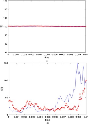
Table 1. Errors between real solution and simulated solution when $\alpha =1.2$.

	N = 100	N = 1000	N = 2000	N = 4000
Ture result	99.4476	99.3144	101.1549	96.6869
Simulation result	100.2488	99.3220	98.8646	96.6869
Error	0.8012	0.0076	2.2902	100.2224
Elapsed time	0.8390s	11.6680s	39.2940s	192.7890s

Table 2. Errors between real solution and simulated solution when $\alpha =1.4$.

Ture result	99.5066	99.3884	101.0203	97.0525
Simulation result	100.2206	99.3992	98.9940	100.2010
Error	0.7140	0.0109	2.0263	3.1485
Elapsed time	0.8300s	11.5600s	43.5960s	165.8050s

Table 3. Errors between real solution and simulated solution when $\alpha =1.6$.

Ture result	99.5517	99.4489	100.8662	97.4150
Simulation result	100.1915	99.4784	99.1268	100.1780
Error	0.6398	0.0295	1.7394	2.7630
Elapsed time	0.8700s	11.5390s	43.1650s	123.8970s

Table 4. Errors between real solution and simulated solution when $\alpha =1.8$.

Ture result	99.5905	99.5028	100.7108	97.7648
Simulation result	100.1630	99.5555	99.2561	100.1544
Error	0.5726	0.0527	1.4548	2.3896
Elapsed time	0.8380s	11.0380s	42.2730s	139.3090s

The table shows that the larger the coefficient N is, the better. Thus, a good error can be achieved when it is approximately 1000, and the time consumption is relatively small. The larger N makes the result worse and the longer the running time. To reduce error, we must optimize the algorithm, which is difficult to solve by modifying the coefficient. In literature [20], it is known that the model has only local weak convergence of order 1 and strong convergence of order $\frac{1}{2}$. This table shows that the choice of order has little effect on the experimental error results, and N has little effect on the error simulation of the model; thus, the model cannot improve the effect of the model by simply modifying the parameters. This result highlights an area for future work to be completed.

For the problem of solving stochastic equations, various disciplines are currently studying this problem and giving many research methods. For example, solve the nonlinear equation by linearizing it [21]; The R function method of Kudriahov, the Jacobian elliptic function method (JEFM) and the improved auxiliary equation method (MAE) are three effective and robust integration methods to help extract the solution of the equation [22]; Even scientists and researchers from different disciplines are dealing with fractional mixed boundary value problems [23]. The proofs of these studies in mathematical theory are excellent, but they are difficult to apply in real life. As can be seen from the table, this paper can find the solution of fractional order equation in a short time by using the backward method, which has certain computational advantages for the above methods, but the above methods are also very worthy of learning, The comparison of numerical experiments with various methods is also an important and interesting direction in the future.

7. Conclusion and future research

Because fractional ordinary differential equations can express the memory effect in the financial system, we establish a backward fractional stochastic differential equation through the fractional differential equation proposed by Tien [8]. At the same time, because the fractional differential equation can express the memory effect of the financial system when floating, we study the problem of integrating the stochastic process into the fractional differential equation, which can facilitate us to analyse the market volatility with memory. Therefore, after proving the existence and uniqueness of the solution, we also make a simple regression of the option price through fractional order stochastic differential equation. Because the memory indexes in the financial market typically, we only consider $H\in (0.5,1)$. Based on the fractional stochastic differential equation, we apply the method of constructing new norms to prove the Banach fixed point theorem and then obtain the existence and uniqueness of its solution. Finally, the comparison between the real solution and the simulated solution is given. It can be seen from the comparison chart that although the final simulation result after parameter adjustment can approximate the real solution, there are many errors in this method if it is the same as the real solution at all times. Based on the study of the existence and uniqueness of the solution of fractional stochastic differential equation, it can be found that if the stock price drift and volatility are driven by fractional order (that is, affected by the past state), it is also theoretically valid to inversely solve the option price according to the expectation at the last moment. Thus, if the neural network is used to solve the option pricing, it can also be used as the input of the neural network according to the past data, and the time length of this past data needs to be determined by continuous experiments. Of course, it will be particularly interesting to use different numerical methods to solve the numerical solution of the pricing of backward fractional stochastic differential options, which is also the main goal of the future work.

Disclosure statement

No potential conflict of interest was reported by the authors.

Additional information

Funding

The work was supported by the research grant from National Natural Science Foundation of China [grant number 62076039], Natural Science Foundation of Hubei Province [grant number 2022CFB023] and Commerce Statistical Society of China [grant number cssc-data21006].

References

- Hurst HE. Long-term storage capacity of reservoirs. Trans Am Soc Civ Eng. 1951;116(1):770–799.
- Garzarelli F, Cristelli M, Pompa G, et al. Memory effects in stock price dynamics: evidences of technical trading. Sci Rep. Mar 27, 2014;4:1–9.
- Hu Y, Peng S. Backward stochastic differential equation driven by fractional brownian motion. SIAM J Control Optim. 2009;48(3):1675–1700.
- Hussain S, Madi EN, Khan H, et al. On the stochastic modeling of COVID-19 under the environmental white noise. J Funct Sp. 2022;2022:1–9.
- Ahmad M, Zada A, Ghaderi M, et al. On the existence and stability of a neutral stochastic fractional differential system. Fractal Fract. 2022;6(4):203.
- Khan H, Alam K, Gulzar H, et al. A case study of fractal–fractional tuberculosis model in China: existence and stability theories along with numerical simulations. Math Comput Simul. 2022;198:455–473.
- Baleanu D, Jajarmi A, Mohammadi H, et al. A new study on the mathematical modelling of human liver with Caputo–Fabrizio fractional derivative. Chaos Solitons Fractals. 2020;134:Article ID 109705.
- Tien DN. Fractional stochastic differential equations with applications to finance. J Math Anal Appl. 2013;397(1):334–348.
- Wang J, Yan Y, Chen W, et al. Equity-linked securities option pricing by fractional brownian motion. Chaos Solitons Fractals. 2021;144:Article ID 110716.
- Caputo M. Linear models of dissipation whose q is almost frequency independent. Ann Geophys. 1966;19(4):383–393.
- Li Q, Zhou Y, Zhao X, et al. Fractional order stochastic differential equation with application in european option pricing. Discrete Dyn Nat Soc. 2014. DOI:10.1155/2014/621895
- McHiri L, Ben Makhlouf A, Baleanu D, et al. Finite-time stability of linear stochastic fractional-order systems with time delay. Adv Differ Equ. 2021;2021(1):1–10.
- Peng S. The backward stochastic differential equations and its application. Adv Math (NY). 1997;26(2):97–112.
- Ding D, Li X, Liu Y. A regression-based numerical scheme for backward stochastic differential equations. Comput Stat. 2017;32(4):1357–1373.
- Kuang J. Applied inequalities. Qingdao (China): Shandong Science and Technology Press; 2010.
- Liu P. Fundamentals of functional analysis. Beijing (China): Science Press; 2001.
- Klebaner FC. Introduction to stochastic calculus with applications. Singapore: World Scientific Publishing Company; 2012.
- Umamaheswari P, Balachandran K, Annapoorani N. Existence and stability results for Caputo fractional stochastic differential equations with Lévy noise. Filomat. 2020;34(5):1739–1751.
- Baghani O. On fractional langevin equation involving two fractional orders. Commun Nonlinear Sci Numer Simul. 2017;42:675–681.
- Urama TC, Ezepue PO. Stochastic ito-calculus and numerical approximations for asset price forecasting in the nigerian stock market. J Math Finance. 2018;8(04):640–667.
- Gençoğlu MT, Agarwal P. Use of quantum differential equations in sonic processes. Appl Math Nonlinear Sci. 2021;6(1):21–28.
- Arshed S, Raza N, Javid A, et al. Chiral solitons of (2+1)-dimensional stochastic chiral nonlinear schrödinger equation. Int J Geom Methods Mod Phys. 2022;19(10):2250149–3991.
- Aghili A. Complete solution for the time fractional diffusion problem with mixed boundary conditions by operational method. Appl Math Nonlinear Sci. 2021;6(1):9–20.