Application of constrained coefficient fuzzy linear programming in medical electrical impedance tomography

ABSTRACT

Electrical impedance tomography (EIT) is an imaging technique that realizes the image reconstruction of conductivity distribution in the field. The existing EIT algorithms ignore the hidden fuzzy features during imaging, making the EIT technique exhibit a high degree of uncertainty, imprecision, incompleteness, and inconsistency in the actual use process, resulting in a low spatial resolution of the reconstructed images. In order to solve this problem, we introduce fuzzy linear programming into EIT imaging. On the basis of analyzing the fuzzy features of EIT in detail, a new model of fuzzy optimization is built up, whose optimal solution is obtained by using constrained coefficient fuzzy linear programming. To this end, we devise two types of simulation experiments to verify the performance of the optimization algorithm. Experimental results prove that compared with the traditional Tikhonov regularization algorithm, the correlation coefficient of the reconstructed image of the proposed algorithm is higher, the relative error value is smaller.

KEYWORDS:

• Electrical impedance tomography
• fuzzy linear programming
• fuzzy features
• constraint coefficients
• image reconstruction
• uncertainty
• inverse problem
• Tikhonov regularization
• lung cancer detection
• model

MATHEMATICS SUBJECT CLASSIFICATIONS:

• 65N21
• 65J20
• 92C55

1. Introduction

Electrical impedance tomography (EIT), which first appeared in 1980s. It is a new generation of medical imaging technology developed in recent 40 years to obtain the resistivity or conductivity distribution of human internal tissues. This technology is based on the theory of electromagnetic field [1]. By placing the electrode on the surface of the human body and applying a safe excitation current, the voltage change of the corresponding electrodes are measured. And according to a certain image reconstruction algorithm, the distribution of the internal electrical features of the human body [2] is reconstructed to achieve functional imaging. Compared with traditional medical imaging techniques such as computed tomography [3] (CT), EIT has the advantages of safety and non-radiation, real-time non-destructive, fast response speed and low price. As a novel imaging technique, EIT has become a research hotspot of the majority of scholars in the medical field such as the early detection of lung diseases [4].

EIT has many advantages that traditional tomography technology does not have. However, due to the inherent ill-posedness and 'soft field' effects in the EIT process, coupled with the influence of various factors such as data signal-to-noise ratio, measurement conditions and operating conditions in the practical application process. Therefore, EIT shows high uncertainty, inaccuracy, incompleteness and inconsistency and other intrinsic properties in its use. These intrinsic properties limit the application areas of electrical impedance tomography, resulting in low spatial resolution of reconstructed image. Most research objectives cannot be clearly identified.

Over the past few decades, many EIT algorithms have been proposed by research scholars to overcome the above problems. Tikhonov regularity [5,6] (TR) is the most effective algorithm in most EIT processes. Using the rule term is beneficial to eliminate the effects of noise and obtain reconstructed images with higher spatial resolution. With the increasing requirements of spatial resolution of EIT imaging, iterative algorithms based on optimization theory have been successively applied to EIT problems. The most commonly used include Newton–Raphson algorithm [7], Landweber [8] iterative algorithm and so on. In recent years, Kalman filtering [9] and Sparse Bayesian Learning [10–12] are also applied to solve the EIT problem and achieved higher spatial resolution.

The existing EIT algorithms mainly rely on various mathematical optimization processes with deterministic objective functions and constraint equations, ignoring the hidden fuzzy features in the EIT imaging. It can neither effectively use the corresponding information of these fuzzy features, nor overcome the adverse effects of these features in the visualization process. Fuzzy set theory provides an effective tool for dealing with uncertain problems. The theory of fuzzy optimization is used to solve the EIT problem. The basic idea is to transform the fuzzy optimization problems into non-fuzzy optimization problems and obtain the optimal solution by various conventional algorithms. The focus of fuzzy optimization algorithms is to transform from fuzzy to non-fuzzy. Different transformation algorithms produce different fuzzy optimization solutions.

According to the previous research results of our group, we verify the feasibility of using fuzzy linear optimization model for EIT imaging reconstruction. The symmetric fuzzy linear programming algorithm [13] and the asymmetric fuzzy linear programming algorithm [14] based on fuzzy constraint information are applied to solve the inverse problem. Both algorithms obtain reconstructed image with higher spatial resolution on the discrete small target distribution [15]. Moreover, the results of previous studies have showed that adding prior information (known object contours, positions, etc.) to constraints can effectively improve the solution accuracy in some specific applications.

However, in previous studies, we ignored the effect of constraint coefficients on image reconstruction, and obtained the optimal solution by fuzzifying the constraint information. In the practical application of EIT, both the sensitivity coefficient matrix $\mathbf{\text{S}}$ and the boundary measurement value $\mathbf{\text{U}}$ are inaccurate, which is bound to have some effect on the reconstructed image quality. Moreover, in the previous study, we used circular field as the imaging field, which has a large model error compared with the actual thorax measurement field of the human body. The complex dynamic measurement environment of the human body greatly affects the accuracy of EIT imaging. Therefore, in order to further study the effectiveness of EIT algorithm based on fuzzy linear programming in the process of lung image reconstruction. Based on the detailed analysis of the inherent uncertain and fuzzy features of EIT process, we propose a fuzzy optimization algorithm based on constraint coefficient by using the fuzzy set theory and its expression form of membership degree. The sensitivity coefficient matrix $\mathbf{\text{S}}$ and boundary measurement value $\mathbf{\text{U}}$ are expressed by fuzzy membership degrees. The optimal solution of the proposed algorithm can be obtained by solving the fuzzy linear programming model. And simulation experiments are performed to verify that the model can more effectively improve the spatial resolution of the reconstructed images.

This paper is organized as follows. The second part briefly reviews the basic principles of EIT and the relevant theoretical knowledge of fuzzy linear programming. In the third part, the fuzzy features existing in the EIT process are analyzed in detail, and the fuzzy linear optimization model of EIT and its solution algorithm are established. The fourth part evaluates the effectiveness and feasibility of the proposed algorithm through a series of simulation experiments. The fifth part is conclusion.

2. Preliminaries

This section includes the basic principles of EIT and an introduction to the basic theory of fuzzy optimization.

2.1. Basic principles of EIT

A complete EIT system mainly includes three parts: sensor electrode array, data acquisition system and image reconstruction system, as shown in Figure 1.

Figure 1. Overall structure diagram of EIT system.

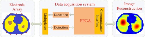
All boundary measurements can be collected by sequentially applying voltage or current signal excitations to the sensor electrode array. The data acquisition system filters, amplifies, modulates and demodulates the collected electrical signals, and sends them to the computer. The computer visualizes the conductivity distribution of the measured field in the form of a two-dimensional or three-dimensional image according to the received signal and combined with the image reconstruction algorithm.

The EIT process follows Maxwell's electromagnetic field theory [16] and follows the physical equations below: (1) $\mathrm{\nabla }\cdot (\sigma \cdot \mathrm{\nabla }\mathit{U})=0$(1) where$\sigma$is the conductivity; $\mathit{U}$is the potential distribution in the studied field.

In order to simplify the solution, the following assumptions can be made when appropriate: (1) Assuming that the sensitive field of EIT is quasi-stable field, a low-frequency constant current is injected on the surface of the imaging object, ignoring the displacement current; (2) The conductivity in the target imaging area is assumed to be scalar; (3) Ignore the three-dimensional effect of the current field and simplify it to a two-dimensional field; (4) The area measured by the actual electrode is not considered.

Based on the above assumptions, the mathematical model of EIT is expressed as (2) $\mathit{U}=\mathit{S}\mathit{g}$(2) where $\mathit{U}\in {\mathit{R}}^m$is the boundary measurement voltage vector; $\mathit{g}\in {\mathit{R}}^n$is the grey level vector; and $\mathit{C}\in {\mathit{R}}^n$ is the sensitivity coefficient matrix, which can be calculated in advance by the positive problem of EIT.

The EIT image reconstruction problem is to solve the conductivity distribution in the research field according to the boundary measurement data and the reference field sensitivity coefficient matrix. Finally, all the information of the spatial distribution of the substance in the measured area is expressed in the form of image grey value.

2.2. Fuzzy linear programming

Fuzzy linear programming [17] (FLP) is a generalization of classical linear programming. It can effectively show the imprecise and incomplete features which hidden in various measurements, and is widely used in image filtering, image enhancement, image fusion and other fields. FLP is a linear programming model based on the following criteria: (3) $minz=\mathbf{\text{C}}Xs.t.\mathbf{\text{A}}X\le \mathbf{\text{b}},\mathbf{\text{X}}\ge 0$(3) where, $\mathit{X}\in {\mathit{R}}^n$represents the decision variable; $z=\mathit{C}\mathit{X}$is the optimized objective function; $\mathit{A}\in {\mathit{R}}^{m\times n}$, $\mathit{b}\in {\mathit{R}}^m$, $\mathit{C}\in {\mathit{R}}^n$ represents the resource constraint matrix, resource possession vector and coefficient vector, respectively. When these conditions inherently have fuzzy features, they can be represented by fuzzy membership functions. Thus Equation (3)(3) $minz=\mathbf{\text{C}}Xs.t.\mathbf{\text{A}}X\le \mathbf{\text{b}},\mathbf{\text{X}}\ge 0$(3) is transformed into a fuzzy linear optimization problem.

Obviously, any part in Equation (3)(3) $minz=\mathbf{\text{C}}Xs.t.\mathbf{\text{A}}X\le \mathbf{\text{b}},\mathbf{\text{X}}\ge 0$(3) can be fuzzified in an appropriate way. For example, the constraint coefficient can be fuzzy number, the constraint condition can be written as fuzzy set, and the objective function can also be expressed as fuzzy set or fuzzy function. Selecting different fuzzy objects and fuzzy modes can lead to different types of fuzzy linear programming problems, mainly including the following types:

1. Linear programming model with fuzzy constraint coefficients. Such problems can be represented by the following model (4) $minz=\mathbf{\text{C}}Xs.t.\widetilde{\mathbf{\text{A}}}X\le \widetilde{\mathbf{\text{b}}},\mathbf{\text{X}}\ge 0$(4) where all or part of the elements of $\widetilde{\mathbf{\text{A}}}$,$\widetilde{\mathbf{\text{b}}}$ are fuzzy numbers.

2. Linear programming model with fuzzy constraints. The objective function is clear and the constraints are fuzzy. Such problems can be formulated as (5) $minz=\mathbf{\text{C}}Xs.t.\mathbf{\text{A}}X\tilde{\le }\mathbf{\text{b}},\mathbf{\text{X}}\ge 0$(5) where $\tilde{\le }$ denotes the fuzzy representation of the constraint condition with fuzzy membership relationship.

3. Linear programming model with fuzzy objective function. The objective function z is not required to reach the minimum value. It is only required to reach a certain level. That is, the optimality of the decision is replaced by the satisfaction of the decision. Such problems can be formulated as (6) $minz=\widetilde{\mathbf{\text{C}}}Xs.t.\mathbf{\text{A}}X\le \mathbf{\text{b}},\mathbf{\text{X}}\ge 0$(6)

3. Fuzzy optimal solution of the EIT process

In this section, the hidden fuzzy features in the EIT image reconstruction process are analysed. We established the fuzzy model of EIT process, and obtained the optimal solution by the FLP algorithm, in order to improve the image spatial resolution of EIT.

3.1. Fuzzy features in EIT

The fuzzy features of the EIT process are analysed from the following aspects.

3.1.1. Uncertainty of the sensitive coefficient matrix

In the EIT system, the uncertainty of the sensitive coefficient matrix [18] is mainly reflected in the following two aspects.

1. Non-additivity of sensitivity coefficient matrix

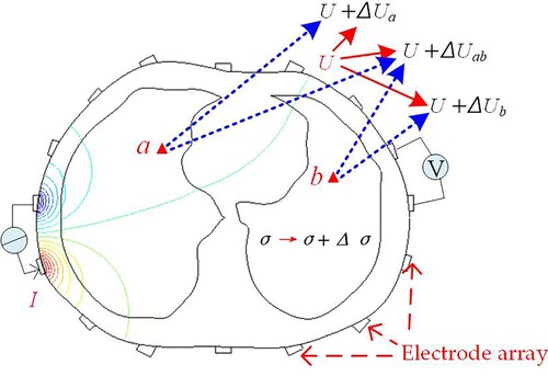
The two red triangles in Figure 2 represent the pixels $a$ and $b$, respectively. When pixel $a$ and $b$ respectively increase a unit of conductivity (from $\sigma$ to $\sigma +\mathrm{\Delta }\sigma$), the voltage variation of a pair of measuring electrodes is $\Delta U_a$ and $\Delta U_b$. When pixel $a$ and $b$simultaneously increase a unit of conductivity, the voltage variation of the measuring electrodes is $\Delta U_{ab}$. Due to the presence of soft field effect in the EIT system, the change of conductivity of each pixel affects the measurement data of all the adjacent electrodes. This results in that the additivity is not satisfied between the three voltage changes mentioned above, namely: $\Delta U_{ab}\ne \Delta U_a+\Delta U_b$.

1. Uncertainty of 'empty field' sensitivity coefficient matrix

Figure 2. Effect of pixel conductivity change on boundary measurements.

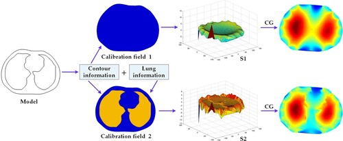
'Empty field' is a hypothetical uniform field. 'Full field' refers to the object field corresponding to the actual target. The distribution of objects within the field domain will affect the distribution of the electric field, which leads to changes in the sensitivity matrix. The sensitivity coefficient matrix obtained according to 'empty field' and 'full field', respectively, are very different. In the reconstruction model $U=Sg$, $S$ should be the sensitivity coefficient matrix of 'full field' (corresponding to the real distribution). It is obvious that the conductivity distribution of 'full field' is unknown, and the corresponding sensitivity coefficient matrix is not available. Therefore, in the dynamic imaging algorithm based on sensitivity coefficient matrix, we consider the medium distribution in the sensitive field to be approximately unchanged when it is assumed that the conductivity distribution changes little. We can build the model in COMSOL at a 1:1 ratio according to the physical size of the real sensitive field and the electrode size. We can obtain the 'empty field' sensitivity coefficient matrix by solving the positive problem, and assume that the 'empty field' and 'full field' obey the same sensitivity coefficient matrix. Then the 'empty field' sensitivity coefficient matrix is directly used for image reconstruction. Since the sensitivity coefficient matrix of 'full field' is not equal to the value of empty field, this causes inaccuracy of reconstruction results.

Figure 3 shows a comparison of the 'empty field' sensitivity coefficient matrix and the 'full field' sensitivity coefficient matrix. The first row shows the distribution of 'empty field' sensitivity and the second row shows the distribution of 'full field' sensitivity. From the simulation results, it can be seen that the 'empty field' sensitivity coefficient matrix and the 'full field' sensitivity coefficient matrix are quite different, especially from the perspective of the sum of sensitivity. The full field sensitivity coefficient matrix completely contains the target information, including the location and shape of the target. The reconstructed images obtained by using the conjugate gradient (CG) algorithm [19] are based on the 'empty field' and 'full field' sensitivity coefficient matrices, respectively, as shown in the last column of Figure 3. It can be seen that the model can be identified by using the 'full field' sensitivity coefficient matrix, while the target is basically unidentifiable by using the 'empty field' sensitivity coefficient matrix.

Figure 3. Comparison of sensitivity coefficients between empty field and full field.

3.1.2. Inaccuracy of measurement data

Lungs are not regular shapes, which making imaging difficult. EIT does not provide precise anatomical localization of the tissue. The closer to the centre of the body, the greater the influence of various biological tissues, resulting in lower spatial resolution. The 'soft field' effect during EIT means that any boundary measurement data is associated with all rather than part of the pixels in the field. That is, a subtle change in the conductivity of any target within the field will cause a change in the measurements of all electrodes at the field boundary. However, due to the complex dynamic measurement environment of the human body, the imaging accuracy of EIT technology in the medical field is greatly affected. Sometimes small measurement changes caused by lesions may not be too obvious on the reconstructed images. Therefore, this measurement mechanism of EIT makes the boundary measurement more unreliable and inaccurate, which has a great impact on the application of electrical impedance imaging technology in the field of medical research.

3.1.3. Diversity of parameters in the objective function

In the reconstruction algorithms based on regularization algorithm, the selection of regularization parameters has a great impact on the spatial resolution of the reconstructed image. Table 1 shows a set of images reconstructed by the Tikhonov regularization algorithm. The first column is the original image, and 2∼5 columns correspond to the reconstructed images with different regularization parameters λ and the correlation coefficient (CC).

Table 1. Correlation coefficient and regularization parameters of reconstructed images by Tikhonov regularization algorithm.

λ	0.2	0.0002	0.000002	0.00000000002
CC	0.1255	0.3467	0.4230	0.4289
λ	0.0002	0.000002	0.00000002	0.00000000002
CC	0.1749	0.4534	0.6457	0.2942

It can be seen from the reconstructed image that the spatial resolution of the reconstructed image is quite different under different regularization parameters, and the corresponding correlation coefficient values are also different. In the first model with only one pathological target, when the regularization parameter is $2\times {10}^{\text{ - }11}$, the reconstructed image has the best quality and the correlation coefficient CC value is the highest. In the second model, when the regularization parameter is $2\times {10}^{\text{ - }8}$, the reconstructed image has the best effect and the correlation coefficient CC value is the highest. It can be seen that the regularization parameters of the corresponding optimal spatial resolution are different under the two different models, which hinders the application of the algorithm. Although many scholars have studied the selection of regularization parameters and proposed different algorithms to obtain their optimal values. However, there is no doubt that the uncertainty of regularization parameters is still a bottleneck affecting the application of regularization algorithms.

3.2. Constrained coefficient fuzzy linear programming model with its algorithm

In summary, in EIT image reconstruction, the fuzzy features are mainly reflected in the inaccuracy of sensitivity coefficient matrix and measured values. Combined with the mathematical model of Equation (2)(2) $\mathit{U}=\mathit{S}\mathit{g}$(2) . The basic parameter variables are fuzzified and solved by the algorithm of constrained coefficient fuzzy linear programming.

According to the fuzzy set theory and the membership degree representation form, a fuzzy linear programming model with constraint coefficients (CCFLP) is established which can be expressed as: (7) $minz=\mathbf{\text{C}}g,s.t.\begin{array}{c}\widetilde{\mathbf{\text{S}}}g\le \widetilde{\mathbf{\text{U}}},\mathbf{\text{g}}\ge 0\end{array}$(7) where $\mathit{g}\in {\mathbf{\text{R}}}^n$ denotes the decision variable, i.e. the image grey level vector; $z=\mathit{C}\mathit{g}$ is the optimized objective function; $\tilde{\mathit{S}}\in {\mathit{R}}^{m\times n}$,$\tilde{\mathit{U}}\in {\mathit{R}}^m$,$\mathit{C}\in {\mathit{R}}^n$represent the importance of the sensitivity coefficient matrix, boundary measure vector, and pixel, respectively.

Assuming that the elements ${\tilde{\mathit{S}}}_{ij}$, ${\tilde{\mathit{U}}}_i$, $i=1,2,\cdots ,m$, $j=1,2,\cdots ,n$ in $\widetilde{\mathbf{\text{S}}}$, $\widetilde{\mathbf{\text{U}}}$ all satisfy the trapezoidal fuzzy number, i.e. ${\tilde{\mathit{S}}}_{ij}=\left(m_{ij},n_{ij},{\alpha }_{ij},{\text{β}}_{ij}\right)$, ${\tilde{\mathit{U}}}_i=\left(p_i,q_i,{\gamma }_i,{\delta }_i\right)$. It can be seen from the operational properties of the trapezoidal fuzzy number:

$\mathrm{\forall }{g}_j,j=1,2,\cdots ,n$, $\sum _{j=1}^n{\tilde{\mathit{S}}}_{ij}{\mathit{g}}_j$ are also trapezoidal fuzzy numbers and have: (8) $\sum _{j=1}^n{\tilde{\mathit{S}}}_{ij}{\mathit{g}}_j=\left(\sum _{j=1}^n{m}_{ij}{g}_j,\sum _{j=1}^n{n}_{ij}{g}_j,\sum _{j=1}^n{\alpha }_{ij}{g}_j,\sum _{j=1}^n{\text{β}}_{ij}{g}_j\right)$(8)

Thus, the constraint condition in model (7) can be expressed as (9) $\begin{array}{c}(\sum _{j=1}^n{m}_{ij}{g}_j,\sum _{j=1}^n{n}_{ij}{g}_j,\sum _{j=1}^n{\alpha }_{ij}{g}_j,\sum _{j=1}^n{\text{β}}_{ij}{g}_j)\le (p_i,q_i,{\gamma }_i,{\delta }_i)\end{array}$(9) So, model (7) is transformed into: (10) $\begin{array}{l}minz=\mathbf{\text{C}}g,\begin{array}{c}\end{array}\\ s.t.\begin{array}{r}\end{array}\begin{array}{c}(\sum _{j=1}^n{m}_{ij}{g}_j,\sum _{j=1}^n{n}_{ij}{g}_j,\sum _{j=1}^n{\alpha }_{ij}{g}_j,\sum _{j=1}^n{\text{β}}_{ij}{g}_j)\le (p_i,q_i,{\gamma }_i,{\delta }_i),\mathbf{\text{g}}\ge 0\end{array}\end{array}$(10)

According to the ranking criterion of fuzzy numbers, the above constraints are equivalent to: (11) $\{\begin{array}{l}\sum _{j=1}^n{m}_{ij}{g}_j\le p_i\\ \sum _{j=1}^n(m_{ij}-{\alpha }_{ij})g_j\le p_i-{\gamma }_i\\ \sum _{j=1}^n{n}_{ij}{g}_j\le q_i\\ \sum _{j=1}^n(n_{ij}+{\text{β}}_{ij})g_j\le q_i+{\delta }_i\end{array}$(11) Therefore, the solution model (10) can be transformed into the following ordinary mathematical programming: (12) $\begin{array}{l}minz=\mathbf{\text{C}}g,\begin{array}{c}\end{array}\\ \begin{array}{c}s.t.\begin{array}{r}\end{array}\{\begin{array}{l}\sum _{j=1}^n{m}_{ij}{g}_j\le p_i,\begin{array}{r}\end{array}\sum _{j=1}^n(m_{ij}-{\alpha }_{ij})g_j\le p_i-{\gamma }_i\\ \sum _{j=1}^n{n}_{ij}{g}_j\le q_i,\begin{array}{r}\end{array}\sum _{j=1}^n(n_{ij}+{\text{β}}_{ij})g_j\le q_i+{\delta }_i\\ \mathbf{\text{g}}\ge 0\end{array}\end{array}\end{array}$(12)

The optimal solution of the fuzzy optimization model (7) can be obtained by solving the linear programming (12). Table 2 lists the CCFLP algorithm in the EIT process.

Table 2. CCFLP algorithm implementation steps.

Input: Boundary measure $\mathbf{\text{U}}$, Sensitivity coefficient matrix $\mathbf{\text{S}}$
Output: Gray level vector $\mathbf{\text{g}}$
Step: 1. Establish the model (7) according to the fuzzy set theory and membership degree representation form;
2. Obtain constraint (9) according to equation (8)(8) $\sum _{j=1}^n{\tilde{\mathit{S}}}_{ij}{\mathit{g}}_j=\left(\sum _{j=1}^n{m}_{ij}{g}_j,\sum _{j=1}^n{n}_{ij}{g}_j,\sum _{j=1}^n{\alpha }_{ij}{g}_j,\sum _{j=1}^n{\text{β}}_{ij}{g}_j\right)$(8) , and then equate equation (7)(7) $minz=\mathbf{\text{C}}g,s.t.\begin{array}{c}\widetilde{\mathbf{\text{S}}}g\le \widetilde{\mathbf{\text{U}}},\mathbf{\text{g}}\ge 0\end{array}$(7) with equation (10)(10) $\begin{array}{l}minz=\mathbf{\text{C}}g,\begin{array}{c}\end{array}\\ s.t.\begin{array}{r}\end{array}\begin{array}{c}(\sum _{j=1}^n{m}_{ij}{g}_j,\sum _{j=1}^n{n}_{ij}{g}_j,\sum _{j=1}^n{\alpha }_{ij}{g}_j,\sum _{j=1}^n{\text{β}}_{ij}{g}_j)\le (p_i,q_i,{\gamma }_i,{\delta }_i),\mathbf{\text{g}}\ge 0\end{array}\end{array}$(10) ;
3. According to the ranking criterion of fuzzy number, the constraint condition of formula (10) is equivalent to (11), and then formula (12) is obtained;
4. Obtain equation (12)(12) $\begin{array}{l}minz=\mathbf{\text{C}}g,\begin{array}{c}\end{array}\\ \begin{array}{c}s.t.\begin{array}{r}\end{array}\{\begin{array}{l}\sum _{j=1}^n{m}_{ij}{g}_j\le p_i,\begin{array}{r}\end{array}\sum _{j=1}^n(m_{ij}-{\alpha }_{ij})g_j\le p_i-{\gamma }_i\\ \sum _{j=1}^n{n}_{ij}{g}_j\le q_i,\begin{array}{r}\end{array}\sum _{j=1}^n(n_{ij}+{\text{β}}_{ij})g_j\le q_i+{\delta }_i\\ \mathbf{\text{g}}\ge 0\end{array}\end{array}\end{array}$(12) and obtain the optimal solution.

4. Experiments

To verify the performance of the CCFLP optimization algorithm, we carry out two types of simulation studies. One is to use the CCFLP algorithm to reconstruct the images of four typical lung cancer models. The other is to select the small cell cancer model from four typical lung cancer models for conductivity sensitivity test. Among them, the second experiment is to verify whether the CCFLP algorithm can reconstruct the image target earlier and more accurately under different conductivity conditions.

In the simulation, the finite element algorithm based on triangular adaptive mesh is used to solve the positive problem and calculate the sensitivity coefficient matrix. In the inverse problem solving, the measured field is divided into a grid of 1290 square elements to reconstruct the conductivity distribution. Sixteen electrodes are used in the thoracic field. And the number of measured voltages is 208 according to the mode of adjacent excitation and adjacent measurement.

Simulation conditions: running on Intel (R) i5 3.2 GHz CPU, 4 GB memory PC. Development platform version: COMSOL3.5, MATLAB2012.

4.1. Image quality evaluation indicators

Different evaluation indexes are used to evaluate the spatial resolution of reconstructed images. Commonly used supervision and evaluation indicators are:

1. Correlation coefficient [20] (CC). The CC reflects the degree of similarity between the reconstructed image and the reference image. The larger value of the correlation coefficient, the higher spatial resolution of the reconstructed image. The correlation coefficient is defined as: (13) $CC=\frac{{\sum }_{i=1}^N({\mathbf{\text{g}}}_i-\overline{\mathbf{\text{g}}})({\mathbf{\text{g}}}_i^{\ast }-{\overline{\mathbf{\text{g}}}}^{\ast })}{\{{\sum }_{i=1}^N{({\mathbf{\text{g}}}_i-\overline{\mathbf{\text{g}}})}^2{\sum }_{i=1}^N{({\mathbf{\text{g}}}_i^{\ast }-{\overline{\mathbf{\text{g}}}}^{\ast })}^2{\}}^{1/2}}$(13) where, $\mathbf{\text{g}}$represents the conductivity calculated by the image reconstruction algorithm; ${\mathbf{\text{g}}}^{\ast }$ represents the conductivity actually distributed in the field. ${\mathbf{\text{g}}}_i$ and ${\mathbf{\text{g}}}_i^{\ast }$are the $i$ th element of $\mathbf{\text{g}}$ and ${\mathbf{\text{g}}}^{\ast }$; $\overline{\mathbf{\text{g}}}$ and $\overline{\mathbf{\text{g}}}\ast$ are the mean values of $\mathbf{\text{g}}$and ${\mathbf{\text{g}}}^{\ast }$, respectively. N represents the number of pixels divided. From the above equation, it can be seen that the larger the value of $\alpha$, the stronger the correlation between the reconstructed image and the set model, that is, the accuracy of the reconstructed image.

2. Relative error [20] (RE). RE denotes the error between the reconstructed image and the reference image. The smaller the relative error, the higher spatial resolution of the reconstructed image. The relative error is defined as: (14) $RE=\frac{||\mathbf{\text{g}}-{\mathbf{\text{g}}}^{\ast }||}{||{\mathbf{\text{g}}}^{\ast }||}$(14) where$\mathbf{\text{g}}$is the real electrical characteristic parameter distribution and${\mathbf{\text{g}}}^{\ast }$is the reconstructed electrical characteristic parameter distribution.

4.2. Simulation of different types of lung cancer cell models

In order to verify the performance of the CCFLP optimization algorithm, we established four typical lung cancer (squamous cell carcinoma, adenocarcinoma, large cell carcinoma, small cell carcinoma) models according to the distribution of different lung cancer cells for simulation study. Among them, most of the adenocarcinomas are located in the periphery of the lung, with consistent cell size. Squamous cell carcinomas often occupy the centre of the lung, which is a central lung cancer with no hierarchy. Small cell carcinomas are located in the centre of the lung, with consistent size, and cytological specimens show syncytial-like cell clusters or single tumour cells arranged in a linear pattern. And large cell carcinomas are often arranged in a palisade pattern.

COMSOL 3.5 is used for modelling. Adjacent current excitation are used and boundary measurements are calculated by finite element profile simulation. Set thoracic conductivity to 1, two lungs conductivity to 2 and lesion target conductivity to 3. Based on the same measurement value, Tikhonov regularization algorithm is selected for comparison reference. The regularization parameter is selected 2 × 10⁻⁵ according to the empirical value. The simulation experimental results are shown in Figure 4.

Figure 4. Reconstructed images of four lung cancer models.

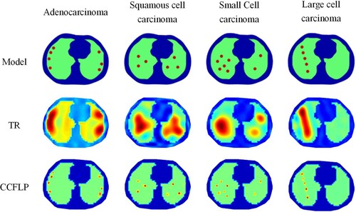
As shown in Figure 4, there are three rows of images. Among them, the first row of images is the simulation model established for four typical types of lung cancer, which is followed by adenocarcinoma, squamous cell carcinoma, small cell carcinoma and large cell carcinoma from left to right. The second row of images is the reconstruction images of Tikhonov regularization algorithm. And the third row of images is the images reconstructed by the constraint coefficient fuzzy optimization algorithm proposed in this paper. From the simulation results, it can be seen that the TR algorithm can not accurately find all the targets, and the false track is large. Closer targets are mixed together, and the target boundary is blurred, making it impossible to clearly see the location and number of targets. Compared with TR algorithm, CCFLP algorithm has higher spatial resolution. The background of the reconstructed image is clear. And the target boundary artifacts are less. Especially for small targets with discrete arrangement distribution in adenocarcinoma and large cell carcinoma, the location, number and boundary contour of targets can be clearly presented.

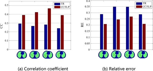
The above reconstructed image results are further quantified using the correlation coefficient CC and the relative error RE, and are expressed in the form of histograms, as shown in Figure 5. It can be seen from the results that compared with the traditional Tikhonov regularization algorithm, the CC value of the reconstructed image obtained by the CCFLP algorithm is increased by 55.06% on average, and the RE value is decreased by 27.03% on average. It indicates that the CCFLP algorithm can more effectively improve the spatial resolution of the EIT reconstructed image.

Figure 5. Image quality evaluation indicators of four lung cancer models. (a) Correlation coefficient and (b) Relative error.

4.3. Sensitivity test for conductivity

According to the development mechanism of molecular pathology, the course of lung tissue development from normal to cancerous is a gradually changing process. Previous studies by our group have also shown that the lesion process of lung cancer tissues is positively correlated with tissue conductivity [21]. That is, when lung tissues become cancerous, their conductivity usually increases [22].

In order to verify the sensitivity of the CCFLP algorithm to changes in conductivity, we select small cell carcinoma models from four typical lung cancer models for conductivity sensitivity testing. We simulate earlier diseased tissues by changing the conductivity of certain pixel blocks (red markers) in the lungs. The conductivity change increment is $\Delta \sigma$. Based on the same measurement value, TR algorithm is used for comparison. And the regularization parameter is set to 2 × 10^{− 5} based on empirical values. The simulation results are shown in Figure 6.

Figure 6. Reconstruction results at different values of $\Delta \sigma$ in the lesion part of small cell carcinoma model.

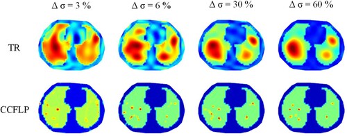
As shown in Figure 6, the first row is the conductivity change increment. The second row is the reconstructed image of Tikhonov regularization algorithm. The third row is the reconstructed image of constraint coefficient fuzzy optimization algorithm. In Figure 6, it can be seen that no matter how much the conductivity of the lesion target increases, the spatial resolution of the reconstructed image of the CCFLP algorithm is higher than that of the traditional TR algorithm. In the left lung of the model, there are many and densely distributed lesion targets. The TR algorithm cannot reconstruct the number, size and location of targets, but can generally present the outline of all targets. The CCFLP algorithm can identify the location of small targets and present individual targets one by one. Especially when $\Delta \sigma \text{ = 60\%}$, the CCFLP algorithm can accurately reconstruct the location and size of all small targets. However, when $\Delta \sigma \le 30\text{\%}$, the number of reconstructed targets is slightly biased. The simulation results show that the CCFLP algorithm has higher image spatial resolution than the TR algorithm. And it can reconstruct the location, size and number of lesion targets earlier and more accurately. Therefore, the CCFLP algorithm can be used in the early detection of pulmonary diseases.

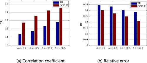
The above reconstructed image effect can be further quantified by the correlation coefficient and relative error, as shown in Figure 7. From the results, it can be seen that the correlation coefficient is increasing and the relative error is decreasing as the target conductivity is increasing. Moreover, the reconstructed images obtained by the CCFLP algorithm had larger CC values and smaller RE values compared with the reconstructed images by the TR algorithm.

Figure 7. Image quality evaluation indicators at different values for the lesion part of small cell carcinoma. (a) Correlation coefficient and (b) Relative error.

5. Conclusion

In order to solve the problem of low spatial resolution in the process of EIT image reconstruction, we have analyzed the implicit fuzzy features in the EIT process in detail and have revealed that fuzzy features is an essential attribute of the EIT process: uncertainty, imprecision, incompleteness, and inconsistency. However, the existing EIT algorithms can neither effectively utilize the corresponding information of these fuzzy features, nor overcome the adverse effects of these features in the visualization process. Therefore, in this paper, we have established a constrained coefficient fuzzy linear programming model to obtain the optimal solution. Based on the proposed optimization algorithm, we have carried out two types of simulation experiments for different lung cancer cell models. And the reconstruction results have shown that the CCFLP algorithm has higher spatial resolution of the reconstructed image, more accurate location, size and number of lesion targets, higher correlation coefficient values, and smaller relative error values than the traditional TR algorithm. Moreover, the experimental results of conductivity sensitivity test have shown that the CCFLP algorithm can detect the lesion target earlier and more accurately than the TR algorithm. Therefore, the CCFLP optimization algorithm has high practicability and superiority in medical fields such as early detection of pulmonary diseases.

Disclosure statement

No potential conflict of interest was reported by the author(s).

Additional information

Funding

This research was funded by the National Science Foundations of China [grant number 61973 232] and the Natural Science Foundation of Shandong Province [grant number ZR2021MF083].

References

- Feng CZ, Ma XK. An introduction to engineering electromagnetic fields. Beijing: Higher Education Press; 2000.
- Watson FM, Grabb MG, Lionheart WRB. A polarization tensor approximation for the Hessian in iterative solvers for non-linear inverse problems. Inverse Probl Sci Eng. 2021;29(13):2804–2830.
- Fathalla KM, Youssef SM, Mohammed N. DETECT-LC: A 3D deep learning and textural radiomics computational model for lung cancer staging and tumor phenotyping based on computed tomography volumes. Applied Sciences. 2022;12(13):6318.
- Manika J, Richa G, Rajiv, S. A Review on Non-Invasive Biosensors for Early Detection of Lung Cancer. 2020 6th International Conference on Signal Processing and Communication (ICSC). 2020:162-166.
- Wang J. Non-convex ℓp regularization for sparse reconstruction of electrical impedance tomography. Inverse Probl Sci Eng. 2021;29(7):1032–1053.
- Li X, Yang F, Yu X, et al. Study on the inverse problem of electrical impedance tomography based on self-diagnosis regularization. J Biomed Eng. 2018;35(3):460–467.
- Hu HL, Liu X, Wang XX, et al. A self-adapting Landweber algorithm for the inverse problem of electrical capacitance tomography (ECT). Instrumentation and Measurement Technology Conference Proceedings (I2MTC). 2016: 1–6.
- Wang J, Bo H. Application of a class of iterative algorithms and their accelerations to Jacobian-based linearized EIT image reconstruction. Inverse Probl Sci Eng. 2021;29(8):1108–1126.
- Zhang LF, Liu ZL, Tian P. Image reconstruction algorithm for electrical capacitance tomography based on compressed sensing. Acta Electron Sin. 2017;45(2):353–358.
- Liu SH, Huang YM, Wu HC, et al. Efficient multitask structure-aware sparse Bayesian learning for frequency-difference electrical impedance tomography. IEEE Trans Ind Inf. 2021;17(1):463–472.
- Liu SH, Cao RS, Huang YM, et al. Time sequence learning for electrical impedance tomography using Bayesian spatiotemporal priors. IEEE Trans Instrum Meas. 2020;69(9):6045–6057.
- Liu SH, Wu HC, Huang YM, et al. Accelerated structure-aware sparse Bayesian learning for three-dimensional electrical impedance tomography. IEEE Trans Ind Inf. 2019;15(9):5033–5041.
- Ding ML, Yue SH, Song K, et al. Fuzzy optimal solution of electric tomography imaging: modelling and application. Flow Meas Instrum. 2018;59:72–78.
- Ding ML, Yue SH, Li J, et al. Application of asymmetric fuzzy linear programming in EIT. 2019 IEEE international instrumentation and measurement technology conference(I2MTC), Auckland, New Zealand. 2019:1–5.
- Chien-Hsin T, Ko-Han L, Chuang-Hsin C, et al. Simultaneous time-of-flight PET/MR identifies the hepatic 90Y-resin distribution after radioembolization. Clin Nucl Med. 2020;45(2):e92–e93.
- Mazur O, Awrejcewicz J. Ritz method in vibration analysis for embedded single-layered graphene sheets subjected to In-plane magnetic field. Symmetry (Basel). 2020;12(4):515.
- Zhou XH, Jia HX, Huang XH, et al. Model and algorithm of the bi-level multiple followers linear programming with trapezoidal fuzzy decision variables[J]. Chinese Journal of Engineering Mathematics. 2021;38(01):49–62.
- Li J, Yue SH, Wang YR. Electrical impedance tomography of human lung canceer based on prior information[J]. Transducer and Microsystem Technologies. 2018;37(10):22–24.
- Bala AA, Maulana M, Poom K, et al. A liu-storey-type conjugate gradient algorithm for unconstrained optimization with application in motion control[J]. Journal of King Saud University Science. 2022;34(4):146–157.
- Fan WR, Mo XF. Electrical impedance tomography based on improved L1/2 regularization[J]. Electronic Measurement Technology. 2022;45(07):56–61.
- Wang YR. Study on auxiliary detection methods of lung cancer and air pollution factors affecting lung cancer[D]. Tianjin University, 2019.
- Sun X, Lee E, Choi J. Quantification of measurement error effects on conductivity reconstruction in electrical impedance tomography. Inverse Probl Sci Eng. 2020;28(12):1669–1693.