Highly efficient numerical scheme for solving fuzzy system of linear and non-linear equations with application in differential equations

ABSTRACT

In this research, we suggested a numerical iterative scheme for investigating the numerical solution of fuzzy linear and nonlinear systems of equations, particularly where the linear or nonlinear system co-efficient is a crisp number and the right-hand side vector is a triangular fuzzy number. Triangular fuzzy systems of linear and nonlinear equations play a critical role in a variety of engineering, scientific challenges, mathematics, chemistry, physics, artificial intelligence, biology, medical, economics, finance, statistics, machine and deep learning, computer science, robotics and smart cars, programming, in the military and engineering industries, linear and nonlinear programming problems and traffic flow problems. In biomedical engineering, fluid flow problems, and differential equations, triangular fuzzy linear and nonlinear systems of equations also play a key role in determining the level of uncertainty. Convergence analysis illustrates that the proposed numerical technique's order of convergence for solving a triangular fuzzy system of linear and nonlinear equations is three. The newly developed numerical scheme was then applied to solve several triangular fuzzy boundary value problems. In terms of convergence rate, computing time, and residual error, numerical test problems indicate that the newly developed methods are more efficient than the current methods in the literature.

KEYWORDS:

• Numerical schemes
• triangular fuzzy number
• CPU-time
• order of convergence
• numerical solutions

SUBJECT CLASSIFICATION CODE:

• 08A72
• 34A34

Introduction

Numerous scientific, mathematical and engineering problems are simulated using real data, most of which are ambiguous, incorrect, or insufficient. In other words, detailed information regarding parameter values, functional relationships, or initial conditions is not provided. In these cases, the selected behaviour of the system can only be estimated using existing analytical or numerical techniques. For example, by changing the values of unknown parameters to more reliable ones. It is impossible to describe the behaviour of a whole system based on incomplete knowledge. Thus, in many dynamical models, a system of nonlinear equations occurs. Nonlinear systems of equations, rather than a single bit, are widely used to describe a wide range of real-world problems. The uncertainty in these types of linear or nonlinear systems of equations can be well represented by triangular fuzzy numbers, and such a system is known as a triangular fuzzy system of linear or nonlinear equations. Triangular fuzzy linear and nonlinear systems of equations are not often solved using analytical methods. As a result, because of their wider range of stability and consistency, we look to numerical iterative schemes.

The fuzzy set and fuzzy logic theories were initially put forward by Zadeh in a number of books and series of papers e.g. [1,2]. This improvement enables the extension of the crisp mathematical concept into fuzzy information. Theoretically, Dubois and Prade [3,4], Tanaka and Mizumoto [5,6], Chang et al. [7] and Nahmias [8] established the fundamental operations and studied fuzzy numbers techniques. Goetschel et al. [9] presented the parametric form of fuzzy numbers and the concept of fuzzy calculus. They went one step further and integrated the parametric fuzzy number set into a topological vector space. The concept of triangular fuzzy numbers was first introduced by Moghadam et al. [10]. Furthermore, Wu et al. [11] and Puri et al. [12] examined a variety of other useful literary ideas in reference to their previously published work. Both engineering and science frequently employ linear systems. When attempting to solve a problem, we estimate most of the time. Instead of using crisp numbers to convey a few parameters, several applications employ triangular fuzzy and broader fuzzy. Numerical techniques must be proposed in order to properly analyse and solve triangular fuzzy linear and nonlinear systems of equations (TFSNEs). Many fields of technology and engineering sciences, including telecommunications, statistics, economics, social sciences, image processing, and even physics, use parametric fuzzy numbers (PFNs) [13–15] to solve fuzzy systems of linear equations (FSLEs) with real crisp coefficient entries and vectors on the right-hand side. For more details on triangular fuzzy number (TFN) and their applications, see e.g. [16–23].

To approximate roots of fuzzy non-linear equations or system of nonlinear equations, Abbsbandy et al. [24] used Newton Raphson method, Ibrahim et al. [25] used Levenberg-Marquest Method, Mosleh et al. [26] used Adomian Decomposition Method, [27,28], modify existing iterative methods [29], used Levenberg-Marquardt method [30], used numerical techniques to solve fuzzy dynamic system see also [31,32]. The primary goal of this research is to suggest an efficient higher order iterative approach that outperforms well-known classical methods such as the Newton–Raphson method [6,33].

To develop and analyse higher order efficient numerical schemes for solving TFSNE, however, almost no work has been done. Consequently, there is a lot of potential for advancement and development in these areas. Since not much work has been done, we must establish the basic aspects and findings that are necessary for the proper development of this domain. Motivated by the aforesaid work, in this article, we have developed higher order numerical scheme to solve the TFSNEs and TFBVPs. In the future, this article may help other researcher with the further development of this topic.

The following are the article's main contributions:

• Define TFN and its arithmetic operations

• Use a parametric form of TFN in TFSNEs

• Proposed new numerical iterative scheme in Triangular fuzzy environment

• Compute theoretical convergence order of the proposed method using convergence analysis

• Numerical test examples are given to demonstrate the precision and accuracy of the suggested approach and the graphically shown result of the problem

• Some triangle fuzzy boundary value problems, both linear and nonlinear, are considered and solved

• The results of our proposed method are compared to those of existing methods

This article is divided into the following five sections. Section 2 goes through some basic concepts for triangular and trapezoidal fuzzy numbers. We propose and analyse a numerical iterative scheme for solving triangular fuzzy linear (TFSLEs) and triangular fuzzy nonlinear systems of equations in Section 3. Section 4 depicts some real-world applications as numerical test cases to demonstrate the performance and efficiency of the newly constructed method, with conclusions in the last section.

Preliminaries

Definition 1:

A fuzzy number is a fuzzy set like $x:\text{R}\to I=[0,1]$ which satisfies [34],

1. $x$ is upper semi-continuous,

2. $x\left(r\right)=0$ outside some interval$[e_1,e_2]$,

3. There are real numbers $a_1,a_2$such that ë $1\le a_1\le a_2\le e_2$ and

4. $x\left(r\right)$ is monotonic increasing on $\left[e_1,a_1\right]$,

5. $x\left(r\right)$ is monotonic decreasing on $\left[a_2,e_2\right]$,

6. $x\left(r\right)=1$, for $a_1\le e\le a_2$

We denote by $E,$ the set of all fuzzy numbers. An equivalent parametric form is also given in Ref. [35] as follows.

Definition 2:

[36] A fuzzy number $x$ in parametric form is a pair $\left(x^L,x^U\right)$ of function $x^L\left(r\right),$ $x^U\left(r\right),$ $0\le r\le 1,$ which satisfies the following requirements:

1. $x^L\left(r\right)$ is a monotonic increasing left continuous function that is bounded.

2. $x^U\left(r\right)$ is a monotonic decreasing left continuous function that is bounded.

3. $x^L\left(r\right)\le x^U\left(r\right),$ $0\le r\le 1.$

A popular fuzzy number is trapezoidal fuzzy number $A,$ denoted by $A=\left({\ddot{e}}_1,{\ddot{e}}_2,{\ddot{e}}_3,{\ddot{e}}_4\right),$ is a fuzzy number with membership function as: $A\left(x\right)=\{\begin{array}{ll}{\displaystyle \frac{x-{\ddot{e}}_1}{{\ddot{e}}_2-{\ddot{e}}_1}},& \text{ if }{\ddot{e}}_1<x<{\ddot{e}}_2,\\ 1,& \text{ if }x\in [{\ddot{e}}_2,{\ddot{e}}_3],\\ {\displaystyle \frac{{\ddot{e}}_4-x}{{\ddot{e}}_4-{\ddot{e}}_3}},& \text{ if }{\ddot{e}}_3<x<{\ddot{e}}_4,\\ 0,& otherwise.\end{array}$and its parametric from is. $x^L\left(r\right)={\ddot{e}}_1+r({\ddot{e}}_2-{\ddot{e}}_1);x^U\left(r\right)={\ddot{e}}_4-r({\ddot{e}}_4-{\ddot{e}}_3),$if ${\ddot{e}}_2={\ddot{e}}_3,$ then $A\left(x\right)=\left({\ddot{e}}_1/{\ddot{e}}_2/{\ddot{e}}_4\right)$ is known as triangular fuzzy number.

Definition 3:

[37] A $\left({\text{ß}}^L,{\text{ß}}^U\right)$ is said to be $non-negative-F\left({\text{ß}}^L,{\text{ß}}^U\right)$ iff ë ${}_1^U\ge 0$ and denoted by $F^{+}\left({\text{ß}}^L,{\text{ß}}^U\right).$

Definition 4:

[37] Two $\left({\text{ß}}^L,{\text{ß}}^U\right)-$ triangular fuzzy number.

$\begin{array}{rl}A& =〈\left({\ddot{e}}_1^L,{\ddot{e}}_2^L,{\ddot{e}}_3^L,{\ddot{e}}_4^L\right),\left({\ddot{e}}_1^U,{\ddot{e}}_2^U,{\ddot{e}}_3^U,{\ddot{e}}_4^U\right)〉\\ \mathrm{a}\mathrm{n}\mathrm{d}B& =〈\left({\stackrel{⌣}{a}}_1^L,{\stackrel{⌣}{a}}_2^L,{\stackrel{⌣}{a}}_3^L,{\stackrel{⌣}{a}}_4^L\right),\left({\stackrel{⌣}{a}}_1^U,{\stackrel{⌣}{a}}_2^U,{\stackrel{⌣}{a}}_3^U,{\stackrel{⌣}{a}}_4^U\right)〉\end{array}$are said to be equal iff $A=B$ $i.e.,$ ë ${}_i^L=$ ă ${}_i^L$ and ë ${}_i^U=$ ă ${}_i^U$ for all $i=1,2,3,4$ ${\ddot{e}}_2={\ddot{e}}_3$ and ${\stackrel{⌣}{a}}_2={\stackrel{⌣}{a}}_3.$

Definition 5:

[38] In $\left({\text{ß}}^L,{\text{ß}}^U\right)$ triangular fuzzy numbers, extend addition, scalar multiplication, and extend multiplication are defined as if $A=〈\left({\ddot{e}}_1^L,{\ddot{e}}_2^L,{\ddot{e}}_3^L,{\ddot{e}}_4^L\right),\left({\ddot{e}}_1^U,{\ddot{e}}_2^U,{\ddot{e}}_3^U,{\ddot{e}}_4^U\right)〉$ and $B=〈\left({\stackrel{⌣}{a}}_1^L,{\stackrel{⌣}{a}}_2^L,{\stackrel{⌣}{a}}_3^L,{\stackrel{⌣}{a}}_4^L\right),\left({\stackrel{⌣}{a}}_1^U,{\stackrel{⌣}{a}}_2^U,{\stackrel{⌣}{a}}_3^U,{\stackrel{⌣}{a}}_4^U\right)〉$ $\in F\left({\text{ß}}^L,{\text{ß}}^U\right)$,${\ddot{e}}_2={\ddot{e}}_3$, ${\stackrel{⌣}{a}}_2={\stackrel{⌣}{a}}_3$ and $k\in \text{R},$ then $\begin{array}{rl}A\oplus B& =〈\begin{array}{c}\left({\ddot{e}}_1^L+{\stackrel{⌣}{a}}_1^L,{\ddot{e}}_2^L+{\stackrel{⌣}{a}}_2^L,{\ddot{e}}_3^L+{\stackrel{⌣}{a}}_3^L,{\ddot{e}}_4^L+{\stackrel{⌣}{a}}_4^L\right)\\ \left({\ddot{e}}_1^U+{\stackrel{⌣}{a}}_1^U,{\ddot{e}}_2^U+{\stackrel{⌣}{a}}_2^U,{\ddot{e}}_3^U+{\stackrel{⌣}{a}}_3^U,{\ddot{e}}_4^U+{\stackrel{⌣}{a}}_4^U\right)\end{array}〉,\end{array}$ $\begin{array}{rl}A\otimes B& =〈\begin{array}{c}\left({\ddot{e}}_1^L\ast {\stackrel{⌣}{a}}_1^L,{\ddot{e}}_2^L\ast {\stackrel{⌣}{a}}_2^L,{\ddot{e}}_3^L\ast {\stackrel{⌣}{a}}_3^L,{\ddot{e}}_4^L\ast {\stackrel{⌣}{a}}_4^L\right)\\ \left({\ddot{e}}_1^U\ast {\stackrel{⌣}{a}}_1^U,{\ddot{e}}_2^U\ast {\stackrel{⌣}{a}}_2^U,{\ddot{e}}_3^U\ast {\stackrel{⌣}{a}}_3^U,{\ddot{e}}_4^U\ast {\stackrel{⌣}{a}}_4^U\right)\end{array},{\ddot{e}}_1^U,{\stackrel{⌣}{a}}_1^U\ge 0〉\end{array}$and $kA=\{\begin{array}{c}〈\left(k{a}_1^L,k{a}_2^L,k{a}_1^L,k{a}_1^L\right),\left(k{a}_1^U,k{a}_2^U,k{a}_1^U,k{a}_1^U\right)〉,k>0\\ 〈\left(k{a}_4^L,k{a}_3^L,k{a}_2^L,k{a}_1^L\right),\left(k{a}_4^U,k{a}_3^U,k{a}_2^U,k{a}_1^U\right)〉,k<0\\ 〈\left(0,0,0,0;{\text{ß}}^L\right),\left(0,0,0,0;{\text{ß}}^U\right)〉,k=0,\end{array}$

Construction of Iterative Scheme (SFQM1)

Consider the following triangular fuzzy non-linear system of equations $\mathbf{\text{F = }}\{\begin{array}{c}{F}_1(X_1,X_2,\dots ,X_N)=C_1\\ F_2(X_1,X_2,\dots ,X_N)=C_2\\ ⋮\\ F_3(X_1,X_2,\dots ,X_N)=C_N\end{array},$We propose the two-step iterative scheme to solve TFSNEs as follows: $\{\begin{array}{c}{f}_1^L(x_1^U,x_1^L,x_2^U,x_2^L,\dots ,x_N^U,x_N^L,r)=C_1^L\left(r\right),\\ f_1^U(x_1^U,x_1^L,x_2^U,x_2^L,\dots ,x_N^U,x_N^L,r)=C_1^U\left(r\right),\\ f_2^L(x_1^U,x_1^L,x_2^U,x_2^L,\dots ,x_N^U,x_N^L,r)=C_2^L\left(r\right),\\ f_2^U(x_1^U,x_1^L,x_2^U,x_2^L,\dots ,x_N^U,x_N^L,r)=C_2^U\left(r\right),\\ ⋮\\ f_n^L(x_1^U,x_1^L,x_2^U,x_2^L,\dots ,x_N^U,x_N^L,r)=C_N^L\left(r\right),\\ f_n^U(x_1^U,x_1^L,x_2^U,x_2^L,\dots ,x_N^U,x_N^L,r)=C_N^U\left(r\right).\end{array}$Suppose that $X_1=({\sigma }_1^L,{\sigma }_1^U),X_2=({\sigma }_2^L,{\sigma }_2^U),\dots ,X_n=({\sigma }_N^L,{\sigma }_N^U)$ is the solution of above system and $X_0=\left(x_{1,0}^L,x_{1,0}^U\right)$, $X_0=\left(x_{2,0}^L,x_{2,0}^U\right)$, … ,$X_0=\left(x_{N,0}^L,x_{N,0}^U\right)$ is approximate solutions of the system then $\{\begin{array}{c}{\sigma }_1^L=x_{1,0}^L\left(r\right)+h_1^L\left(r\right),\\ {\sigma }_1^U=x_{1,0}^U\left(r\right)+h_1^U\left(r\right),\\ {\sigma }_2^L=x_{2,0}^L\left(r\right)+h_2^L\left(r\right),\\ {\sigma }_2^U=x_{2,0}^U\left(r\right)+h_2^U\left(r\right),\\ ⋮\\ {\sigma }_N^L=x_{N,0}^L\left(r\right)+h_N^L\left(r\right),\\ {\sigma }_N^U=x_{N,0}^U\left(r\right)+h_N^U\left(r\right).\end{array}$By using Taylor's series of $f_1^L,f_1^U,f_2^L,f_2^U,\dots ,f_N^L,f_N^U$ about $\left[x_{1,0}^U\left(r\right),x_{1,0}^L\left(r\right),x_{2,0}^U\left(r\right),x_{2,0}^L\left(r\right),\dots ,x_{N,0}^U\left(r\right),x_{N,0}^L\left(r\right)\right],$we then have $:$

where $\vartheta =\left(x_{1,0}^U\left(r\right),x_{1,0}^L\left(r\right),x_{2,0}^U\left(r\right),x_{2,0}^L\left(r\right),\dots ,x_{N,0}^U\left(r\right),x_{N,0}^L\left(r\right),r\right)$, ${\vartheta }_1=({\vartheta }_{1\ast }+{\vartheta }_{21\ast })$ and $\begin{array}{rl}{\vartheta }_{1\ast }& =\left({\left(h_1^L\right)}^2+{\left(h_1^U\right)}^2+{\left(h_2^L\right)}^2+{\left(h_2^U\right)}^2+\dots +{\left(h_N^L\right)}^2+{\left(h_N^U\right)}^2\right)\\ {\vartheta }_{2\ast }& =h_1^L{h}_2^L+h_2^U{h}_N^L+\dots +h_N^L{h}_1^L.\end{array}$If $\left(x_{1,0}^L\right(r),x_{1,0}^U(r),x_{2,0}^L(r),x_{2,0}^U(r),\dots ,x_{N,0}^L(r),x_{N,0}^U(r),r),$are close to $({\sigma }_1^L,{\sigma }_1^U,{\sigma }_2^L,{\sigma }_2^U,\dots ,{\sigma }_N^L,{\sigma }_N^U),$then $h_1^L,h_1^U,h_2^L,h_2^U,\dots ,h_N^L,h_N^U$ are small enough. Assume all partial derivatives of $h_1^L\left(r\right),h_1^U\left(r\right),h_2^L\left(r\right),h_2^U\left(r\right),\dots ,h_N^L\left(r\right),h_N^U\left(r\right),$exist and bounded, then we have: $\{\begin{array}{l}\begin{array}{c}{f}_1^L\left(\vartheta \right)+h_1^L{f}_1^L{}_{x_{1,0}^L}\left(\vartheta \right)+h_1^U{f}_1^L{}_{x_{1,0}^U}\left(\vartheta \right)+h_2^L{f}_1^L{}_{x_{2,0}^L}\left(\vartheta \right)+h_2^U{f}_1^L{}_{x_{2,0}^U}\left(\vartheta \right)+\dots +\\ h_N^L{f}_1^L{}_{x_{N,0}^L}\left(\vartheta \right)+h_N^U{f}_1^L{}_{x_{N,0}^U}\left(\vartheta \right)+O\left({\vartheta }_1\right)\simeq C_1^L\left(r\right),\\ f_1^U\left(\vartheta \right)+h_1^L{f}_1^U{}_{x_{1,0}^L}\left(\vartheta \right)+h_1^U{f}_1^U{}_{x_{1,0}^U}\left(\vartheta \right)+h_2^L{f}_1^U{}_{x_{2,0}^L}\left(\vartheta \right)+h_2^U{f}_1^U{}_{x_{2,0}^U}\left(\vartheta \right)+\dots +\\ h_N^L{f}_1^U{}_{x_{N,0}^L}\left(\vartheta \right)+h_N^U{f}_1^U{}_{x_{N,0}^U}\left(\vartheta \right)+O\left({\vartheta }_1\right)\simeq C_1^U\left(r\right),\end{array}\\ \begin{array}{c}{f}_2^L\left(\vartheta \right)+h_1^L{f}_2^L{}_{x_{1,0}^L}\left(\vartheta \right)+h_1^U{f}_2^L{}_{x_{1,0}^U}\left(\vartheta \right)+h_2^L{f}_2^L{}_{x_{2,0}^L}\left(\vartheta \right)+h_2^U{f}_2^L{}_{x_{2,0}^U}\left(\vartheta \right)+\dots +\\ h_N^L{f}_2^L{}_{x_{N,0}^L}\left(\vartheta \right)+h_N^U{f}_2^L{}_{x_{N,0}^U}\left(\vartheta \right)+O\left({\vartheta }_1\right)\simeq C_2^L\left(r\right),\\ f_2^U\left(\vartheta \right)+h_1^L{f}_2^U{}_{x_{1,0}^L}\left(\vartheta \right)+h_1^U{f}_2^U{}_{x_{1,0}^U}\left(\vartheta \right)+h_2^L{f}_2^U{}_{x_{2,0}^L}\left(\vartheta \right)+h_2^U{f}_2^U{}_{x_{2,0}^U}\left(\vartheta \right)+\dots +\\ h_N^L{f}_2^U{}_{x_{N,0}^L}\left(\vartheta \right)+h_N^U{f}_2^U{}_{x_{N,0}^U}\left(\vartheta \right)+O\left({\vartheta }_1\right)\simeq C_2^U\left(r\right),\end{array}\\ ⋮\\ \begin{array}{c}{f}_N^L\left(\vartheta \right)+h_1^L{f}_N^L{}_{x_{1,0}^L}\left(\vartheta \right)+h_1^U{f}_N^L{}_{x_{1,0}^U}\left(\vartheta \right)+h_2^L{f}_N^L{}_{x_{2,0}^L}\left(\vartheta \right)+h_2^U{f}_N^L{}_{x_{2,0}^U}\left(\vartheta \right)+\dots +\\ h_N^L{f}_N^L{}_{x_{N,0}^L}\left(\vartheta \right)+h_N^U{f}_N^L{}_{x_{N,0}^U}\left(\vartheta \right)+O\left({\vartheta }_1\right)\simeq C_N^L\left(r\right),\\ f_N^U\left(\vartheta \right)+h_1^L{f}_N^U{}_{x_{1,0}^L}\left(\vartheta \right)+h_1^U{f}_N^U{}_{x_{1,0}^U}\left(\vartheta \right)+h_2^L{f}_N^U{}_{x_{2,0}^L}\left(\vartheta \right)+h_2^U{f}_N^U{}_{x_{2,0}^U}\left(\vartheta \right)+\dots +\\ h_N^L{f}_N^U{}_{x_{N,0}^L}\left(\vartheta \right)+h_N^U{f}_N^U{}_{x_{N,0}^U}\left(\vartheta \right)+O\left({\vartheta }_1\right)\simeq C_N^U\left(r\right).\end{array}\end{array}$

Since $h_1^L\left(r\right),h_1^U\left(r\right),h_2^L\left(r\right),h_2^U\left(r\right),\dots ,h_N^L\left(r\right),h_N^U\left(r\right)$ are unknown quantities, they are obtained by solving the following equations ${\mathbf{\text{J}}}_{\ast }\left(\vartheta \right)\left[\begin{array}{c}{h}_1^L\left(r\right)\\ h_1^U\left(r\right)\\ h_2^L\left(r\right)\\ h_2^U\left(r\right)\\ ⋮\\ h_N^L\left(r\right)\\ h_N^U\left(r\right)\end{array}\right]=\left[\begin{array}{c}{C}_1^L\left(r\right)-f_1^L\left(\vartheta \right)\\ C_1^U\left(r\right)-f_1^U\left(\vartheta \right)\\ C_2^L\left(r\right)-f_2^L\left(\vartheta \right)\\ C_2^U\left(r\right)-f_2^U\left(\vartheta \right)\\ ⋮\\ C_N^L\left(r\right)-f_N^L\left(\vartheta \right)\\ C_N^U\left(r\right)-f_N^U\left(\vartheta \right)\end{array}\right],$where ${\mathbf{\text{J}}}_{\ast }\left(\vartheta \right)=\left[\begin{array}{ccccccc}{f}_1^L{}_{x_{1,n}^L}\left({\vartheta }_n\right)& f_1^L{}_{x_{1,n}^U}\left({\vartheta }_n\right)& f_1^L{}_{x_{2,n}^L}\left({\vartheta }_n\right)& f_1^L{}_{x_{2,n}^U}\left({\vartheta }_n\right)& \dots & f_1^L{}_{x_{N,n}^L}\left({\vartheta }_n\right)& f_1^L{}_{x_{N,n}^U}\left({\vartheta }_n\right)\\ f_1^U{}_{x_{2,n}^L}\left({\vartheta }_n\right)& f_1^U{}_{x_{2,n}^L}\left({\vartheta }_n\right)& f_1^U{}_{x_{2,n}^L}\left({\vartheta }_n\right)& f_1^U{}_{x_{2,n}^U}\left({\vartheta }_n\right)& \dots & f_1^U{}_{x_{N,n}^L}\left({\vartheta }_n\right)& f_1^U{}_{x_{N,n}^U}\left({\vartheta }_n\right)\\ f_2^L{}_{x_{1,n}^L}\left({\vartheta }_n\right)& f_2^L{}_{x_{1,n}^U}\left({\vartheta }_n\right)& f_2^L{}_{x_{2,n}^L}\left({\vartheta }_n\right)& f_2^L{}_{x_{2,n}^U}\left({\vartheta }_n\right)& \dots & f_2^L{}_{x_{N,n}^L}\left({\vartheta }_n\right)& f_2^L{}_{x_{N,n}^U}\left({\vartheta }_n\right)\\ f_2^U{}_{x_{2,n}^L}\left({\vartheta }_n\right)& f_{12}^U{}_{x_{2,n}^L}\left({\vartheta }_n\right)& f_2^U{}_{x_{2,n}^L}\left({\vartheta }_n\right)& f_2^U{}_{x_{2,n}^U}\left({\vartheta }_n\right)& \dots & f_2^U{}_{x_{N,n}^L}\left({\vartheta }_n\right)& f_2^U{}_{x_{N,n}^U}\left({\vartheta }_n\right)\\ ⋮& ⋮& ⋮& ⋮& \dots & ⋮& ⋮\\ f_N^L{}_{x_{1,n}^L}\left({\vartheta }_n\right)& f_N^L{}_{x_{1,n}^U}\left({\vartheta }_n\right)& f_N^L{}_{x_{2,n}^L}\left({\vartheta }_n\right)& f_N^L{}_{x_{2,n}^U}\left({\vartheta }_n\right)& \dots & f_N^L{}_{x_{N,n}^L}\left({\vartheta }_n\right)& f_N^L{}_{x_{N,n}^U}\left({\vartheta }_{\ast }^{\ast }\right)\\ f_N^U{}_{x_{2,n}^L}\left({\vartheta }_n\right)& f_N^U{}_{x_{2,n}^L}\left({\vartheta }_n\right)& f_N^U{}_{x_{2,n}^L}\left({\vartheta }_n\right)& f_N^U{}_{x_{2,n}^U}\left({\vartheta }_n\right)& \dots & f_N^U{}_{x_{N,n}^L}\left({\vartheta }_n\right)& f_N^U{}_{x_{N,n}^U}\left({\vartheta }_n\right)\end{array}\right],$ $\left[\begin{array}{c}{x}_{1,1}^L\left(r\right)\\ x_{1,1}^U\left(r\right)\\ x_{2,1}^L\left(r\right)\\ x_{2,1}^U\left(r\right)\\ ⋮\\ x_{N,1}^L\left(r\right)\\ x_{N,1}^U\left(r\right)\end{array}\right]=\left[\begin{array}{c}{x}_{1,0}^L\left(r\right)\\ x_{1,0}^U\left(r\right)\\ x_{2,0}^L\left(r\right)\\ x_{2,0}^U\left(r\right)\\ ⋮\\ x_{N,0}^L\left(r\right)\\ x_{N,0}^U\left(r\right)\end{array}\right]+\left[\begin{array}{c}{h}_1^L\left(r\right)\\ h_1^U\left(r\right)\\ h_2^L\left(r\right)\\ h_2^U\left(r\right)\\ ⋮\\ h_N^L\left(r\right)\\ h_N^U\left(r\right)\end{array}\right],$ $\left[\begin{array}{c}{x}_{1,1}^L\left(r\right)\\ x_{1,1}^U\left(r\right)\\ x_{2,1}^L\left(r\right)\\ x_{2,1}^U\left(r\right)\\ ⋮\\ x_{N,1}^L\left(r\right)\\ x_{N,1}^U\left(r\right)\end{array}\right]=\left[\begin{array}{c}{x}_{1,0}^L\left(r\right)\\ x_{1,0}^U\left(r\right)\\ x_{2,0}^L\left(r\right)\\ x_{2,0}^U\left(r\right)\\ ⋮\\ x_{N,0}^L\left(r\right)\\ x_{N,0}^U\left(r\right)\end{array}\right]+2\ast \left({\mathbf{\text{J}}}_{\ast }\right(\vartheta )+{\mathbf{\text{J}}}_{\ast \ast }({\vartheta }_{\ast }^{\ast }{)}^{-1}\left[\begin{array}{c}{h}_1^L\left(r\right)\\ h_1^U\left(r\right)\\ h_2^L\left(r\right)\\ h_2^U\left(r\right)\\ ⋮\\ h_N^L\left(r\right)\\ h_N^U\left(r\right)\end{array}\right],$ $\begin{array}{rl}& {\mathbf{\text{J}}}_{\ast \ast }\left({\vartheta }_{\ast }^{\ast }\right)\\ & =\left[\begin{array}{l}\begin{array}{ccccccc}{f}_1^L{}_{x_{1,0}^L}\left({\vartheta }_{\ast ,n}^{\ast }\right)& f_1^L{}_{x_{1,0}^U}\left({\vartheta }_{\ast ,n}^{\ast }\right)& f_1^L{}_{x_{2,0}^L}\left({\vartheta }_{\ast ,,n}^{\ast }\right)& f_1^L{}_{x_{2,0}^U}\left({\vartheta }_{\ast ,n}^{\ast }\right)& \dots & f_1^L{}_{x_{N,0}^L}\left({\vartheta }_{\ast ,n}^{\ast }\right)& f_1^L{}_{x_{N,0}^U}\left({\vartheta }_{\ast ,n}^{\ast }\right)\\ f_1^U{}_{x_{2,0}^L}\left({\vartheta }_{\ast ,n}^{\ast }\right)& f_1^U{}_{x_{2,0}^L}\left({\vartheta }_{\ast ,n}^{\ast }\right)& f_1^U{}_{x_{2,0}^L}\left({\vartheta }_{\ast ,n}^{\ast }\right)& f_1^U{}_{x_{2,0}^U}\left({\vartheta }_{\ast ,n}^{\ast }\right)& \dots & f_1^U{}_{x_{N,0}^L}\left({\vartheta }_{\ast ,n}^{\ast }\right)& f_1^U{}_{x_{N,0}^U}\left({\vartheta }_{\ast ,n}^{\ast }\right)\\ f_2^L{}_{x_{1,0}^L}\left({\vartheta }_{\ast }^{\ast }\right)& f_2^L{}_{x_{1,0}^U}\left({\vartheta }_{\ast ,n}^{\ast }\right)& f_2^L{}_{x_{2,0}^L}\left({\vartheta }_{\ast ,n}^{\ast }\right)& f_2^L{}_{x_{2,0}^U}\left({\vartheta }_{\ast ,n}^{\ast }\right)& \dots & f_2^L{}_{x_{N,0}^L}\left({\vartheta }_{\ast ,n}^{\ast }\right)& f_2^L{}_{x_{N,0}^U}\left({\vartheta }_{\ast ,n}^{\ast }\right)\\ f_2^U{}_{x_{2,0}^L}\left({\vartheta }_{\ast ,n}^{\ast }\right)& f_{12}^U{}_{x_{2,0}^L}\left({\vartheta }_{\ast ,n}^{\ast }\right)& f_2^U{}_{x_{2,0}^L}\left({\vartheta }_{\ast ,n}^{\ast }\right)& f_2^U{}_{x_{2,0}^U}\left({\vartheta }_{\ast ,n}^{\ast }\right)& \dots & f_2^U{}_{x_{N,0}^L}\left({\vartheta }_{\ast ,n}^{\ast }\right)& f_2^U{}_{x_{N,0}^U}\left({\vartheta }_{\ast ,n}^{\ast }\right)\end{array}\\ \begin{array}{ccccccc}⋮& ⋮& ⋮& ⋮& \dots & ⋮& ⋮\\ f_N^L{}_{x_{1,0}^L}\left({\vartheta }_{\ast ,n}^{\ast }\right)& f_N^L{}_{x_{1,0}^U}\left({\vartheta }_{\ast ,n}^{\ast }\right)& f_N^L{}_{x_{2,0}^L}\left({\vartheta }_{\ast ,n}^{\ast }\right)& f_N^L{}_{x_{2,0}^U}\left({\vartheta }_{\ast ,n}^{\ast }\right)& \dots & f_N^L{}_{x_{N,0}^L}\left({\vartheta }_{\ast ,n}^{\ast }\right)& f_N^L{}_{x_{N,0}^U}\left({\vartheta }_{\ast ,n}^{\ast }\right)\\ f_N^U{}_{x_{2,0}^L}\left({\vartheta }_{\ast ,n}^{\ast }\right)& f_N^U{}_{x_{2,0}^L}\left({\vartheta }_{\ast ,n}^{\ast }\right)& f_N^U{}_{x_{2,0}^L}\left({\vartheta }_{\ast ,n}^{\ast }\right)& f_N^U{}_{x_{2,0}^U}\left({\vartheta }_{\ast ,n}^{\ast }\right)& \dots & f_N^U{}_{x_{N,0}^L}\left({\vartheta }_{\ast ,n}^{\ast }\right)& f_N^U{}_{x_{N,0}^U}\left({\vartheta }_{\ast ,n}^{\ast }\right)\end{array}\end{array}\right],\end{array}$where ${\vartheta }_{\ast }^{\ast }=\left(x_{1,0}^L\right(r),x_{1,0}^U(r),x_{2,0}^L(r),x_{2,0}^U(r),\dots ,x_{N,0}^L(r),x_{N,0}^U(r),r),{\mathbf{\text{J}}}_{\ast }=J_{\ast }\left(\vartheta \right),{\mathbf{\text{J}}}_{\ast \ast }=J_{\ast \ast }\left({\vartheta }_{\ast }^{\ast }\right),$ the next approximation for $\left(x_{1,0}^L\right(r),x_{1,0}^U(r),x_{2,0}^L(r),x_{2,0}^U(r),\dots ,x_{N,0}^L(r),x_{N,0}^U(r),r)$ are found by using recursive scheme as follows: where $\left[\begin{array}{c}{\overline{x}}_{1,(n+1)}^L\left(r\right)\\ {\overline{x}}_{1,(n+1)}^L\left(r\right)\\ {\overline{x}}_{2,(n+1)}^L\left(r\right)\\ {\overline{x}}_{2,(n+1)}^L\left(r\right)\\ ⋮\\ {\overline{x}}_{N,(n+1)}^L\left(r\right)\\ {\overline{x}}_{N,(n+1)}^L\left(r\right)\end{array}\right]=\left[\begin{array}{c}{x}_{1,\left(n\right)}^L\left(r\right)\\ x_{1,\left(n\right)}^L\left(r\right)\\ x_{2,\left(n\right)}^L\left(r\right)\\ x_{2,\left(n\right)}^L\left(r\right)\\ ⋮\\ x_{N,\left(n\right)}^L\left(r\right)\\ x_{N,\left(n\right)}^L\left(r\right)\end{array}\right]+\left[\begin{array}{c}{h}_{1,\left(n\right)}^L\left(r\right)\\ h_{1,\left(n\right)}^U\left(r\right)\\ h_{2,\left(n\right)}^L\left(r\right)\\ h_{2,\left(n\right)}^U\left(r\right)\\ ⋮\\ h_{N,\left(n\right)}^L\left(r\right)\\ h_{N,\left(n\right)}^U\left(r\right)\end{array}\right],$ $\begin{array}{rl}& {\mathbf{\text{J}}}_{\ast }\left(\vartheta \right)\left[\begin{array}{c}{h}_{1,\left(n\right)}^L\left(r\right)\\ h_{1,\left(n\right)}^U\left(r\right)\\ h_{2,\left(n\right)}^L\left(r\right)\\ h_{2,\left(n\right)}^U\left(r\right)\\ ⋮\\ h_{N,\left(n\right)}^L\left(r\right)\\ h_{N,\left(n\right)}^U\left(r\right)\end{array}\right]\\ & =\left[\begin{array}{c}{C}_1^L\left(r\right)-f_1^L\left(x_{1,0}^U\right(r),x_{1,0}^L(r),x_{2,0}^U(r),x_{2,0}^L(r),\dots ,x_{N,0}^U(r),x_{N,0}^L(r),r)\\ C_1^U\left(r\right)-f_1^U\left(x_{1,0}^U\right(r),x_{1,0}^L(r),x_{2,0}^U(r),x_{2,0}^L(r),\dots ,x_{N,0}^U(r),x_{N,0}^L(r),r)\\ C_2^L\left(r\right)-f_2^L\left(x_{1,0}^U\right(r),x_{1,0}^L(r),x_{2,0}^U(r),x_{2,0}^L(r),\dots ,x_{N,0}^U(r),x_{N,0}^L(r),r)\\ C_2^U\left(r\right)-f_2^U\left(x_{1,0}^U\right(r),x_{1,0}^L(r),x_{2,0}^U(r),x_{2,0}^L(r),\dots ,x_{N,0}^U(r),x_{N,0}^L(r),r)\\ ⋮\\ C_N^L\left(r\right)-f_N^L\left(x_{1,0}^U\right(r),x_{1,0}^L(r),x_{2,0}^U(r),x_{2,0}^L(r),\dots ,x_{N,0}^U(r),x_{N,0}^L(r),r)\\ C_N^U\left(r\right)-f_N^U\left(x_{1,0}^U\right(r),x_{1,0}^L(r),x_{2,0}^U(r),x_{2,0}^L(r),\dots ,x_{N,0}^U(r),x_{N,0}^L(r),r)\end{array}\right],\end{array}$ ${\mathbf{\text{J}}}_{\ast }\left(\vartheta \right)=\left[\begin{array}{ccccccc}{f}_1^L{}_{x_{1,n}^L}\left({\vartheta }_n\right)& f_1^L{}_{x_{1,n}^U}\left({\vartheta }_n\right)& f_1^L{}_{x_{2,n}^L}\left({\vartheta }_n\right)& f_1^L{}_{x_{2,n}^U}\left({\vartheta }_n\right)& \dots & f_1^L{}_{x_{N,n}^L}\left({\vartheta }_n\right)& f_1^L{}_{x_{N,n}^U}\left({\vartheta }_n\right)\\ f_1^U{}_{x_{2,n}^L}\left({\vartheta }_n\right)& f_1^U{}_{x_{2,n}^L}\left({\vartheta }_n\right)& f_1^U{}_{x_{2,n}^L}\left({\vartheta }_n\right)& f_1^U{}_{x_{2,n}^U}\left({\vartheta }_n\right)& \dots & f_1^U{}_{x_{N,n}^L}\left({\vartheta }_n\right)& f_1^U{}_{x_{N,n}^U}\left({\vartheta }_n\right)\\ f_2^L{}_{x_{1,n}^L}\left({\vartheta }_n\right)& f_2^L{}_{x_{1,n}^U}\left({\vartheta }_n\right)& f_2^L{}_{x_{2,n}^L}\left({\vartheta }_n\right)& f_2^L{}_{x_{2,n}^U}\left({\vartheta }_n\right)& \dots & f_2^L{}_{x_{N,n}^L}\left({\vartheta }_n\right)& f_2^L{}_{x_{N,n}^U}\left({\vartheta }_n\right)\\ f_2^U{}_{x_{2,n}^L}\left({\vartheta }_n\right)& f_{12}^U{}_{x_{2,n}^L}\left({\vartheta }_n\right)& f_2^U{}_{x_{2,n}^L}\left({\vartheta }_n\right)& f_2^U{}_{x_{2,n}^U}\left({\vartheta }_n\right)& \dots & f_2^U{}_{x_{N,n}^L}\left({\vartheta }_n\right)& f_2^U{}_{x_{N,n}^U}\left({\vartheta }_n\right)\\ ⋮& ⋮& ⋮& ⋮& \dots & ⋮& ⋮\\ f_N^L{}_{x_{1,n}^L}\left({\vartheta }_n\right)& f_N^L{}_{x_{1,n}^U}\left({\vartheta }_n\right)& f_N^L{}_{x_{2,n}^L}\left({\vartheta }_n\right)& f_N^L{}_{x_{2,n}^U}\left({\vartheta }_n\right)& \dots & f_N^L{}_{x_{N,n}^L}\left({\vartheta }_n\right)& f_N^L{}_{x_{N,n}^U}\left({\vartheta }_{\ast }^{\ast }\right)\\ f_N^U{}_{x_{2,n}^L}\left({\vartheta }_n\right)& f_N^U{}_{x_{2,n}^L}\left({\vartheta }_n\right)& f_N^U{}_{x_{2,n}^L}\left({\vartheta }_n\right)& f_N^U{}_{x_{2,n}^U}\left({\vartheta }_n\right)& \dots & f_N^U{}_{x_{N,n}^L}\left({\vartheta }_n\right)& f_N^U{}_{x_{N,n}^U}\left({\vartheta }_n\right)\end{array}\right],$and $\begin{array}{rl}& {\mathbf{\text{J}}}_{\ast \ast }\left({\vartheta }_{\ast }^{\ast }\right)\\ & =\left[\begin{array}{l}\begin{array}{ccccccc}{f}_1^L{}_{x_{1,0}^L}\left({\vartheta }_{\ast ,n}^{\ast }\right)& f_1^L{}_{x_{1,0}^U}\left({\vartheta }_{\ast ,n}^{\ast }\right)& f_1^L{}_{x_{2,0}^L}\left({\vartheta }_{\ast ,,n}^{\ast }\right)& f_1^L{}_{x_{2,0}^U}\left({\vartheta }_{\ast ,n}^{\ast }\right)& \dots & f_1^L{}_{x_{N,0}^L}\left({\vartheta }_{\ast ,n}^{\ast }\right)& f_1^L{}_{x_{N,0}^U}\left({\vartheta }_{\ast ,n}^{\ast }\right)\\ f_1^U{}_{x_{2,0}^L}\left({\vartheta }_{\ast ,n}^{\ast }\right)& f_1^U{}_{x_{2,0}^L}\left({\vartheta }_{\ast ,n}^{\ast }\right)& f_1^U{}_{x_{2,0}^L}\left({\vartheta }_{\ast ,n}^{\ast }\right)& f_1^U{}_{x_{2,0}^U}\left({\vartheta }_{\ast ,n}^{\ast }\right)& \dots & f_1^U{}_{x_{N,0}^L}\left({\vartheta }_{\ast ,n}^{\ast }\right)& f_1^U{}_{x_{N,0}^U}\left({\vartheta }_{\ast ,n}^{\ast }\right)\\ f_2^L{}_{x_{1,0}^L}\left({\vartheta }_{\ast }^{\ast }\right)& f_2^L{}_{x_{1,0}^U}\left({\vartheta }_{\ast ,n}^{\ast }\right)& f_2^L{}_{x_{2,0}^L}\left({\vartheta }_{\ast ,n}^{\ast }\right)& f_2^L{}_{x_{2,0}^U}\left({\vartheta }_{\ast ,n}^{\ast }\right)& \dots & f_2^L{}_{x_{N,0}^L}\left({\vartheta }_{\ast ,n}^{\ast }\right)& f_2^L{}_{x_{N,0}^U}\left({\vartheta }_{\ast ,n}^{\ast }\right)\\ f_2^U{}_{x_{2,0}^L}\left({\vartheta }_{\ast ,n}^{\ast }\right)& f_{12}^U{}_{x_{2,0}^L}\left({\vartheta }_{\ast ,n}^{\ast }\right)& f_2^U{}_{x_{2,0}^L}\left({\vartheta }_{\ast ,n}^{\ast }\right)& f_2^U{}_{x_{2,0}^U}\left({\vartheta }_{\ast ,n}^{\ast }\right)& \dots & f_2^U{}_{x_{N,0}^L}\left({\vartheta }_{\ast ,n}^{\ast }\right)& f_2^U{}_{x_{N,0}^U}\left({\vartheta }_{\ast ,n}^{\ast }\right)\end{array}\\ \begin{array}{ccccccc}⋮& ⋮& ⋮& ⋮& \dots & ⋮& ⋮\\ f_N^L{}_{x_{1,0}^L}\left({\vartheta }_{\ast ,n}^{\ast }\right)& f_N^L{}_{x_{1,0}^U}\left({\vartheta }_{\ast ,n}^{\ast }\right)& f_N^L{}_{x_{2,0}^L}\left({\vartheta }_{\ast ,n}^{\ast }\right)& f_N^L{}_{x_{2,0}^U}\left({\vartheta }_{\ast ,n}^{\ast }\right)& \dots & f_N^L{}_{x_{N,0}^L}\left({\vartheta }_{\ast ,n}^{\ast }\right)& f_N^L{}_{x_{N,0}^U}\left({\vartheta }_{\ast ,n}^{\ast }\right)\\ f_N^U{}_{x_{2,0}^L}\left({\vartheta }_{\ast ,n}^{\ast }\right)& f_N^U{}_{x_{2,0}^L}\left({\vartheta }_{\ast ,n}^{\ast }\right)& f_N^U{}_{x_{2,0}^L}\left({\vartheta }_{\ast ,n}^{\ast }\right)& f_N^U{}_{x_{2,0}^U}\left({\vartheta }_{\ast ,n}^{\ast }\right)& \dots & f_N^U{}_{x_{N,0}^L}\left({\vartheta }_{\ast ,n}^{\ast }\right)& f_N^U{}_{x_{N,0}^U}\left({\vartheta }_{\ast ,n}^{\ast }\right)\end{array}\end{array}\right],\end{array}$andwhere ${\vartheta }_n=\left(x_{1,\left(n\right)}^L\right(r),x_{1,\left(n\right)}^U(r),x_{2,\left(n\right)}^L(r),x_{2,\left(n\right)}^U(r),\dots ,x_{N,\left(n\right)}^L(r),x_{N,\left(n\right)}^U(r),r)$,

${\vartheta }_{\ast n}^{\ast }=\left(x_{1,(n+1)}^L\right(r),x_{1,(n+1)}^U(r),x_{2,(n+1)}^L(r),x_{2,(n+1)}^U(r),\dots ,x_{N,(n+1)}^L(r),x_{N,(n+1)}^U(r),r)$and $\mathrm{\forall }r\in [0,1].$

For initial guess, one can use the fuzzy number $\begin{array}{cc}{\mathbf{\text{x}}}_0& =\left(x_{10}^U\left(0\right),x_{10}^L\left(0\right)\right),x_{l0}^L\left(1\right),x_{t0}^L\left(1\right),x_{l0}^U\left(1\right),x_{t0}^U\left(1\right),x_{l0}^L\left(0\right)x_{l0}^U\left(0\right),\\ & \left(y_{l0}^U\left(0\right),y_{l0}^L\left(0\right)\right),y_{l0}^L\left(1\right),y_{t0}^L\left(1\right),y_{l0}^U\left(1\right),y_{t0}^U\left(1\right),y_{l0}^L\left(0\right)y_{l0}^U\left(0\right)).\end{array}$

Remark:

Sequence $\left\{\right(x_{1,\left(n\right)}^L\left(r\right),x_{1,\left(n\right)}^U\left(r\right),x_{2,\left(n\right)}^L\left(r\right),x_{2,\left(n\right)}^U\left(r\right),\dots ,x_{N,\left(n\right)}^L\left(r\right),x_{N,\left(n\right)}^U\left(r\right),r){\}}_{n=0}^{\mathrm{\infty }}$

converges to $({\sigma }_1^L,{\sigma }_1^U,{\sigma }_2^L,{\sigma }_2^U,\dots ,{\sigma }_N^L,{\sigma }_N^U)$ iff $\mathrm{\forall }r\in [0,1],$ $\underset{n\to \mathrm{\infty }}{lim}{x}_{1,\left(n\right)}^L\left(r\right)={\sigma }_1^L,$ $\underset{n\to \mathrm{\infty }}{lim}{x}_{1,\left(n\right)}^U\left(r\right)={\sigma }_1^U,\underset{n\to \mathrm{\infty }}{lim}{x}_{2,\left(n\right)}^L\left(r\right)={\sigma }_2^L,\underset{n\to \mathrm{\infty }}{lim}{x}_{2,\left(n\right)}^U\left(r\right)={\sigma }_2^U,\dots ,$ $\underset{n\to \mathrm{\infty }}{lim}{x}_{N,\left(n\right)}^L\left(r\right)={\sigma }_N^L,\underset{n\to \mathrm{\infty }}{lim}{x}_{N,\left(n\right)}^U\left(r\right)={\sigma }_N^U.$Lemma Let $F=\{\begin{array}{c}{F}_1({\sigma }_1^L,{\sigma }_1^U)=\left(C_1^L,C_1^U\right),\\ F_2({\sigma }_2^L,{\sigma }_2^U)=\left(C_2^L,C_2^U\right),\\ ⋮\\ F_N({\sigma }_N^L,{\sigma }_N^U)=\left(C_N^L,C_N^U\right),\end{array}$and if the sequence of $\{\left(x_{1,\left(n\right)}^L\right(r),x_{1,\left(n\right)}^U(r){\}}_{n=0}^{\mathrm{\infty }},\{x_{2,\left(n\right)}^L\left(r\right),x_{2,\left(n\right)}^U\left(r\right){\}}_{n=0}^{\mathrm{\infty }},\dots ,\{x_{N,\left(n\right)}^L\left(r\right),x_{N,\left(n\right)}^U\left(r\right){\}}_{n=0}^{\mathrm{\infty }}$converges to $({\sigma }_1^L,{\sigma }_1^U),\left({\sigma }_2^L,{\sigma }_2^U\right)$ and $\left({\sigma }_N^L,{\sigma }_N^U\right)$ according to M, then $\underset{n\to \mathrm{\infty }}{lim}{\mathbf{\text{P}}}_n=0,$where ${\mathbf{\text{P}}}_n=\underset{0\le \stackrel{\bullet }{\tau }\le 1}{sup}max\left\{\mathrm{\Psi }\right\},$and $\mathrm{\Psi }=h_1^L\left(r\right),h_1^U\left(r\right),h_2^L\left(r\right),h_2^U\left(r\right),\dots ,h_N^L\left(r\right),h_N^U\left(r\right).$

Proof It is obvious, because for all $\mathrm{\forall }r\in [0,1]$ in convergent case, $\begin{array}{cc}\underset{n\to \mathrm{\infty }}{lim}{h}_1^L\left(r\right)& =\underset{n\to \mathrm{\infty }}{lim}{h}_1^U\left(r\right)=\underset{n\to \mathrm{\infty }}{lim}{h}_2^L\left(r\right)=\underset{n\to \mathrm{\infty }}{lim}{h}_2^U\left(r\right)\\ & =\dots =\underset{n\to \mathrm{\infty }}{lim}{h}_N^L\left(r\right)=\underset{n\to \mathrm{\infty }}{lim}{h}_N^U\left(r\right)=0.\end{array}$Hence proved.

Finally, it is proven that the SFQM1 technique for solving TFSNEs is cubic convergent under certain conditions. For $\mathbf{\text{F}}=0$, in compact form, the SFQM1 fuzzy iterative technique can be written as follows: $\{\begin{array}{c}{\mathbf{\text{x}}}_{n+1}\left(r\right)={\mathbf{\text{x}}}_n\left(r\right)-{\left({\mathbf{\text{F}}}^{\mathrm{\prime }}\left({\mathbf{\text{x}}}_n\right(r\left)\right)\right)}^{-1}\mathbf{\text{F}}\left({\mathbf{\text{x}}}_n\right(r\left)\right),\\ {\overline{\mathbf{\text{x}}}}_{n+1}\left(r\right)={\mathbf{\text{x}}}_n\left(r\right)-\mathbf{\text{2}}\mathbf{\ast }{\left({\mathbf{\text{F}}}^{\mathrm{\prime }}\left({\mathbf{\text{x}}}_n\right(r\left)\right)+{\mathbf{\text{F}}}^{\mathrm{\prime }}\left({\mathbf{\text{x}}}_{n+1}\right(r\left)\right)\right)}^{-1}\mathbf{\text{F}}\left({\mathbf{\text{x}}}_n\right(r\left)\right),\end{array}\mathrm{\forall }r\in [0,1]$Theorem Let $F:H\subseteq {\text{R}}^n\to {\text{R}}^n,$ be u-times Frěchet differential function on a convex set H containing the root $\mathit{\alpha }$ of $\mathbf{\text{F}}\left(x\right)=0$, then MM method has cubic convergence and satisfies the following error equation. ${\mathbf{\text{e}}}_{n+1}=2^{\ast }\left(\frac{1}{2}{\widehat{\mathbf{\text{C}}}}_3+{\left({\widehat{\mathbf{\text{C}}}}_2\right)}^2\right)({\mathbf{\text{e}}}_n{)}^3+\left|\right|\mathbf{\text{O}}{\left({\mathbf{\text{e}}}_n\right)}^4\left|\right|,$where ${\widehat{\mathbf{\text{C}}}}_n=\frac{1}{m!}\ast \frac{{\mathbf{\text{F}}}^m({\mathbf{\text{x}}}_n,\alpha )}{{\mathbf{\text{F}}}^{\mathrm{\prime }}({\mathbf{\text{x}}}_n,\alpha )},m=2,3,\dots$

The classical Newton Raphson’s approach is a well-known existing method in the literature [Abb-1] for solving TFSNEs equations (abbreviated as SFQN1), and it is as follows: $\left[\begin{array}{c}{x}_{1,(n+1)}^L\left(r\right)\\ x_{1,(n+1)}^L\left(r\right)\\ x_{2,(n+1)}^L\left(r\right)\\ x_{2,(n+1)}^L\left(r\right)\\ ⋮\\ x_{N,(n+1)}^L\left(r\right)\\ x_{N,(n+1)}^L\left(r\right)\end{array}\right]=\left[\begin{array}{c}{x}_{1,\left(n\right)}^L\left(r\right)\\ x_{1,\left(n\right)}^L\left(r\right)\\ x_{2,\left(n\right)}^L\left(r\right)\\ x_{2,\left(n\right)}^L\left(r\right)\\ ⋮\\ x_{N,\left(n\right)}^L\left(r\right)\\ x_{N,\left(n\right)}^L\left(r\right)\end{array}\right]+\left[\begin{array}{c}{h}_{1,\left(n\right)}^L\left(r\right)\\ h_{1,\left(n\right)}^U\left(r\right)\\ h_{2,\left(n\right)}^L\left(r\right)\\ h_{2,\left(n\right)}^U\left(r\right)\\ ⋮\\ h_{N,\left(n\right)}^L\left(r\right)\\ h_{N,\left(n\right)}^U\left(r\right)\end{array}\right],$where ${\mathbf{\text{J}}}_{\ast }\left(\vartheta \right)\left[\begin{array}{c}{h}_1^L\left(r\right)\\ h_1^U\left(r\right)\\ h_2^L\left(r\right)\\ h_2^U\left(r\right)\\ ⋮\\ h_N^L\left(r\right)\\ h_N^U\left(r\right)\end{array}\right]=\left[\begin{array}{c}{C}_1^L\left(r\right)-f_1^L\left(\vartheta \right)\\ C_1^U\left(r\right)-f_1^U\left(\vartheta \right)\\ C_2^L\left(r\right)-f_2^L\left(\vartheta \right)\\ C_2^U\left(r\right)-f_2^U\left(\vartheta \right)\\ ⋮\\ C_N^L\left(r\right)-f_N^L\left(\vartheta \right)\\ C_N^U\left(r\right)-f_N^U\left(\vartheta \right)\end{array}\right],$ ${\mathbf{\text{J}}}_{\ast }\left(\vartheta \right)=\left[\begin{array}{ccccccc}{f}_1^L{}_{x_{1,n}^L}\left({\vartheta }_n\right)& f_1^L{}_{x_{1,n}^U}\left({\vartheta }_n\right)& f_1^L{}_{x_{2,n}^L}\left({\vartheta }_n\right)& f_1^L{}_{x_{2,n}^U}\left({\vartheta }_n\right)& \dots & f_1^L{}_{x_{N,n}^L}\left({\vartheta }_n\right)& f_1^L{}_{x_{N,n}^U}\left({\vartheta }_n\right)\\ f_1^U{}_{x_{2,n}^L}\left({\vartheta }_n\right)& f_1^U{}_{x_{2,n}^L}\left({\vartheta }_n\right)& f_1^U{}_{x_{2,n}^L}\left({\vartheta }_n\right)& f_1^U{}_{x_{2,n}^U}\left({\vartheta }_n\right)& \dots & f_1^U{}_{x_{N,n}^L}\left({\vartheta }_n\right)& f_1^U{}_{x_{N,n}^U}\left({\vartheta }_n\right)\\ f_2^L{}_{x_{1,n}^L}\left({\vartheta }_n\right)& f_2^L{}_{x_{1,n}^U}\left({\vartheta }_n\right)& f_2^L{}_{x_{2,n}^L}\left({\vartheta }_n\right)& f_2^L{}_{x_{2,n}^U}\left({\vartheta }_n\right)& \dots & f_2^L{}_{x_{N,n}^L}\left({\vartheta }_n\right)& f_2^L{}_{x_{N,n}^U}\left({\vartheta }_n\right)\\ f_2^U{}_{x_{2,n}^L}\left({\vartheta }_n\right)& f_{12}^U{}_{x_{2,n}^L}\left({\vartheta }_n\right)& f_2^U{}_{x_{2,n}^L}\left({\vartheta }_n\right)& f_2^U{}_{x_{2,n}^U}\left({\vartheta }_n\right)& \dots & f_2^U{}_{x_{N,n}^L}\left({\vartheta }_n\right)& f_2^U{}_{x_{N,n}^U}\left({\vartheta }_n\right)\\ ⋮& ⋮& ⋮& ⋮& \dots & ⋮& ⋮\\ f_N^L{}_{x_{1,n}^L}\left({\vartheta }_n\right)& f_N^L{}_{x_{1,n}^U}\left({\vartheta }_n\right)& f_N^L{}_{x_{2,n}^L}\left({\vartheta }_n\right)& f_N^L{}_{x_{2,n}^U}\left({\vartheta }_n\right)& \dots & f_N^L{}_{x_{N,n}^L}\left({\vartheta }_n\right)& f_N^L{}_{x_{N,n}^U}\left({\vartheta }_{\ast }^{\ast }\right)\\ f_N^U{}_{x_{2,n}^L}\left({\vartheta }_n\right)& f_N^U{}_{x_{2,n}^L}\left({\vartheta }_n\right)& f_N^U{}_{x_{2,n}^L}\left({\vartheta }_n\right)& f_N^U{}_{x_{2,n}^U}\left({\vartheta }_n\right)& \dots & f_N^U{}_{x_{N,n}^L}\left({\vartheta }_n\right)& f_N^U{}_{x_{N,n}^U}\left({\vartheta }_n\right)\end{array}\right],$and ${\vartheta }_n=\left(x_{1,\left(n\right)}^L\right(r),x_{1,\left(n\right)}^U(r),x_{2,\left(n\right)}^L(r),x_{2,\left(n\right)}^U(r),\dots ,x_{N,\left(n\right)}^L(r),x_{N,\left(n\right)}^U(r),r)$,

${\vartheta }_{\ast n}^{\ast }=\left(x_{1,(n+1)}^L\right(r),x_{1,(n+1)}^U(r),x_{2,(n+1)}^L(r),x_{2,(n+1)}^U(r),\dots ,x_{N,(n+1)}^L(r),x_{N,(n+1)}^U(r),r)$,$\mathrm{\forall }r\in [0,1]$.

Numerical applications

The performance and efficiency of the SFQM1 and SFQN1 methods for solving TFNSEs are demonstrated in this section [39,40]. All calculations are performed in CAS Maple 18 with the following stopping criteria: $\left(i\right)e_n=\left|\right|X_{n+1}\left(r\right)-X_n\left(r\right)\left|\right|<\in ={10}^{-15},$where $e_n$ represents the absolute error.

Example 1:

Consider the triangular fuzzy linear system of equation $\{\begin{array}{c}3X_1+4X_2+5X_3+X_4+X_5=(308,334,360),\\ X_1+X_2+X_3+X_4+4X_5=(200,212,224),\\ 2X_1+X_2+X_3+X_4+3X_5=(192,208,224),\\ X_1+3X_2+7X_3+5X_4+2X_5=(422,444,466),\\ 2X_1+X_2+X_3+3X_4+X_5=(186,202,218).\end{array}$Assuming $x$ is positive, the parametric form of this equation is as follows: $\{\begin{array}{c}3[x_1^L,x_1^U]+4[x_2^L,x_2^U]+5[x_3^L,x_3^U]+[x_4^L,x_4^U]\\ +[x_5^L,x_5^U]=[208+26r,360-26r],\\ [x_1^L,x_1^U]+[x_2^L,x_2^U]+[x_3^L,x_3^U]+[x_4^L,x_4^U]\\ +4[x_5^L,x_5^U]=[200+12r,224-12r],\\ 2[x_1^L,x_1^U]+[x_2^L,x_2^U]+[x_3^L,x_3^U]+[x_4^L,x_4^U]\\ +3[x_5^L,x_5^U]=[192+16r,224-16r],\\ [x_1^L,x_1^U]+3[x_2^L,x_2^U]+7[x_3^L,x_3^U]+5[x_4^L,x_4^U]\\ +2[x_5^L,x_5^U]=[422+22r,466-22r],\\ 2[x_1^L,x_1^U]+[x_2^L,x_2^U]+[x_3^L,x_3^U]+3[x_4^L,x_4^U]\\ +[x_5^L,x_5^U]=[186+16r,218-16r].\end{array}$In matrix form, the above triangular fuzzy linear system of equations is written as: $\left[\begin{array}{cccccccccc}3& 4& 5& 1& 1& 0& 0& 0& 0& 0\\ 1& 1& 1& 1& 4& 0& 0& 0& 0& 0\\ 2& 1& 1& 1& 3& 0& 0& 0& 0& 0\\ 1& 3& 7& 5& 2& 0& 0& 0& 0& 0\\ 2& 1& 1& 3& 1& 0& 0& 0& 0& 0\\ 0& 0& 0& 0& 0& 3& 4& 5& 1& 1\\ 0& 0& 0& 0& 0& 1& 1& 1& 1& 4\\ 0& 0& 0& 0& 0& 2& 1& 1& 1& 3\\ 0& 0& 0& 0& 0& 1& 3& 7& 5& 2\\ 0& 0& 0& 0& 0& 2& 1& 1& 3& 1\end{array}\right]\left[\begin{array}{c}{x}_1^L\\ x_2^L\\ x_3^L\\ x_4^L\\ x_5^L\\ x_1^U\\ x_2^U\\ x_3^U\\ x_4^U\\ x_5^U\end{array}\right]=\left[\begin{array}{c}208+26r\\ 200+12r\\ 192+16r\\ 422+22r\\ 186+16r\\ 360-26r\\ 224-12r\\ 224-16r\\ 466-22r\\ 218-16r\end{array}\right].$The exact solution in parametric form to the aforementioned triangular fuzzy linear system of equations is: $\begin{array}{rl}\left[\begin{array}{c}{x}_1^L\\ x_2^L\\ x_3^L\\ x_4^L\\ x_5^L\\ x_1^U\\ x_2^U\\ x_3^U\\ x_4^U\\ x_5^U\end{array}\right]& =\left[\begin{array}{cccccccccc}-{\displaystyle \frac{2}{33}}& -{\displaystyle \frac{17}{22}}& {\displaystyle \frac{71}{66}}& {\displaystyle \frac{1}{66}}& -{\displaystyle \frac{7}{66}}& 0& 0& 0& 0& 0\\ {\displaystyle \frac{17}{33}}& {\displaystyle \frac{29}{22}}& -{\displaystyle \frac{125}{66}}& -{\displaystyle \frac{25}{66}}& {\displaystyle \frac{43}{99}}& 0& 0& 0& 0& 0\\ -{\displaystyle \frac{5}{33}}& -{\displaystyle \frac{15}{22}}& {\displaystyle \frac{31}{33}}& {\displaystyle \frac{19}{66}}& -{\displaystyle \frac{17}{33}}& 0& 0& 0& 0& 0\\ -{\displaystyle \frac{2}{33}}& {\displaystyle \frac{5}{22}}& -{\displaystyle \frac{14}{33}}& {\displaystyle \frac{1}{66}}& {\displaystyle \frac{13}{33}}& 0& 0& 0& 0& 0\\ -{\displaystyle \frac{2}{33}}& {\displaystyle \frac{5}{22}}& {\displaystyle \frac{5}{66}}& {\displaystyle \frac{1}{66}}& -{\displaystyle \frac{7}{66}}& 0& 0& 0& 0& 0\\ 0& 0& 0& 0& 0& -{\displaystyle \frac{2}{33}}& -{\displaystyle \frac{17}{22}}& {\displaystyle \frac{71}{66}}& {\displaystyle \frac{1}{66}}& -{\displaystyle \frac{7}{66}}\\ 0& 0& 0& 0& 0& {\displaystyle \frac{17}{33}}& {\displaystyle \frac{29}{22}}& -{\displaystyle \frac{125}{66}}& -{\displaystyle \frac{25}{66}}& {\displaystyle \frac{43}{99}}\\ 0& 0& 0& 0& 0& -{\displaystyle \frac{5}{33}}& -{\displaystyle \frac{15}{22}}& {\displaystyle \frac{31}{33}}& {\displaystyle \frac{19}{66}}& -{\displaystyle \frac{17}{33}}\\ 0& 0& 0& 0& 0& -{\displaystyle \frac{2}{33}}& {\displaystyle \frac{5}{22}}& -{\displaystyle \frac{14}{33}}& {\displaystyle \frac{1}{66}}& {\displaystyle \frac{13}{33}}\\ 0& 0& 0& 0& 0& -{\displaystyle \frac{2}{33}}& {\displaystyle \frac{5}{22}}& {\displaystyle \frac{5}{66}}& {\displaystyle \frac{1}{66}}& -{\displaystyle \frac{7}{66}}\end{array}\right]\left[\begin{array}{c}208+26r\\ 200+12r\\ 192+16r\\ 422+22r\\ 186+16r\\ 360-26r\\ 224-12r\\ 224-16r\\ 466-22r\\ 218-16r\end{array}\right]\\ & =\left[\begin{array}{c}20+5r\\ 20+r\\ 23+r\\ 25+r\\ 28+r\\ 30-5r\\ 22-r\\ 25-r\\ 27-r\\ 30-r\end{array}\right].\end{array}$The triangular fuzzy linear system’s exact solution, in non-parametric form, is as follows: $\begin{array}{rl}{X}_1& =\{\begin{array}{ll}{\displaystyle \frac{x-20}{5}}& \text{if }20<x<25\\ 1& \text{if }x\in [25,25]\\ {\displaystyle \frac{30-x}{5}}& 25<x<30\\ 0& otherwise.\end{array},\\ X_2& =\{\begin{array}{ll}{\displaystyle \frac{x-20}{1}}& \text{if }20<x<21\\ 1& \text{if }x\in [21,21]\\ {\displaystyle \frac{22-x}{1}}& 21<x<22\\ 0& otherwise.\end{array},\\ X_3& =\{\begin{array}{ll}{\displaystyle \frac{x-23}{1}}& \text{if }23<x<24\\ 1& \text{if }x\in [24,24]\\ {\displaystyle \frac{25-x}{1}}& 24<x<25\\ 0& otherwise.\end{array},\\ X_4& =\{\begin{array}{ll}{\displaystyle \frac{x-25}{1}}& \text{if }20<x<25\\ 1& \text{if }x\in [25,25]\\ {\displaystyle \frac{27-x}{1}}& 25<x<30\\ 0& otherwise.\end{array},\\ X_5& =\{\begin{array}{ll}{\displaystyle \frac{x-28}{1}}& \text{if }28<x<29\\ 1& \text{if }x\in [21,21]\\ {\displaystyle \frac{30-x}{1}}& 29<x<30\\ 0& otherwise.\end{array}\end{array}$ $\{\begin{array}{c}3\left[x_1^L\right(0\left)\right]+4\left[x_2^L\right(0\left)\right]+5\left[x_3^L\right(0\left)\right]+\left[x_4^L\right(0\left)\right]\\ +\left[x_5^L\right(0\left)\right]=\left[208\right],\\ 3\left[x_1^U\right(0\left)\right]+4\left[x_2^U\right(0\left)\right]+5\left[x_3^U\right(0\left)\right]+\left[x_4^U\right(0\left)\right]\\ +\left[x_5^L\right(0\left)\right]=\left[360\right],\\ \left[x_1^L\right(0\left)\right]+\left[x_2^L\right(0\left)\right]+\left[x_3^L\right(0\left)\right]+\left[x_4^L\right(0\left)\right]\\ +4\left[x_5^L\right(0\left)\right]=\left[200\right],\\ \left[x_1^U\right(0\left)\right]+\left[x_2^U\right(0\left)\right]+\left[x_3^U\right(0\left)\right]+\left[x_4^U\right(0\left)\right]\\ +4\left[x_5^L\right(0\left)\right]=\left[360\right],\\ 2\left[x_1^L\right(0\left)\right]+\left[x_2^L\right(0\left)\right]+\left[x_3^L\right(0\left)\right]+\left[x_4^L\right(0\left)\right]\\ +3\left[x_5^L\right(0\left)\right]=\left[192\right],\\ 2\left[x_1^U\right(0\left)\right]+\left[x_2^U\right(0\left)\right]+\left[x_3^U\right(0\left)\right]+\left[x_4^U\right(0\left)\right]\\ +3\left[x_5^L\right(0\left)\right]=\left[360\right],\\ \left[x_1^L\right(0\left)\right]+3\left[x_2^L\right(0\left)\right]+7\left[x_3^L\right(0\left)\right]+5\left[x_4^L\right(0\left)\right]\\ +2\left[x_5^L\right(0\left)\right]=\left[422\right],\\ \left[x_1^U\right(0\left)\right]+3\left[x_2^U\right(0\left)\right]+7\left[x_3^U\right(0\left)\right]+5\left[x_4^L\right(0\left)\right]\\ +2\left[x_5^L\right(0\left)\right]=\left[360\right],\\ 2\left[x_1^L\right(0\left)\right]+\left[x_2^L\right(0\left)\right]+\left[x_3^L\right(0\left)\right]+3\left[x_4^L\right(0\left)\right]\\ +\left[x_5^L\right(0\left)\right]=\left[186\right],\\ 2\left[x_1^U\right(0\left)\right]+\left[x_2^U\right(0\left)\right]+\left[x_3^U\right(0\left)\right]+3\left[x_4^L\right(0\left)\right]\\ +\left[x_5^L\right(0\left)\right]=\left[360\right],\end{array}$and $\{\begin{array}{c}3\left[x_1^L\right(1\left)\right]+4\left[x_2^L\right(1\left)\right]+5\left[x_3^L\right(1\left)\right]+\left[x_4^L\right(1\left)\right]\\ +\left[x_5^L\right(1\left)\right]=\left[208\right],\\ 3\left[x_1^U\right(1\left)\right]+4\left[x_2^U\right(1\left)\right]+5\left[x_3^U\right(1\left)\right]+\left[x_4^U\right(1\left)\right]\\ +\left[x_5^L\right(1\left)\right]=\left[360\right],\\ \left[x_1^L\right(1\left)\right]+\left[x_2^L\right(1\left)\right]+\left[x_3^L\right(1\left)\right]+\left[x_4^L\right(1\left)\right]\\ +4\left[x_5^L\right(1\left)\right]=\left[200\right],\\ \left[x_1^U\right(1\left)\right]+\left[x_2^U\right(1\left)\right]+\left[x_3^U\right(1\left)\right]+\left[x_4^U\right(1\left)\right]\\ +4\left[x_5^L\right(1\left)\right]=\left[360\right],\\ 2\left[x_1^L\right(1\left)\right]+\left[x_2^L\right(1\left)\right]+\left[x_3^L\right(1\left)\right]+\left[x_4^L\right(1\left)\right]\\ +3\left[x_5^L\right(1\left)\right]=\left[192\right],\\ 2\left[x_1^U\right(1\left)\right]+\left[x_2^U\right(1\left)\right]+\left[x_3^U\right(1\left)\right]+\left[x_4^U\right(1\left)\right]\\ +3\left[x_5^L\right(1\left)\right]=\left[360\right],\\ \left[x_1^L\right(1\left)\right]+3\left[x_2^L\right(1\left)\right]+7\left[x_3^L\right(1\left)\right]+5\left[x_4^L\right(1\left)\right]\\ +2\left[x_5^L\right(1\left)\right]=\left[422\right],\\ \left[x_1^U\right(1\left)\right]+3\left[x_2^U\right(1\left)\right]+7\left[x_3^U\right(1\left)\right]+5\left[x_4^L\right(1\left)\right]\\ +2\left[x_5^L\right(1\left)\right]=\left[360\right],\\ 2\left[x_1^L\right(1\left)\right]+\left[x_2^L\right(1\left)\right]+\left[x_3^L\right(1\left)\right]+3\left[x_4^L\right(1\left)\right]\\ +\left[x_5^L\right(1\left)\right]=\left[186\right],\\ 2\left[x_1^U\right(1\left)\right]+\left[x_2^U\right(1\left)\right]+\left[x_3^U\right(1\left)\right]+3\left[x_4^L\right(1\left)\right]\\ +\left[x_5^L\right(1\left)\right]=\left[360\right].\end{array}$Consequently $x_l^U\left(0\right)=0.5,x_l^L\left(0\right)=0.5,x_t^L\left(0\right)=0.5,x_t^U\left(0\right)=0.5$ and $x_l^U\left(0\right)=x_l^L\left(0\right)=x_t^L\left(0\right)=x_t^U\left(0\right)=\frac{1}{2}.$ After 4 iterations, we obtain the solution with the maximum error less than ${10}^{-30}$ . Now suppose $x$ is negative, we have

$\{\begin{array}{c}3[x_1^L,x_1^U]+4[x_2^L,x_2^U]+5[x_3^L,x_3^U]+[x_4^L,x_4^U]\\ +[x_5^L,x_5^U]=[208+26r,360-26r],\\ [x_1^L,x_1^U]+[x_2^L,x_2^U]+[x_3^L,x_3^U]+[x_4^L,x_4^U]\\ +4[x_5^L,x_5^U]=[200+12r,224-12r],\\ 2[x_1^L,x_1^U]+[x_2^L,x_2^U]+[x_3^L,x_3^U]+[x_4^L,x_4^U]\\ +3[x_5^L,x_5^U]=[192+16r,224-16r],\\ [x_1^L,x_1^U]+3[x_2^L,x_2^U]+7[x_3^L,x_3^U]+5[x_4^L,x_4^U]\\ +2[x_5^L,x_5^U]=[422+22r,466-22r],\\ 2[x_1^L,x_1^U]+[x_2^L,x_2^U]+[x_3^L,x_3^U]+3[x_4^L,x_4^U]\\ +[x_5^L,x_5^U]=[186+16r,218-16r].\end{array}$For $r=0,$ we have, $x_1^L\left(0\right)>x_2^L\left(0\right),$ therefore negative solution does not exist.

Table 1(a,b) shows the numerical approximate solution of TFNSEs using SFQM1 and SFQN1. Table 1(a,b) clearly demonstrates that our newly created fuzzy iterative technique outperforms SFQN1 in terms of error and CPU time throughout the same number of iterations, i.e. 3. Theoretical order of convergence matches local [41] computational order of convergence (COC) even more closely.

Table 1. (a) SFQM1 and SFQN1 comparison. (b) Error comparison of SFQM1 and SFQN1.

(a)
	SFQM1 method for solving nonlinear system of equation
r	$x_1^L$	$x_1^U$	$x_2^L$	$x_2^U$	$x_3^L$	$x_3^U$	$x_4^L$	$x_4^U$	$x_5^L$	$x_5^U$
0.0	20.0	30.0	20.0	22.0	23.0	25.0	25.0	27.0	28.0	30.0
0.1	20.5	29.5	20.1	21.9	23.1	24.9	25.1	26.9	28.1	29.9
0.2	21.0	29.0	20.2	21.8	23.2	24.8	25.2	26.8	28.2	29.8
0.3	21.5	28.5	20.3	21.7	23.3	24.7	25.3	26.7	28.3	29.7
0.4	22.0	28.0	20.4	21.6	23.4	24.6	25.4	26.6	28.4	29.6
0.5	22.5	27.5	20.5	21.5	23.5	24.5	25.5	26.5	28.5	29.5
0.6	23.0	27.0	20.6	21.4	23.6	24.4	25.6	26.4	28.6	29.4
0.7	23.5	26.5	20.7	21.3	23.7	24.3	25.7	26.3	28.7	29.3
0.8	24.0	26.0	20.8	21.2	23.8	24.2	25.8	26.2	28.8	29.2
0.9	24.5	25.5	20.9	21.1	23.9	24.1	25.9	26.1	28.9	29.1
1.0	25.0	25.0	21.0	21.0	24.0	24.0	26.0	26.0	29.0	29.0
(b)
Numerical Scheme SFQM1			Numerical Scheme SFQN1
$\left|\right|{\mathbf{\text{r}}}_{n+1}-{\mathbf{\text{r}}}_n\left|\right|$	CPU	COC	$\left|\right|{\mathbf{\text{r}}}_{n+1}-{\mathbf{\text{r}}}_n\left|\right|$	CPU	COC
4.1e-33	0.012	2.31	4.5e-10	0.135	2.11
0.1e-31	0.014	3.00	3.0e-10	0.214	2.11
6.1e-25	0.015	3.01	5.8e-20	0.415	2.35
3.7e-37	0.112	3.21	7.3e-10	0.144	2.04
4.1e-27	0.103	3.11	4.7e-10	0.193	1.66
3.1e-30	0.101	2.99	3.9e-10	0.181	1.21
0.1e-30	0.014	3.00	5.9e-20	0.114	1.99
1.7e-35	0.015	3.12	7.6e-10	0.113	2.03
5.1e-33	0.112	3.31	3.0e-10	0.141	2.01
8.1e-23	0.103	3.21	5.6e-20	0.203	2.11
9.7e-31	0.101	3.01	0.8e-10	0.121	2.05

Example 2:

Consider TFNSEs $\{\begin{array}{c}3X_1^2+5X_2^2+7X_3^2+4X_4^2=(244,282,320),\\ 6X_1^2+3X_2^2+5X_3^2+9X_4^2=(311,363,415),\\ 2X_1^2+3X_2^2+4X_3^2+5X_4^2=(190,216,242),\\ 6X_1^2+X_2^2+X_3^2+X_4^2=(101,135,169).\end{array}$Assuming $x$ is positive, the parametric form of this equation is as follows: $\{\begin{array}{c}3{[x_1^L,x_1^U]}^2+5{[x_2^L,x_2^U]}^2+7{[x_3^L,x_3^U]}^2+4{[x_4^L,x_4^U]}^2=[244+38r,320-38r],\\ 6{[x_1^L,x_1^U]}^2+3{[x_2^L,x_2^U]}^2+5{[x_3^L,x_3^U]}^2+9{[x_4^L,x_4^U]}^2=[311+52r,415-52r],\\ 2{[x_1^L,x_1^U]}^2+3{[x_2^L,x_2^U]}^2+4{[x_3^L,x_3^U]}^2+5{[x_4^L,x_4^U]}^2=[190+26r,242-26r],\\ 6{[x_1^L,x_1^U]}^2+{[x_2^L,x_2^U]}^2+{[x_3^L,x_3^U]}^2+{[x_4^L,x_4^U]}^2=[101+34r,169-34r].\end{array}$In matrix form, the above triangular fuzzy linear system of equations is written as: $\left[\begin{array}{cccccccc}3& 5& 7& 1& 0& 0& 0& 0\\ 6& 3& 5& 9& 0& 0& 0& 0\\ 2& 3& 4& 5& 0& 0& 0& 0\\ 6& 1& 1& 1& 0& 0& 0& 0\\ 0& 0& 0& 0& 3& 5& 7& 1\\ 0& 0& 0& 0& 6& 3& 5& 9\\ 0& 0& 0& 0& 2& 3& 4& 5\\ 0& 0& 0& 0& 6& 1& 1& 1\end{array}\right]\left[\begin{array}{c}{\left(x_1^L\right)}^2\\ {\left(x_2^L\right)}^2\\ {\left(x_3^L\right)}^2\\ {\left(x_4^L\right)}^2\\ {\left(x_1^U\right)}^2\\ {\left(x_2^U\right)}^2\\ {\left(x_3^U\right)}^2\\ {\left(x_4^U\right)}^2\end{array}\right]=\left[\begin{array}{c}244+38r\\ 311+52r\\ 190+26r\\ 101+34r\\ 320-38r\\ 415-52r\\ 242-26r\\ 169-34r\end{array}\right],$The exact solution in parametric form to the aforementioned triangular fuzzy linear system of equations is: $\begin{array}{rl}\left[\begin{array}{c}{\left(x_1^L\right)}^2\\ {\left(x_2^L\right)}^2\\ {\left(x_3^L\right)}^2\\ {\left(x_4^L\right)}^2\\ {\left(x_1^U\right)}^2\\ {\left(x_2^U\right)}^2\\ {\left(x_3^U\right)}^2\\ {\left(x_4^U\right)}^2\end{array}\right]& =\left[\begin{array}{cccccccc}{\displaystyle \frac{1}{55}}& {\displaystyle \frac{1}{22}}& -{\displaystyle \frac{7}{55}}& {\displaystyle \frac{17}{110}}& 0& 0& 0& 0\\ -{\displaystyle \frac{32}{55}}& -{\displaystyle \frac{21}{22}}& {\displaystyle \frac{114}{55}}& -{\displaystyle \frac{61}{110}}& 0& 0& 0& 0\\ {\displaystyle \frac{36}{55}}& {\displaystyle \frac{7}{11}}& -{\displaystyle \frac{87}{55}}& -{\displaystyle \frac{24}{55}}& 0& 0& 0& 0\\ -{\displaystyle \frac{2}{11}}& {\displaystyle \frac{1}{22}}& {\displaystyle \frac{3}{11}}& -{\displaystyle \frac{1}{22}}& 0& 0& 0& 0\\ 0& 0& 0& 0& {\displaystyle \frac{1}{55}}& {\displaystyle \frac{1}{22}}& -{\displaystyle \frac{7}{55}}& {\displaystyle \frac{17}{110}}\\ 0& 0& 0& 0& -{\displaystyle \frac{32}{55}}& -{\displaystyle \frac{21}{22}}& {\displaystyle \frac{114}{55}}& -{\displaystyle \frac{61}{110}}\\ 0& 0& 0& 0& {\displaystyle \frac{36}{55}}& {\displaystyle \frac{7}{11}}& -{\displaystyle \frac{87}{55}}& -{\displaystyle \frac{24}{55}}\\ 0& 0& 0& 0& -{\displaystyle \frac{2}{11}}& {\displaystyle \frac{1}{22}}& {\displaystyle \frac{3}{11}}& -{\displaystyle \frac{1}{22}}\end{array}\right]\left[\begin{array}{c}244+38r\\ 311+52r\\ 190+26r\\ 101+34r\\ 320-38r\\ 415-52r\\ 242-26r\\ 169-34r\end{array}\right],\\ & =\left[\begin{array}{c}10+5r\\ 11+r\\ 13+2r\\ 17+r\\ 20-5r\\ 13-r\\ 17-2r\\ 19-r\end{array}\right].\end{array}$The triangular fuzzy linear system's exact solution, in non-parametric form, is as follows: $\begin{array}{rl}{X}_1& =\{\begin{array}{ll}{\displaystyle \frac{x-10}{5}}& \text{if }3.1625<x<3.875\\ 1& \text{if }x\in [3.875,3.875]\\ {\displaystyle \frac{20-x}{5}}& 3.875<x<4.472\\ 0& \text{otherwise}\text{.}\end{array},\end{array}$ $\begin{array}{rl}{X}_2& =\{\begin{array}{ll}{\displaystyle \frac{x-13}{2}}& \text{if }3.606<x<3.871\\ 1& \text{if }x\in [3.871,3.871]\\ {\displaystyle \frac{17-x}{2}}& 3.871<x<4.12\\ 0& \text{otherwise}\text{.}\end{array},\end{array}$ $\begin{array}{rl}{X}_3& =\{\begin{array}{ll}{\displaystyle \frac{x-11}{1}}& \text{if }3.317<x<3.464\\ 1& \text{if }x\in [3.464,3.464]\\ {\displaystyle \frac{13-x}{1}}& 3.464<x<3.606\\ 0& \text{otherwise}\text{.}\end{array},\end{array}$ $\begin{array}{rl}{X}_4& =\{\begin{array}{ll}{\displaystyle \frac{x-17}{1}}& \text{if }4.123<x<4.243\\ 1& \text{if }x\in [4.243,4.243]\\ {\displaystyle \frac{19-x}{1}}& 4.243<x<4.359\\ 0& \text{otherwise}\text{.}\end{array},\end{array}$The exact negative solution of the fuzzy linear system is given as: $\begin{array}{rl}{X}_1& =\{\begin{array}{ll}{\displaystyle \frac{x-10}{5}}& \text{if }-4.472<x<-3.875\\ 1& \text{if }x\in [-3.875,-3.875]\\ {\displaystyle \frac{20-x}{5}}& -3.875<x<-3.1623\\ 0& \text{otherwise}\text{.}\end{array},\end{array}$ $\begin{array}{rl}{X}_2& =\{\begin{array}{ll}{\displaystyle \frac{x-13}{2}}& \text{if }-4.12<x<-3.871\\ 1& \text{if }x\in [-3.871,-3.871]\\ {\displaystyle \frac{17-x}{2}}& -3.871<x<-3.606\\ 0& \text{otherwise}\text{.}\end{array},\end{array}$ $\begin{array}{rl}{X}_3& =\{\begin{array}{ll}{\displaystyle \frac{x-11}{1}}& \text{if }-3.606<x<-3.464\\ 1& \text{if }x\in [-3.464,-3.464]\\ {\displaystyle \frac{13-x}{1}}& -3.464<x<-3.317\\ 0& \text{otherwise}\text{.}\end{array},\end{array}$ $\begin{array}{rl}{X}_4& =\{\begin{array}{ll}{\displaystyle \frac{x-17}{1}}& \text{if - }4.359<x<-4.243\\ 1& \text{if }x\in [-4.243,-4.243]\\ {\displaystyle \frac{19-x}{1}}& -4.243<x<-4.123\\ 0& \text{otherwise}\text{.}\end{array},\end{array}$To obtain an initial guess, we use the above system for $r=0$ and $r=1,$ therefore $\{\begin{array}{c}3{\left[x_1^L\right(0\left)\right]}^2+5{\left[x_2^L\right(0\left)\right]}^2+7{\left[x_3^L\right(0\left)\right]}^2+4{\left[x_4^L\right(0\left)\right]}^2\\ =\left[244\right],\\ 3{\left[x_1^U\right(0\left)\right]}^2+5{\left[x_2^U\right(0\left)\right]}^2+7{\left[x_3^U\right(0\left)\right]}^2+4{\left[x_4^U\right(0\left)\right]}^2\\ =\left[320\right],\\ 6{\left[x_1^L\right(0\left)\right]}^2+3{\left[x_2^L\right(0\left)\right]}^2+5{\left[x_3^L\right(0\left)\right]}^2+9{\left[x_4^L\right(0\left)\right]}^2\\ =\left[311\right],\\ 6{\left[x_1^U\right(0\left)\right]}^2+3{\left[x_2^U\right(0\left)\right]}^2+5{\left[x_3^U\right(0\left)\right]}^2+9{\left[x_4^U\right(0\left)\right]}^2\\ =\left[415\right],\\ 2{\left[x_1^L\right(0\left)\right]}^2+3{\left[x_2^L\right(0\left)\right]}^2+4{\left[x_3^L\right(0\left)\right]}^2+5{\left[x_4^L\right(0\left)\right]}^2\\ =\left[190\right],\\ 2{\left[x_1^U\right(0\left)\right]}^2+3{\left[x_2^U\right(0\left)\right]}^2+4{\left[x_3^U\right(0\left)\right]}^2+5{\left[x_4^U\right(0\left)\right]}^2\\ =\left[242\right],\\ 6{\left[x_1^L\right(0\left)\right]}^2+3{\left[x_2^L\right(0\left)\right]}^2+7{\left[x_3^L\right(0\left)\right]}^2+5{\left[x_4^L\right(0\left)\right]}^2\\ =\left[101\right],\\ 6{\left[x_1^U\right(0\left)\right]}^2+3{\left[x_2^U\right(0\left)\right]}^2+7{\left[x_3^U\right(0\left)\right]}^2+5{\left[x_4^L\right(0\left)\right]}^2\\ =\left[169\right]\end{array}$and $\{\begin{array}{c}3{\left[x_1^L\right(1\left)\right]}^2+5{\left[x_2^L\right(1\left)\right]}^2+7{\left[x_3^L\right(1\left)\right]}^2+4{\left[x_4^L\right(1\left)\right]}^2\\ =\left[282\right],\\ 3{\left[x_1^U\right(1\left)\right]}^2+5{\left[x_2^U\right(1\left)\right]}^2+7{\left[x_3^U\right(1\left)\right]}^2+4{\left[x_4^U\right(1\left)\right]}^2\\ =\left[282\right],\\ 6{\left[x_1^L\right(1\left)\right]}^2+3{\left[x_2^L\right(1\left)\right]}^2+5{\left[x_3^L\right(1\left)\right]}^2+9{\left[x_4^L\right(1\left)\right]}^2\\ =\left[363\right],\\ 6{\left[x_1^U\right(1\left)\right]}^2+3{\left[x_2^U\right(1\left)\right]}^2+5{\left[x_3^U\right(1\left)\right]}^2+9{\left[x_4^U\right(1\left)\right]}^2\\ =\left[363\right],\\ 2{\left[x_1^L\right(1\left)\right]}^2+3{\left[x_2^L\right(1\left)\right]}^2+4{\left[x_3^L\right(1\left)\right]}^2+5{\left[x_4^L\right(1\left)\right]}^2\\ =\left[252\right],\\ 2{\left[x_1^U\right(1\left)\right]}^2+3{\left[x_2^U\right(1\left)\right]}^2+4{\left[x_3^U\right(1\left)\right]}^2+5{\left[x_4^U\right(1\left)\right]}^2\\ =\left[252\right],\\ 6{\left[x_1^L\right(1\left)\right]}^2+3{\left[x_2^L\right(1\left)\right]}^2+7{\left[x_3^L\right(1\left)\right]}^2+5{\left[x_4^L\right(1\left)\right]}^2\\ =\left[135\right],\\ 6{\left[x_1^U\right(1\left)\right]}^2+3{\left[x_2^U\right(1\left)\right]}^2+7{\left[x_3^U\right(1\left)\right]}^2+5{\left[x_4^L\right(1\left)\right]}^2\\ =\left[135\right].\end{array}$Consequently $x_l^U\left(0\right)=0.5,x_l^L\left(0\right)=0.5,x_t^L\left(0\right)=0.5,x_t^U\left(0\right)=0.5$ and $x_l^U\left(0\right)=x_l^L\left(0\right)=x_t^L\left(0\right)=x_t^U\left(0\right)=\frac{1}{2}.$ After 4 iterations, we obtain the solution with the maximum error less than${10}^{-30}$. Similarly, we approximate the solution when $x$ is negative.

Table 2(a,b) shows the numerical approximate solution of TFNSEs using SFQM1 and SFQN1. Table 2(a,b) clearly demonstrates that our newly created fuzzy iterative technique outperforms SFQN1 in terms of error and CPU time throughout the same number of iterations, i.e. 3. Theoretical order of convergence matches local computational order of convergence even more closely.

Table 2. (a): SFQM1 and SFQN1 comparison. (b) Error comparison of SFQM1 and SFQN1.

(a)
	SFQM1 method for solving nonlinear system of equation
r	$x_1^L$	$x_1^U$	$x_2^L$	$x_2^U$	$x_3^L$	$x_3^U$	$x_4^L$	$x_4^U$
0.0	10.0	20.0	11.0	13.0	13.0	17.0	17.0	19.0
0.1	10.5	19.5	11.1	12.9	13.2	16.8	17.1	18.9
0.2	11.0	19.0	11.2	12.8	13.4	16.6	17.2	18.8
0.3	11.5	18.5	11.3	12.7	13.6	16.4	17.3	18.7
0.4	12.0	18.0	11.4	12.6	13.8	16.2	17.4	18.6
0.5	12.5	17.5	11.5	12.5	14.0	15.0	17.5	18.5
0.6	13.0	17.0	11.6	12.4	14.2	15.8	17.6	18.4
0.7	13.5	16.5	11.7	12.3	14.4	15.6	17.7	18.3
0.8	14.0	16.0	11.8	12.2	14.6	15.4	17.8	18.2
0.9	14.5	15.5	11.9	12.1	14.8	15.2	17.9	18.1
1.0	15.0	15.0	12.0	12.0	15.0	15.0	18.0	18.0
(b)
Numerical Scheme SFQM1			Numerical Scheme SFQN1
$\left|\right|{\mathbf{\text{r}}}_{n+1}-{\mathbf{\text{r}}}_n\left|\right|$	CPU	COC	$\left|\right|{\mathbf{\text{r}}}_{n+1}-{\mathbf{\text{r}}}_n\left|\right|$	CPU	COC
5.5e-40	0.142	3.21	0.1e-25	0.132	2.00
5.1e-35	0.042	3.20	3.1e-30	0.102	2.19
5.9e-29	0.101	3.01	4.1e-23	0.211	2.31
1.7e-37	0.121	3.21	0.7e-30	0.321	1.94
4.5e-30	0.025	2.99	7.1e-30	0.025	2.16
3.1e-45	0.110	2.98	3.1e-22	0.120	1.21
4.1e-29	0.132	3.00	5.1e-28	0.112	1.99
6.7e-30	0.151	3.02	1.7e-29	0.201	2.13
9.8e-29	0.221	3.31	2.1e-29	0.391	2.01
0.1e-28	0.125	3.21	5.1e-20	0.175	2.10
0.7e-35	0.421	3.01	7.7e-19	0.181	2.00

Example 3:

Buckling of a Thin Vertical Column

Leonhard Euler was one of the first mathematicians to analyse an eigenvalue problem in the eighteenth century when analysing how a thin elastic column collapses under a compressive axial force. Take a look at a long, slender vertical column with a uniform cross-section and length L. Let y(x) represent the column's deflection when a constant vertical compressive force, or load, P is applied to its top. The fuzzy boundary value problem is obtained by comparing uncertain bending moments at any location along the column (TFBVP-I) $EL\frac{d^{2}y}{d{x}^2}+Py=0,$where E is Young’s modulus of elasticity and I is the moment of inertia of a cross-section about a vertical line through its centroid and have uncertainty in its value. Therefore $EL\frac{d^{2}y}{d{x}^2}+Py=0;0\le x\le 1,$ $\frac{d^{2}y}{d{x}^2}+\lambda y=0,$where $\lambda =\frac{P}{EL}$ and have fuzzy value is $(5,7,9).$ $\{\begin{array}{c}y\left(0\right)\simeq (6,7,8),\\ y\left(L\right)\simeq (11,15,19).\end{array}$In parametric form, the above TFBVP-I is written as: $\{\begin{array}{c}\frac{d^2{y}^L}{d{x}^2}+\lambda y^L=0,\\ y^L\left(0\right)=6+\alpha ,\\ y^L\left(1\right)=11+4\alpha .\end{array},\{\begin{array}{c}\frac{d^2{y}^U}{d{x}^2}+\lambda y^U=0,\\ y^U\left(0\right)=8-\alpha ,\\ y^U\left(1\right)=19-4\alpha .\end{array}.$We use difference approximation of $y\left(x_i\right)$ $y^{\mathrm{\prime }\mathrm{\prime }}\left(x_i\right)$ by choosing an integer $n\ge 0$ to discretize the domain $[a,b]$ into n + 1 equal subinterval, where a and b are the boundary points i.e. $x_i=a+ih;h=\frac{b-a}{n+1},i=1,2,\dots$ Thus by using third degree Taylor polynomial, we expand $y$ about $x_i$ at $x_{i+1}$ and $x_{i-1}$ as: $\begin{array}{rl}y\left(x_{i+1}\right)& =y(x_i+h),\\ & =y\left(x_i\right)+\frac{h}{1!}{y}^{\mathrm{\prime }}\left(x_i\right)+\frac{h^2}{2!}{y}^{\mathrm{\prime }\mathrm{\prime }}\left(x_i\right)+\frac{h^3}{3!}{y}^{\mathrm{\prime }\mathrm{\prime }\mathrm{\prime }}\left(x_i\right)+\frac{h^4}{4!}{y}^{\mathrm{\prime }\mathrm{\prime }\mathrm{\prime }\mathrm{\prime }}\left({\zeta }_i\right),\end{array}$for some ${\zeta }_i$, $x_i\le {\zeta }_i\le x_{i+1}$ and $\begin{array}{rl}y\left(x_{i-1}\right)& =y(x_i-h),\\ & =y\left(x_i\right)-\frac{h}{1!}{y}^{\mathrm{\prime }}\left(x_i\right)+\frac{h^2}{2!}{y}^{\mathrm{\prime }\mathrm{\prime }}\left(x_i\right)-\frac{h^3}{3!}{y}^{\mathrm{\prime }\mathrm{\prime }\mathrm{\prime }}\left(x_i\right)+\frac{h^4}{4!}{y}^{\mathrm{\prime }\mathrm{\prime }\mathrm{\prime }\mathrm{\prime }}\left({\zeta }_i\right),\end{array}$for some ${\zeta }_i$, $x_{i-1}\le {\zeta }_i\le x_i.$ By adding $y\left(x_{i+1}\right)$ and $y\left(x_{i-1}\right),$ we have: $y^{\mathrm{\prime }\mathrm{\prime }}\left(x_i\right)=\frac{1}{h^2}(y_{i+1}-2y_i-y_{i-1}),$Similarly, we use the central difference to approximate $y^{\mathrm{\prime }}\left(x_i\right)$ i.e. $y^{\mathrm{\prime }}\left(x_i\right)=\frac{1}{2h}(y_{i+1}-y_{i-1}),$where $x,y$ are fuzzy variable. Now in the parametric form of $y^{\mathrm{\prime }\mathrm{\prime }}\left(x_i\right)$, $y^{\mathrm{\prime }}\left(x_i\right)$ are given as: $y^{\mathrm{\prime }\mathrm{\prime }}=\left[\begin{array}{c}{\displaystyle \frac{d^2{y}^L}{d{x}^2}}\\ {\displaystyle \frac{d^2{y}^U}{d{x}^2}}\end{array}\right]=\left[\begin{array}{c}{\displaystyle \frac{1}{h^2}}\left(y_{i+1}^L-2y_i^L+y_{i-1}^L\right)\\ {\displaystyle \frac{1}{h^2}}\left(y_{i+1}^U-2y_i^U+y_{i-1}^U\right)\end{array}\right],$and $y^{\mathrm{\prime }}=\left[\begin{array}{c}{\displaystyle \frac{d{y}^L}{dx}}\\ {\displaystyle \frac{d{y}^U}{dx}}\end{array}\right]=\left[\begin{array}{c}{\displaystyle \frac{1}{2h}}\left(y_{i+1}^L-y_{i-1}^L\right),\\ {\displaystyle \frac{1}{2h}}\left(y_{i+1}^U-y_{i-1}^U\right).\end{array}\right].$Using these above, TFBVP-I is written as follows: $\frac{1}{h^2}\left(y_{i+1}^L-2y_i^L+y_{i-1}^L\right)+{\lambda }^L{y}^L=0.$For each $i=1,2,\dots .n$ and $h=\frac{b-a}{n+1}=\frac{1-0}{10}=0.1,$ we obtained the following linear system of equation $A^L{y}_i=B,$as $\left[\begin{array}{ccccccccc}{\vartheta }_{11}& 100& 0& 0& 0& 0& 0& 0& 0\\ 100& {\vartheta }_{11}& 100& 0& 0& 0& 0& 0& 0\\ 0& 100& {\vartheta }_{11}& 100& 0& 0& 0& 0& 0\\ 0& 0& 100& {\vartheta }_{11}& 100& 0& 0& 0& 0\\ 0& 0& 0& 100& {\vartheta }_{11}& 100& 0& 0& 0\\ 0& 0& 0& 0& 100& {\vartheta }_{11}& 100& 0& 0\\ 0& 0& 0& 0& 0& 100& {\vartheta }_{11}& 100& 0\\ 0& 0& 0& 0& 0& 0& 100& {\vartheta }_{11}& 100\\ 0& 0& 0& 0& 0& 0& 0& 100& {\vartheta }_{11}\end{array}\right]\left[\begin{array}{c}{y}_1^L\\ y_2^L\\ y_3^L\\ y_4^L\\ y_5^L\\ y_6^L\\ y_7^L\\ y_8^L\\ y_9^L\end{array}\right]=\left[\begin{array}{c}-100(6+\alpha )\\ 0\\ 0\\ 0\\ 0\\ 0\\ 0\\ 0\\ -100(11+4\alpha )\end{array}\right],$where ${\vartheta }_{11}=(2\alpha -195).$

Lower approximation of TFBVP-I is given as by lower approximation i.e. $\frac{d^2{y}^U}{d{x}^2}$, $\frac{d{y}^U}{dx}$ we obtain the following linear system of equations $\left[\begin{array}{ccccccccc}{\vartheta }_{12}& 100& 0& 0& 0& 0& 0& 0& 0\\ 100& {\vartheta }_{12}& 100& 0& 0& 0& 0& 0& 0\\ 0& 100& {\vartheta }_{12}& 100& 0& 0& 0& 0& 0\\ 0& 0& 100& {\vartheta }_{12}& 100& 0& 0& 0& 0\\ 0& 0& 0& 100& {\vartheta }_{12}& 100& 0& 0& 0\\ 0& 0& 0& 0& 100& {\vartheta }_{12}& 100& 0& 0\\ 0& 0& 0& 0& 0& 100& {\vartheta }_{12}& 100& 0\\ 0& 0& 0& 0& 0& 0& 100& {\vartheta }_{12}& 100\\ 0& 0& 0& 0& 0& 0& 0& 100& {\vartheta }_{12}\end{array}\right]\left[\begin{array}{c}{y}_1^U\\ y_2^U\\ y_3^U\\ y_4^U\\ y_5^U\\ y_6^U\\ y_7^U\\ y_8^U\\ y_9^U\end{array}\right]=\left[\begin{array}{c}-100(6+\alpha )\\ 0\\ 0\\ 0\\ 0\\ 0\\ 0\\ 0\\ -100(11+4\alpha )\end{array}\right],$where ${\vartheta }_{12}=-(2\alpha +191).$

The TFBVP-I solution is numerically approximated in Table 3 using SFQM1 and SFQN1. Table 3 clearly shows that our newly developed fuzzy iterative technique exceeds SFQN1 in terms of error and CPU time throughout the same number of iterations, i.e. 3. Theoretical order of convergence matches local computational order of convergence even more closely.

Table 3. (a) Comparison of solution of TFBVP-I using SFQM1 and SFQN1. (b) Error comparison of SFQM1 and SFQN1 for solving TFBVP-I.

(a)
r	$x_i$	$y^L$	$y^L$	$y^U$	$y^U$
		Exact	Approximate	Exact	Approximate
0.0	0.0	6.0	6.0	8.0	8.0
0.1	0.1	10.55902490	10.55902490	54.94217	54.94217
0.2	0.2	15.47673665	15.47673665	79.29548116	79.29548116
0.3	0.3	20.46683362	20.46683362	88.82556567	88.82556567
0.4	0.4	25.13730162	25.13730162	88.27500978	88.27500978
0.5	0.5	28.99331551	28.99331551	80.99539673	80.99539673
0.6	0.6	31.45325053	31.45325053	69.53586095	69.53586095
0.7	0.7	31.88100503	31.88100503	55.87794830	55.87794830
0.8	0.8	29.63700155	29.63700155	41.54323923	41.54323923
0.9	0.9	24.14877930	24.14877930	27.65705318	27.65705318
1.0	1.0	15.0	15.0	15.0	15.0
(b)
Numerical Scheme SFQM1			Numerical Scheme SFQN1
$\left|\right|{\mathbf{\text{r}}}_{n+1}-{\mathbf{\text{r}}}_n\left|\right|$	CPU	COC	$\left|\right|{\mathbf{\text{r}}}_{n+1}-{\mathbf{\text{r}}}_n\left|\right|$	CPU	COC
0.1e-35	0.2507	2.31	2.0e-20	0.1537	2.01
4.9e-30	0.1407	3.02	0.1e-19	0.6457	2.11
4.1e-25	0.2806	3.01	6.1e-15	0.7456	2.32
0.1e-30	0.1411	3.01	5.1e-25	0.4435	1.84
0.7e-27	0.1231	3.11	4.7e-30	0.5234	1.66
0.5e-35	0.1325	2.99	0.5e-19	0.4315	1.91
4.1e-31	0.3107	3.00	4.1e-20	0.2457	1.90
5.1e-33	0.2456	3.12	3.1e-20	0.4456	2.10
3.1e-28	0.1415	2.89	5.1e-22	0.6475	2.11
6.7e-29	0.2104	3.21	7.7e-22	0.2134	2.00
0.9e-37	0.1305	3.11	0.5e-26	0.4325	2.00

The Exact solution of the TFBVP-I is $y^L\left(x\right)=(6+\alpha )\cos (5+2\alpha )x+(11+4\alpha )\sin (5+2\alpha )x,$and $y^U\left(x\right)=(8-\alpha )\cos (5+2\alpha )x+(19-4\alpha )\sin (5+2\alpha )x.$

Example 4:

Fuzzy Boundary Value Problem

Consider TFBVP-II $\frac{d^{2}y}{d{X}^2}-y=e^x;0\le x\le 5,$where $\lambda =\frac{P}{EL}$ and have fuzzy value is $(5,7,9).$ $\{\begin{array}{c}y\left(0\right)\simeq (5,11,15)\\ y\left(L\right)\simeq (6,7,16)\end{array},$In parametric form, the above TFBVP-II is written as: $\{\begin{array}{c}{\displaystyle \frac{d^2{y}^L}{d{x}^2}}-y^L=e^x\\ y^L\left(0\right)=5+6\alpha \\ y^L\left(5\right)=6+\alpha \end{array},\{\begin{array}{c}{\displaystyle \frac{d^2{y}^U}{d{x}^2}}+y^U=e^x\\ y^U\left(0\right)=15-4\alpha \\ y^U\left(1\right)=16-9\alpha \end{array}.$For each $i=1,2,\dots .n$ and $h=\frac{b-a}{n+1}=\frac{5-0}{10}=0.5,$ we obtained the following linear system of equation $A^L{y}_i=B,$as $\left[\begin{array}{ccccccccc}{\vartheta }_{21}& 4& 0& 0& 0& 0& 0& 0& 0\\ 4& {\vartheta }_{21}& 4& 0& 0& 0& 0& 0& 0\\ 0& 4& {\vartheta }_{21}& 4& 0& 0& 0& 0& 0\\ 0& 0& 4& {\vartheta }_{21}& 4& 0& 0& 0& 0\\ 0& 0& 0& 4& {\vartheta }_{21}& 4& 0& 0& 0\\ 0& 0& 0& 0& 4& {\vartheta }_{21}& 4& 0& 0\\ 0& 0& 0& 0& 0& 4& {\vartheta }_{21}& 4& 0\\ 0& 0& 0& 0& 0& 0& 4& {\vartheta }_{21}& 4\\ 0& 0& 0& 0& 0& 0& 0& 4& {\vartheta }_{21}\end{array}\right]\left[\begin{array}{c}{y}_1^U\\ y_2^U\\ y_3^U\\ y_4^U\\ y_5^U\\ y_6^U\\ y_7^U\\ y_8^U\\ y_9^U\end{array}\right]=\left[\begin{array}{c}{e}^{\frac{1}{2}}-4(5+6\alpha )\\ e\\ e^{\frac{3}{2}}\\ e^2\\ e^{\frac{5}{2}}\\ e^3\\ e^{\frac{7}{2}}\\ e^4\\ e^{\frac{9}{2}}-4(6+\alpha )\end{array}\right],$where ${\vartheta }_{21}=-9.$

Lower approximation of TFBVP-II is given as by lower approximation i.e. $\frac{d^2{y}^U}{d{x}^2}$, $\frac{d{y}^U}{dx}$ we obtain the following triangular fuzzy linear system of equations as: $\left[\begin{array}{ccccccccc}{\vartheta }_{22}& 4& 0& 0& 0& 0& 0& 0& 0\\ 4& {\vartheta }_{22}& 4& 0& 0& 0& 0& 0& 0\\ 0& 4& {\vartheta }_{22}& 4& 0& 0& 0& 0& 0\\ 0& 0& 4& {\vartheta }_{22}& 4& 0& 0& 0& 0\\ 0& 0& 0& 4& {\vartheta }_{22}& 4& 0& 0& 0\\ 0& 0& 0& 0& 4& {\vartheta }_{22}& 4& 0& 0\\ 0& 0& 0& 0& 0& 4& {\vartheta }_{22}& 4& 0\\ 0& 0& 0& 0& 0& 0& 4& {\vartheta }_{22}& 4\\ 0& 0& 0& 0& 0& 0& 0& 4& {\vartheta }_{22}\end{array}\right]\left[\begin{array}{c}{y}_1^U\\ y_2^U\\ y_3^U\\ y_4^U\\ y_5^U\\ y_6^U\\ y_7^U\\ y_8^U\\ y_9^U\end{array}\right]=\left[\begin{array}{c}{e}^{\frac{1}{2}}-4(15-4\alpha )\\ e\\ e^{\frac{3}{2}}\\ e^2\\ e^{\frac{5}{2}}\\ e^3\\ e^{\frac{7}{2}}\\ e^4\\ e^{\frac{9}{2}}-4(16-9\alpha )\end{array}\right]$where ${\vartheta }_{22}=9.$

The TFBVP-II solution is numerically approximated in Table 4 using SFQM1 and SFQN1. Table 4 clearly shows that our newly developed fuzzy iterative technique exceeds SFQN1 in terms of error and CPU time throughout the same number of iterations, i.e. 3. Theoretical order of convergence matches local computational order of convergence even more closely.

Table 4. (a) Comparison of solution of TFBVP-II using SFQM1 and SFQN1. (b) Error comparison of SFQM1 and SFQN1 for solving TFBVP-II.

(a)
r	$x_i$	$y^L$	$y^L$	$y^U$	$y^U$
		Exact	Approximate	Exact	Approximate
0.0	0.0	5.0	5.0	15.0	15.0
0.1	0.1	1.304338358	1.304338358	6.856138505	6.856138505
0.2	0.2	−2.028508366,	−2.028508366,	1.075091929	1.075091929
0.3	0.3	−5.416607538	−5.416607538	−3.624461243	−3.624461243
0.4	0.4	−9.175301940	−9.175301940	−8.046720010	−8.046720010
0.5	0.5	−13.46080958	−13.46080958	−12.62482297	−12.62482297
0.6	0.6	−18.10959706	−18.10959706	−17.35720911	−17.35720911
0.7	0.7	−22.28247486	−22.28247486	−21.51441216	−21.51441216
0.8	0.8	−23.74407684	−23.74407684	−22.96817677	−22.96817677
0.9	0.9	−17.46726429	−17.46726429	−16.85039761	−16.85039761
1.0	1.0	7.0	7.0	7.0	7.0
(b)
Numerical Scheme SFQM1			Numerical Scheme SFQN1
$\left|\right|{\mathbf{\text{r}}}_{n+1}-{\mathbf{\text{r}}}_n\left|\right|$	CPU	COC	$\left|\right|{\mathbf{\text{r}}}_{n+1}-{\mathbf{\text{r}}}_n\left|\right|$	CPU	COC
4.7e-35	0.2507	2.91	1.1e-28	0.1537	2.01
4.1e-30	0.1407	3.40	1.1e-25	0.6457	2.11
8.1e-30	0.2406	3.01	2.1e-12	0.7456	2.35
6.1e-25	0.1411	3.31	3.1e-20	0.1435	1.94
0.7e-31	0.1231	3.11	0.7e-20	0.5234	1.66
7.5e-27	0.1325	2.92	4.5e-26	0.4315	1.21
4.1e-37	0.3407	3.01	7.1e-12	0.2457	1.99
3.1e-35	0.2456	3.12	3.1e-15	0.4456	2.13
5.1e-28	0.1415	3.31	5.1e-21	0.6475	2.01
5.7e-33	0.2204	3.21	7.0e-18	0.1134	2.00
9.5e-31	0.4305	3.01	0.5e-16	0.1325	2.00

Results and discussion

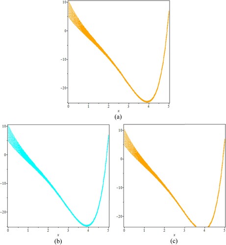
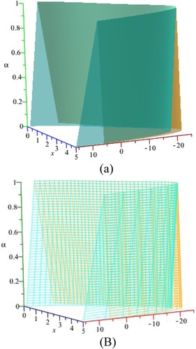
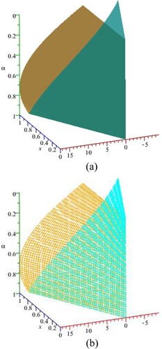
Here, we discuss the superiority of the numerical method SFQM1 over existing method SFQN1 in the literature in terms of efficiency, residual errors and computational time in seconds. The approximate solutions to the TFNSEs for various values of the fuzzy parameter r are shown in Tables 1(a) and 2(a), and the comparison of the exact and approximate solutions to the TFBVPs–I and TFBVP–II is shown in Tables 3(a) and 4(a). In terms of iterations, residual error computation time in seconds (CPU), and computational order of convergence, Tables 1(b)–4(b) demonstrate that our recently created approach, SFQM1, is more effective than SFQN1. The approximate numerical solution for the TFSLEs and TFSNEs utilized in examples 1 and 2 is shown in Figures 1(a–f)–2 using the SFQM1 and SFQN1 methods. The exact and approximate solutions to the TFBVPs-I and TFBVP-II are compared in Figure 3–6. It is evident from all of Figures 1–6 that SFQM1 exhibited better convergence behaviour than SFQN1 in terms of efficiency and errors.

Figure 1. (a–f) The numerical approximate solutions of the triangular Fuzzy nonlinear system of equations used in Example 1 via SFQM1, SFQN-methods. To obtain initial guess, we use above system for $r=0$ and $r=1,$ therefore, (a) approximate positive solution of $x_1$, (b) approximate positive solution of $x_2$ (c) approximate positive solution of $x_3$, (d) approximate positive solution of $x_4$, (e) approximate positive solution of $x_5$, and (f) combine solution of (TFSLEs)-1.

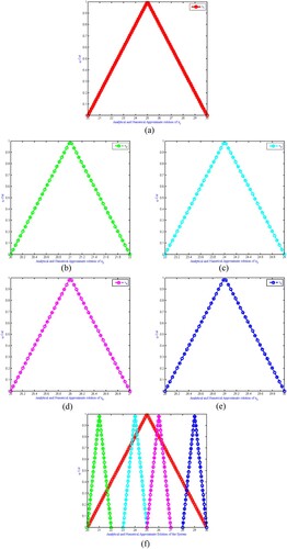
Figure 2. The numerical approximate positive solutions of the triangular Fuzzy nonlinear system of equations used in Example 2 via SFQM1, SFQN-methods.

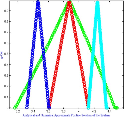
Figure 3. (a) The exact and approximate solutions for $y^L$, (c) The solution for $y^U$. The numerical approximate solution to the fuzzy boundary value problem is the same as the exact answer, as shown in (b, d). Exact solution of $y^L$, approximate solution of $y^L$, (c) exact solution of $y^U$, (d) approximate solution of $y^U$.

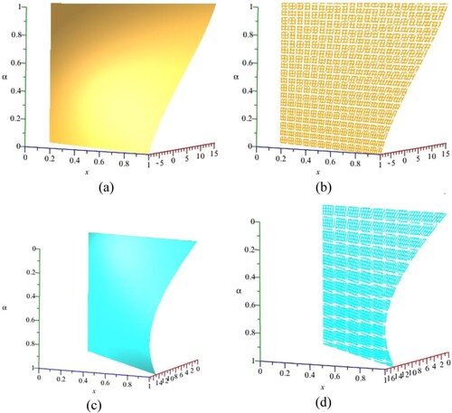
Figure 4. (a,b) The exact and numerical approximate solutions obtained using the SFQM1-iterative method. This figure clearly indicates that the approximate solution matched the actual solution. (a) Exact solution of TFBVP-1 and (b) approximate solution of TFBVP-1.

Figure 5. (b) The exact and approximate solutions for $y^L$, (c) The solution for $y^U$. The numerical approximate solution to the fuzzy boundary value problem is the same as the exact answer, as shown in (a). (a) Combine solution of $y^L\text{ and }{y}^U$, (b) approximate solution of $y^L$, (c) approximate solution of $y^U$.

Figure 6. (a, b) The exact and numerical approximate solutions obtained using the SFQM1-iterative method. This figure clearly indicates that the approximate solution matched the actual solution. (a) Exact solution of TFBVP-II and (b) approximate solution of TFBVP-II.

Conclusion

We developed a highly efficient numerical iterative scheme for solving triangular fuzzy linear and nonlinear systems of equations in this paper. Numerical test examples and two FBVP solutions illustrating the practical performance and dominance efficiency of the SFQM1 approach over the SFQN1 method on the same number of iterations. In comparison to the SFQN1 approach, the numerical results of SFQM1 methods are better in terms of absolute error and CPU time, as shown in Tables 1(a,b)–4(a,b) and Figures 1–6. Using the same methodologies as described in this article, and using technique of weight function we can construct optimal fourth-order efficient numerical iterative methods for solving systems of fuzzy linear and nonlinear equations using more generalized fuzzy numbers, i.e. intuitionistic fuzzy number [13], trapezoidal fuzzy number [37], bipolar fuzzy number [40], hesitant fuzzy number [42–44], etc.

Disclosure statement

No potential conflict of interest was reported by the author(s).

References

- Zadeh LA. Fuzzy sets. Inf Control. 1965;8:338–353.
- Zadeh LA. The concept of a linguistic variable and its application to approximation reasoning. Inf Sci. 1975;3:199–249.
- Dubois D, Prade H. Operations on fuzzy numbers. J Syst Sci. 1978;9:613–626.
- Dubois D, Prade H. Fuzzy sets and systems: theory and application. New York: Academic Press; 1980.
- Mizumoto M, Tanaka K. The four operations of arithmetic on fuzzy numbers. Syst Comput Controls. 1976;7(5):73–81.
- Mizumoto M, Tanaka K. Some properties of fuzzy numbers. In: Gupta MM, Ragade RK, Yager RR, editors. Advances in fuzzy Set theory and applications. Amsterdam: North-Holland; 1979. p. 156–164.
- Chang SSL, Zadeh LA. On fuzzy mapping and control. IEEE Trans Syst Man Cybern. 1972;2:30–34.
- Nahmias S. Fuzzy variables. Fuzzy Sets Syst. 1978;12:97–111.
- Goetschel R, Voxman W. Elementary calculus. Fuzzy Sets Syst. 1986;18:31–43.
- Moghadam KG, Ghanbari R, Amiri NM. Duality in bipolar triangular fuzzy number quadratic programming problems. In Proceedings of the International Conference on Intelligent Sustainable Systems, Palladam, Tirupur, India, 7–8 December 2017; pp. 1236–1238.
- Congxin W, Ming M. On embedding problem of fuzzy number spaces. Fuzzy Sets Syst. 1991;44:33–38.
- Puri ML, Ralescu D. Differential for fuzzy function. J Math Anal Appl. 1983;91:552–558.
- Keyanpour M, Akbarian T. Solving intuitionistic Fuzzy nonlinear equations. J Fuzzy Set Value Anal. 2014;2014:1–6.
- Buckley JJ, Qu Y. Solving linear and quadratic fuzzy equation. Fuzzy Sets Syst. 1990;38:43–59.
- Buckley JJ, Qu Y. On using a-cuts to evaluate equations. Fuzzy Sets Syst. 1990;38:309–312.
- Buckley JJ, Qu Y. Solving fuzzy equations: a new solution concept. Fuzzy Sets Syst. 1991;39:291–301.
- Buckley JJ, Qu Y. Solving systems of linear fuzzy equations. Fuzzy Sets Syst. 1991;43:33–43.
- Jajarmi A, Baleanu D, Zarghami KV, et al. A general fractional formulation and tracking control for immunogenic tumor dynamics. Math Methods Appl Sci. 2022;45(2):667–680.
- Erturk VS, Godwe E, Baleanu D, et al. Novel fractional-order Lagrangian to describe motion of beam on nanowire. Acta Phys Pol A. 2021;140(3):265–272.
- Jajarmi A, Baleanu D, Zarghami Vahid K, et al. A new and general fractional Lagrangian approach: a capacitor microphone case study. Results Phys. 2021;31:104950.
- Baleanu D, Abadi MH, Jajarmi A, et al. A new comparative study on the general fractional model of COVID-19 with isolation and quarantine effects. Alexandria Eng J. 2022;61(6):4779–4791.
- Kumar A, Malik M, Sajid M, et al. Existence of local and global solutions to fractional order fuzzy delay differential equation with non-instantaneous impulses. AIMS Math. 2022;7:2348–2369.
- Khan MB, Srivastava HM, Mohammed PO, et al. Fuzzy-interval inequalities for generalized convex fuzzy-interval-valued functions via fuzzy Riemann integrals. AIMS Math. 2022;7:1507–1535.
- Abbasbandy S, Ezzati R. Newton's method for solving system of fuzzy non-linear equations. Appl Math Comput. 2006;175(2):1189–1199.
- Allahviranloo T, Asari S. Numerical solution of fuzzy polynomial by Newton-Raphson method. J Appl Math Islam Azad Univ Lahijan. 2011;7(4 (27)):17–44.
- Mosleh M. Solution of dual fuzzy polynomial equations by modified Adomian decomposition method. Fuzzy Inf Eng. 2013;5:45–56.
- Koam A, Akram M, Muhammad G, et al. LU decomposition scheme for solving m-Polar Fuzzy system of linear equations. Math Probl Eng. 2020;2020:1–19.
- Akram M, Muhammad G, Koam ANA, et al. Iterative methods for solving a system of linear equation in bipolar fuzzy environment. Mathematics. 2019;7(728):1–25.
- Sulaiman IM, Mamat M, Waziri MY, et al. Solving fuzzy nonlinear equation via levenberg-marquardt method. Far East J Math Sci. 2018;103:1547–1558.
- Ma J, Feng G. An approach to H1 control of fuzzy dynamic systems. Fuzzy Sets Syst. 2003;137:367–386.
- Cho YJ, Huang NJ, Kang SM. Nonlinear equations for fuzzy mapping in probabilistic normed spaces. Fuzzy Sets Syst. 2000;110:115–122.
- Dennis JE, Schnabel RB. Numerical methods for unconstrained optimization and nonlinear equations. Hoboken, NJ: Prentice-Hall; 1983.
- Fang J. On nonlinear equations for fuzzy mappings in probabilistic normed spaces. Fuzzy Sets Syst. 2002;131:357–364.
- Shiri B, Irina P, Alijani Z. Classical approximation for fuzzy Fredholm integral equation. Fuzzy Sets Syst. 2021;404:159–177.
- Zimmermann HJ. Fuzzy sets theory and its application. Dordrecht: Kluwer Academic Press; 1991.
- Yao JS, Lin FT. Constructing a fuzzy flow-shop sequencing model based on statistical data. Int J Approximation Reason. 2002;29:215–234.
- Rafiq N, Yaqoob N, Kausar N, et al. Computer-Based Fuzzy numerical method for solving engineering and Real-World Applications. Math Probl Eng. 2021;2021:1–13.
- Mikaeilvand N, Noeiaghdam Z, Noeiaghdam S, et al. A novel technique to solve the fuzzy system of equations. Mathematics. 2020;8(5):850.
- Saqib M, Akram M, Shahida B. Certain efficient iterative methods for bipolar fuzzy system of linear equations. J Intell Fuzzy Syst. 2020;39(3):1–15.
- Akram M, Muhammad G, Allahviranloo T. Bipolar fuzzy linear system of equations. Comput Appl Math. 2019;38(69):1–29.
- Akram S, Shams M, Rafiq N, et al. On the stability of Weierstrass type method with King's correction for finding all roots of non-linear function with engineering application. Appl Math Sci. 2020;14(10):461–473.
- Qian G, Wang H, Feng X. Generalized hesitant fuzzy sets and their application in decision support system. Knowl Based Syst. 2013;37:357–365.
- Rasham T, Shabbir MS, Agarwal P, et al. On a pair of fuzzy dominated mappings on closed ball in the multiplicative metric space with applications. Fuzzy Sets Syst. 2022;437:81–96.
- Bataineh M, Alaroud M, Omari SA, et al. Series representations for uncertain fractional IVPs in the Fuzzy conformable fractional sense. Entropy . 2021;23(12):1646.