
 ?Mathematical formulae have been encoded as MathML and are displayed in this HTML version using MathJax in order to improve their display. Uncheck the box to turn MathJax off. This feature requires Javascript. Click on a formula to zoom.
Abstract
Finite-sum problems appear as the sample average approximation of a stochastic optimization problem and often arise in machine learning applications with large scale data sets. A very popular approach to face finite-sum problems is the stochastic gradient method. It is well known that a proper strategy to select the hyperparameters of this method (i.e. the set of a-priori selected parameters) and, in particular, the learning rate, is needed to guarantee convergence properties and good practical performance. In this paper, we analyse standard and line search based updating rules to fix the learning rate sequence, also in relation to the size of the mini batch chosen to compute the current stochastic gradient. An extensive numerical experimentation is carried out in order to evaluate the effectiveness of the discussed strategies for convex and non-convex finite-sum test problems, highlighting that the line search based methods avoid expensive initial setting of the hyperparameters. The line search based approaches have also been applied to train a Convolutional Neural Network, providing very promising results.
1. Introduction
In this paper, we consider the following optimization problem
(1)
(1)
where each
is differentiable with L-Lipschitz continuous gradient. We are especially interested in the case where the number of components N is very large, and, hence, the adoption of stochastic gradient methods is convenient since they exploit either a single gradient
or a very limited number of them at each iteration, rather than the entire gradient
. The study of the minimization problem (Equation1
(1)
(1) ) is relevant since it often arises in machine learning applications where it is known as empirical risk minimization. In this framework, N represents the number of samples and
is the single cost function corresponding to the ith sample.
A classical stochastic approach to solve (Equation1(1)
(1) ) is the mini batch stochastic gradient (SG) method [Citation1,Citation2], which, given
, is defined as
(2)
(2)
with
. Here
is a randomly chosen subset of
whose cardinality is denoted by
and
is a positive learning rate. The mini batch size
can be either a priori fixed or allowed to vary during the iterations.
It is well known in the literature that both the convergence properties and the practical performance of the algorithm (Equation2(2)
(2) ) are strongly influenced by the learning rate selection rule. In this paper, we discuss some techniques to choose the sequence of the learning rate
in combination with proper strategies to fix the mini batch size along the iterative process. We compare standard learning rate selection rules to line search based approaches which exploit a convenient increase of the mini batch size aimed at imposing some useful properties on the stochastic directions. An extensive numerical experimentation enables to evaluate the effectiveness of the considered strategies for convex and non-convex test problems. The behaviour of the discussed approaches is also evaluated on the problem arising in training a Convolutional Neural Network (CNN) for multi-classification, highlighting the stability properties of the line search strategies with respect to the hyperparameter setting.
2. Learning rate selection rules for stochastic gradient method
In this section, we discuss several possibilities to choose the learning rate in the SG scheme (Equation2(2)
(2) ) for both the fixed and the variable mini batch size cases.
2.1. Fixed mini batch size
For a deep survey on the convergence results of the SG scheme (Equation2(2)
(2) ) with fixed mini batch size
, the reader is referred to [Citation2]. However, it is worth to recall that, under the assumption that the gradient of the objective function is Lipschitz continuous with parameter L and some additional conditions on the first and second moments of the stochastic gradient, when the positive learning rate satisfies
, for a constant
depending on L, the expected optimality gap for strongly convex objective functions, or the expected sum of gradients for general objective functions, asymptotically converges to values proportional to
. Roughly speaking, if the learning rate is sufficiently small, the method generates iterates in the neighbourhood of the optimum or the stationary point. Nevertheless, the constants related to the above mentioned assumptions, such as the Lipschitz parameter L, are either unknown or not easy to approximate. For this reason, these results do not give an idea of how to select the learning rate. Moreover a too small value of this hyperparameter can give rise to a very slow learning process. As a consequence, the learning rate is often manually tuned in the practice by means of an expensive trial and error procedure. Furthermore, we recall that, under the selection of a suitable diminishing learning rate
and a fixed mini batch size, the expected value of the optimality gap generated by the SG method (Equation2
(2)
(2) ) for strongly convex objective functions, or the expected sum of gradients for general objective functions, converges to 0 at a sublinear rate
[Citation2]. Unfortunately, to select a diminishing sequence
is not efficient as well and the starting value of the learning rate
has to satisfy suitable assumptions.
An attempt to overcome this difficulty has been made in [Citation3,Citation4] where the Barzilai-Borwein (BB) rule, very often exploited to select the learning rate for the deterministic gradient methods, has been adapted to the stochastic setting. However, unlike in the deterministic framework, the generalized BB update requires either proper smoothing technique [Citation4] to diminish the current learning rate while running the algorithm or a thresholding procedure on it, based on user dependent bounds
[Citation3] to avoid instability and ensure the convergence.
2.2. Variable mini batch size
For twice differentiable objective function such that ,
, a way to obtain the linear convergence for the SG method (Equation2
(2)
(2) ) consists in increasing the size of the current mini batch
at a geometric rate [Citation5], provided that the learning rate is fixed as a positive value bounded from above by
. This approach has two drawbacks: the size of the mini batch increases too rapidly and the constant L is typically not known, as already said before. In order to overcome these drawbacks we report in the following two strategies developed very recently [Citation6,Citation7].
In [Citation6] the authors suggest to increase the mini batch size in (Equation2(2)
(2) ) on the basis of two conditions imposed on the stochastic directions. These conditions, called inner product test and orthogonality test, guarantee that the search directions computed on a mini batch of suitable size are descent directions with high probability:
(3)
(3)
(4)
(4)
where θ and
are prefixed positive values. For twice differentiable objective functions such that
, if the inner product test and the orthogonality test are fulfilled and the learning rate is fixed at each iteration and bounded from above by a constant depending on L, θ and
, then the SG scheme (Equation2
(2)
(2) ) is linearly convergent. Under the same assumptions on the mini batch size and the learning rate, weaker theoretical convergence properties hold for more general objective functions. Since these results strongly depend on the knowledge of the Lipschitz parameter L, a line search procedure has been devised for its numerical estimation. The resulting algorithm is called the Adaptive Sampling Method (ASM).
In the deterministic setting [Citation8–11], the BB rule has been proved to give a local estimate of the inverse of the Lipschitz constant of . Motivated by this observation, we decide to also consider a modified version of ASM, called ASM-BB1, where the learning rate is no more fixed by means of the line search procedure but through the BB rule developed for the stochastic setting in [Citation4]. The value for
is kept fixed until the size of the mini batch changes in according to the conditions (Equation3
(3)
(3) ) and (Equation4
(4)
(4) ). When the size of the mini batch is increased by the inner product test and the orthogonality test, a new BB learning rate is computed. This version of ASM is denoted by ASM-BB1 in the following. In [Citation12] a similar approach to that of ASM-BB1 is adopted. The authors developed two SG methods of the form (Equation2
(2)
(2) ) where the increase of the mini batch size is controlled by means of (Equation3
(3)
(3) ) and (Equation4
(4)
(4) ) and the learning rate is computed through two different generalized BB rules based on the so called Ritz-like and harmonic Ritz-like values, respectively. Hereafter, these approaches will be denoted by ASM-A-R and ASM-AA-R, respectively.
An idea similar to that on which ASM is based, has been followed in [Citation7]. Here the authors developed a proximal stochastic gradient algorithm to face a regularized version of problem (Equation1(1)
(1) ); however, if the function to minimize is defined as in (Equation1
(1)
(1) ), such algorithm belongs to the class of mini batch SG methods (Equation2
(2)
(2) ) with variable mini batch size. In more detail, the mini batch
is selected such that the variance of the stochastic gradients is dynamically reduced along the iterative process, namely,
(5)
(5)
where
denotes the conditional expected value with respect to the σ-algebra generated by the information collected before iteration k, i.e. assuming
given. Hereafter we provide two convergence results for the scheme (Equation2
(2)
(2) ) combined with condition (Equation5
(5)
(5) ): the first one is more general since it allows the objective function to be non-convex. This convergence analysis is different to the one developed in [Citation7] and it is especially tailored for the SG method (Equation2
(2)
(2) ) applied to the class of optimization problems (Equation1
(1)
(1) ). Before presenting the main results, we need to recall a classical result from stochastic analysis.
Lemma 2.1
[Citation13, Lemma 11]
Let ,
,
,
be nonnegative random variables and let
where
denotes the conditional expectation for the given
,
,
,
. Then
where
is some random variable.
Theorem 2.2
Let be the sequence generated by (Equation2
(2)
(2) ) with
If
is an unbiased estimate of
and condition (Equation5
(5)
(5) ) holds, then
Proof.
In view of (Equation2(2)
(2) ) and the L-Lipschitz continuity of
, we have that
(6)
(6)
By taking the conditional expectation on both sides of inequality (Equation6
(6)
(6) ) and recalling that
and, hence,
, we obtain that
Since
and condition (Equation5
(5)
(5) ) holds, Lemma 2.1 can be invoked. Therefore
and the theorem is proved.
The above theorem enables us to affirm that if has a limit point, then this point is a stationary point for F a.s.
Theorem 2.3
Let be the sequence generated by (Equation2
(2)
(2) ) with
If
is an unbiased estimate of
, condition (Equation5
(5)
(5) ) holds true, the function F is convex and the solution set
of problem (Equation1
(1)
(1) ) is not empty, then
converges to a solution of (Equation1
(1)
(1) ) a.s.
Proof.
Let . We observe that
(7)
(7)
where the third equality follows from the definition of
in (Equation2
(2)
(2) ). By taking the conditional expectation on both sides of inequality (Equation7
(7)
(7) ), we can write that
where the first inequality follows from the convexity of F and the second inequality follows from the fact that the L-Lipschitz continuity of
implies that
. From the hypotheses on
and the conditional expected value of the variance of the stochastic gradient, Lemma 2.1 can be applied and we can state that the sequence
converges a.s.
Next we prove the almost sure convergence of the sequence by following a strategy similar to the one employed in [Citation14, Theorem 2.1]. Let
be a countable subset of the relative interior
that is dense in
. From the almost sure convergence of
,
, we have that for each i, the probability
. Therefore, we observe that
where the inequality follows from the union bound, i.e. for each i,
is a convergent sequence a.s. For a contradiction, suppose that there are convergent subsequences
and
of
which converge to their limiting points
and
respectively, with
. By Theorem 2.2,
and
are stationary; in particular, since F is convex, they are minimum points, i.e.
. Since
is dense in
, we may assume that for all
, we have
and
are such that
and
. Therefore, for all
sufficiently large,
On the other hand, for sufficiently large j, we have
This contradicts with the fact that
is convergent. Therefore, we must have
, hence there exists
such that
.
The previous theorems show that the convergence of the sequence generated by algorithm (Equation2(2)
(2) ) can be obtained provided that condition (Equation5
(5)
(5) ) holds and the learning rate
is bounded by a constant depending on the Lipschitz constant of the gradient of the objective function. Since both these requirements seem difficult to be preserved in practice, we now detail how to select the stochastic gradients and the learning rate along the iterations in order to realize them. The resulting method is a Line search based Stochastic first order Algorithm (LISA) and it is stated in Algorithm 1. Some explanations are needed.
The variance of the search directions is controlled through a dynamic increase of the size of the mini batch as described in Step 1. In more detail, under the assumption that , there exists a constant value
such that
. Hence, for an arbitrary
, we have that [Citation15, p. 183]
This bound, when combined with a suitable rate of increase in
, enables to guarantee condition (Equation5
(5)
(5) ). Indeed, it is sufficient that
with
. Following a standard strategy [Citation2,Citation5,Citation6], the first term of the above condition can be approximated by the sample variance which, at the kth iteration, is defined as
Hence, as a practical counterpart of condition (Equation5
(5)
(5) ), at each iteration we force that
(9)
(9)
where
is any nonnegative sequence such that
. In view of inequality (Equation9
(9)
(9) ), the variance can be monitored by a proper increase of the sample size
: whenever condition (Equation9
(9)
(9) ) is not satisfied, the sample size
is increased. As for the selection of the learning rate, since the Lipschitz constant of
is often not known, a line search procedure on the sampled objective function is adopted in order to estimate it. Indeed, given
and by assuming that all the
have Lipschitz-continuous gradients with Lipschitz constant L, the gradient estimate
is Lipschitz continuous with the same Lipschitz parameter and it holds that
(10)
(10)
In view of (Equation10
(10)
(10) ) and denoted by
, we require that
satisfies the following inequality
which can be rewritten as in (8). If the value of
does not guarantee the validity of (8), then it is reduced by a factor
. The line search strategy (8) is well defined: indeed as soon as
, condition (8) is automatically satisfied. Finally, we point out that the ASM method and the LISA one shares the same line search requirement on the learning rate.
3. Numerical experiments
In this section, we present two different kinds of numerical experiments. In the first one, we consider a binary classification problem, using both convex and non-convex loss functions with several literature datasets. In the second one, we train an artificial neural network tailored for a multiple classification problem.
3.1. Binary classification
This section is devoted to a comparison of the previously discussed strategies for solving binary classification problems. In particular, we consider the following algorithms:
the standard SG method with a fixed size for the mini batch and the learning rate initialized by an optimal hand-tuned value and then properly decreased during the iterations;
the SG method with a fixed size for the mini batch and the learning rate selected by means of the BB updating rule as defined in [Citation3]; hereafter this approach has been denoted by BB1;
the ASM method developed in [Citation6];
the ASM-BB1 method discussed above;
the LISA method described in Algorithm 1.
To evaluate the effectiveness of the methods under analysis in solving problem (Equation1(1)
(1) ), we build a binary classifier in the case of four data sets. Table shows the details of these data sets and the cardinality of the train and the test sets. The datasets W8A, IJCNN1 are downloadable from https://www.csie.ntu.edu.tw/cjlin/libsvmtools/, whereas MNIST is available at https://yann.lecun.com/exdb/mnist/ and CHINA0 at https://www.causality.inf.ethz.ch/home.php.
Table 1. Features of each data set.
To consider different instances of the problem (Equation1(1)
(1) ), two convex loss functions and two non-convex loss functions are used as objective function
; in particular, by denoting with
the feature vector and with
the class label of the ith sample,
assumes one of the following forms:
logistic regression (LR) loss:
smooth hinge (SH) loss:
nonconvex loss in 2-layer neural networks (NN):
logistic difference (LD) loss:
3.1.1. Hyperparameters setting
In the SG method, the mini batch has a fixed size equal to ; the learning rate is selected with the rule
, where
is the initial learning rate and j is the counter of the epochs. In particular, the initial learning rate is defined by
, where
is the optimal tuned value computed through a trial and error process by using
. The values of
for the considered test problems are shown in Table .
Table 2. Best tuned values of for the considered test problems.
In BB1 method, the mini batch size is fixed as and the first learning rate is set as
. Furthermore, the values of
and
are listed in Table . Similarly, the initial mini batch size and the initial learning rate of ASM-BB1 method are
and
, whereas Table shows the values of
and
for ASM-BB1.
Table 3. Values of and
for the BB1 method; in the thresholding procedure, these values are divided by the counter of the current epoch.
Table 4. Values of and
for the ASM-BB1 method.
In the ASM method, the initial mini batch size is set as whereas the initial learning rate is
; using the same notation of [Citation6], the setting of the other hyperparameters is
,
, r = 10,
,
and
. For the loss SH, θ is fixed as 0.9 for the data sets IJCNN and CHINA0.
In the LISA method, we set ,
,
and the attempt value of
to start the line search procedure (8) has been chosen as
, for the following iterations. In addition, the rule
guarantees the consistency with respect to the theoretical formulation.
It is worth to emphasize that both the ASM and the LISA algorithms are free from the expensive tuning of either an optimal value for the learning rate or proper bounds on it, unlike the SG, the BB1 and the ASM-BB1 approaches.
3.1.2. Results
The numerical experiments are carried out in Matlab on a 1.8 GHz Intel Core i7 processor. All the runs are carried out by varying random number generator and performing 10 trials keeping fixed the aforementioned hyperparameters. In order to estimate the optimality gap, namely
, for any test problem an approximate value
of the minimum is computed by a huge number of iterations of one of the considered methods.
For any numerical test, the following results are reported:
average and STandard Deviation (STD) of the optimality gap
evaluated on the train set, where
average and STD of the accuracy
In Tables and the results obtained for all the test problems are shown. We can conclude that the LISA method is competitive with respect to the other methods in terms of both optimality gap and accuracy.
Table 5. Results for the LR and SH loss functions.
Table 6. Results for the NN and LD loss functions.
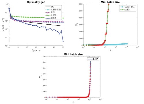
For a subset of the considered test problems, in Figures – we report the behaviour of the optimality gap with respect to the epochs for all the considered methods (top left panels); in the top right and bottom panels, the increase of the mini batch size is shown for ASM, ASM-BB1 methods and for LISA respectively. The mini batch size for ASM, ASM-BB1, and LISA is always significantly lower than the size of the considered data set. The red circles represent the learning rate reductions performed by the line search in ASM and LISA methods.
Figure 1. CHINA0 data set with LR loss: optimality gap (top left panel), increase of mini batch size in ASM and ASM-BB1 (top right panel) and increase of mini batch size in LISA (bottom panel).
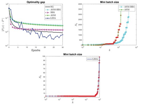
Figure 2. w8a data set with SH loss: optimality gap (top left panel), increase of mini batch size in ASM and ASM-BB1 (top right panel) and increase of mini batch size in LISA (bottom panel).
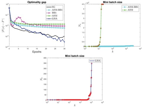
Figure 3. IJCNN data set with NN loss: optimality gap (top lef panel), increase of mini batch size in ASM and ASM-BB1 (top right panel) and increase of mini batch size in LISA (bottom panel).
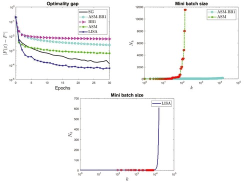
Figure 4. MNIST data set with LD loss: optimality gap (top left panel), increase of mini batch size in ASM and ASM-BB1 (top right panel) and increase of mini batch size in LISA (bottom panel).
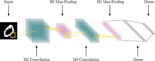
3.2. A case study: image classification via a convolutional neural network
A meaningful case study is the training of a multiclassifier on a CNN. The network is composed of an input layer, two sequences of convolutional and max-pooling layers, a fully connected layer, and an output layer (see Figure ). In particular, the first convolutional layer is composed by 64 filters (each of them of size ), the second convolutional layer is composed by 32 filters (each of them of size
) and both the max-pooling layers are
. At the end of each inner convolutional layer, there is a sigmoid activation function, whereas the output layer has a softmax function and the loss is given by the cross entropy function. By this CNN, we build a 10-class classifier for the MNIST data set. To avoid the overfitting phenomenon, a ridge regularization is added to the loss, with a regularization parameter equal to
. In addition to the simple SG scheme, we also present a comparison with the ASM-A-R and ASM-AA-R methods recalled in Section 2.2 and developed in [Citation12]. For the SG method, the size of the mini batch, is set as
; in ASM-A-R and ASM-AA-R methods, the size of the initial mini batch is
.
Figure 5. Artificial neural network structure.
The numerical experiments described in the following were carried out in Matlab on Intel(R) Core(TM) i7-6700 CPU @ 3.40GHz with 8 CPUs.
Since we are working with a CNN, the choices of both the learning rate and the mini batch size are particularly important and critical. On the one hand, the choice of the mini batch size is subject to memory constraints. Particularly, taking into account the memory resources on the architecture, the maximum possible number of examples for a single sample of the considered dataset is near 8000. On the other hand, to select a good learning rate is crucial to obtain a fast learning phase and to avoid divergence phenomena.
On the left panel of Figure , we show the accuracy obtained by the SG method on the test set in the first 5 epochs with different values of the learning rate. It is evident that the choice of the learning rate is critical. In more detail, a too small learning rate (dashed black line) leads to a very slow learning phase, while a too large learning rate (dashed magenta line with solid dot) makes the algorithm divergent; indeed an accuracy of 0.1 in a 10-class case is total randomness. Especially in neural networks context, this initial process of finding a good learning rate involves a high number of attempts, which are computationally expensive. On the other hand, the adaptive methods present a good performances in both cases, as highligthed on the right panel of Figure . This behaviour also occurs in the case of the LISA method. Indeed, in the following we can show that very stable and accurate results can be obtained even with different settings of the hyperparameters. The initial mini batch size and the initial learning rate
are always set equal to 10 and 1, respectively. Moreover, we remark that when the condition (8) is not satisfied, the value of
is reduced by a factor
; on the contrary, the starting value of the learning rate for the successive line search is incremented by a factor τ, with
. The condition
avoids an unnecessary number of line searches. For the mini batch size increasing, the rule
guarantees the consistency with respect to the theoretical formulation and, by means of the C value, the increase rate of the sample is driven. Numerical experiments were conducted with different combinations of the above hyperparameters. Table reports their values for the considered configurations.
Figure 6. CNN accuracy in the SG case.
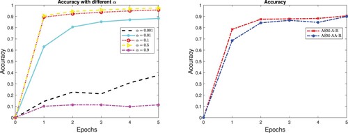
Table 7. Possible different configurations for the LISA method.
As shown in Figure , the LISA scheme is very robust toward the choice of the hyperparameters. Indeed, for all the configurations explored, it achieves an accuracy comparable to that obtained by SG equipped with the optimal learning rate and constant mini batch size. For completeness we report in Table the accuracy achieved for each of the five epochs by the LISA method (measured on the test set) and the corresponding loss values on the train set in Table .
Figure 7. Accuracies for LISA method in the CNN case, with different hyperparameter configuration.
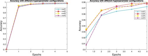
Table 8. Accuracies obtained by LISA method in the CNN case, with different hyperparameter configurations.
Table 9. Loss values for LISA method in the CNN case, with different hyperparameter configurations.
A further remark is related to the sample size reached at the end of five epochs. As shown in Table , the final sample size is only slightly over a hundred, thus remaining far from the hardware memory constraint. Furthermore, for comparison with ASM-A-R and ASM-AA-R methods, we notice that the sample size increases up to a maximum of 204 and 182 respectively.
Table 10. Final mini batch cardinality for LISA method in the CNN case, with different hyperparameter configurations.
4. Conclusions
In this paper, we discussed several updating rules to choose the learning rate in stochastic gradient methods to face finite-sum problems. We considered standard and line search based learning rate selection techniques and we compared them in combination with proper strategies to fix the mini batch size along the iterative process. The stochastic gradient algorithms which exploit a line search procedure to determine the learning rate have performance comparable to that of the standard stochastic gradient methods but they avoid the computational expensive trial and error phase to manually adjust the learning rate (and other hyperparameters) needed instead by the latter ones. Moreover the line search based schemes do not even require the setting of proper bounds on the learning rate. For these reasons, the line search approaches appear preferable and they are worthy of further investigation.
Disclosure statement
No potential conflict of interest was reported by the author(s).
Additional information
Funding
References
- Robbins H, Monro S. A stochastic approximation method. Ann Math Stat. 1951;22(3):400–407.
- Bottou L, Curtis FE, Nocedal J. Optimization methods for large-scale machine learning. SIAM REV. 2018;60(2):223–311.
- Liang J, Xu Y, Bao C, et al. Barzilai–Borwein-based adaptive learning rate for deep learning. Pattern Recognit Lett. 2019;128:197–203.
- Tan C, Ma S, Dai YH, et al. Barzilai–Borwein step size for stochastic gradient method. In: Lee D, Sugiyama M, Luxburg U, Guyon I, Garnett R, editors. Advances in neural information processing systems (NIPS2016), Barcelona, Spain; 2016. p. 29.
- Byrd RH, Chin GM, Nocedal J, et al. Sample size selection in optimization methods for machine learning. Math Program. 2012;134(1):127–155.
- Bollapragada R, Byrd R, Nocedal J. Adaptive sampling strategies for stochastic optimization. SIAM J Optim. 2018;28(4):3312–3343.
- Franchini G, Porta F, Ruggiero V, et al. A line search based proximal stochastic gradient algorithm with dynamical variance reduction. Optimization online; 2022.
- Barzilai J, Borwein JM. Two-point step size gradient methods. IMA J Numer Anal. 1988;8:141–148.
- Dai YH, Liao LZ. R-linear convergence of the Barzilai and Borwein gradient method. IMA J Numer Anal. 2002;22(1):1–10.
- Dai YH, Fletcher R. On the asymptotic behaviour of some new gradient methods. Math Program. 2005;103:541–559.
- di Serafino D, Ruggiero V, Toraldo G, et al. On the asymptotic behaviour of some new gradient methods. Appl Math Comput. 2018;318:176–195.
- Franchini G, Ruggiero V, Zanni L. Ritz-like values in steplength selections for stochastic gradient methods. Soft Comput. 2020;24:17573–17588.
- Polyak BT. Introduction to optimization. New York: Optimization Software; 1987.
- Poon C, Liang J, Schoenlieb C. Local convergence properties of SAGA/Prox-SVRG and acceleration. In: Dy J and Krause A, editors. Proceedings of the 35th International Conference on Machine Learning. PMLR; 2018. Vol. 80. p. 4124–4132.
- Freund JE. Mathematical statistics. Englewood Cliffs, NJ, USA: Prentice-Hall; 1962.