Disturbance observer-based fuzzy adaptive optimal finite-time control for nonlinear systems

Abstract

This paper investigates the issue of disturbance observer-based fuzzy adaptive optimal finite-time control in light of the backstepping approach for strict-feedback nonlinear systems with bias fault term and full state constraints. Considering that external disturbance and bias fault signal can affect the stability of control and control quality, a disturbance observer is constructed to track the external disturbances and bias fault online. A disturbance observer-based finite-time control strategy is proposed to achieve optimized control by utilizing the fuzzy logic system approximation-based adaptive dynamic programming method under the critic-actor framework. The purpose of the critic is to evaluate control performance and the role of the actor is to execute control behaviour. In addition, it is proved that the proposed fuzzy adaptive optimal finite-time scheme not only realizes all signals in closed-loop system are bounded, but also ensures that system states are restricted within specific sets. Finally, simulation results are shown to demonstrate the effectiveness of the proposed control strategy.

Keywords:

• Adaptive dynamic programming
• fuzzy adaptive optimal finite-time control
• external disturbance observer
• state observer

Mathematics Subject Classifications:

• 34H05
• 93C10
• 93C42

1. Introduction

In the past few decades, the research on controller designing for nonlinear systems speedy developed neural networks and fuzzy approximation characteristics [1–4]. The incipient control strategies facilitate the control objectives for nonlinear systems are realized in a infinite time, which means that the stability of systems fails to be guaranteed in a finite time. However, in practical problems, it is imperative to achieve superior control performance in a finite time.

Dissimilar to asymptotic stability, finite-time stability converges fast without the requirement of long-term transient response, so it is widely concerned and applied to practical systems such as aircraft flight systems [5], cart-pole systems [6], teleoperation systems [7] and so on. Bhat and Bernstein [8] explained finite-time stability based on Lyapunov theory and constructed feedback controller for nonlinear systems to achieve finite-time stability. Qiu et al. [9] established a fuzzy finite-time controller for nonlinear systems and realized the tracking error is limited to a bounded set. Li et al. [10] studied the problem of finite-time containment control involving unmeasurable states for nonlinear multiagent systems with input delay. Zhang et al. [11] designed an adaptive fuzzy control strategy based on finite-time stability criterion for nonlinear systems with unavailable states, in which all states are confined to restricted sets. Meng et al. [12] developed a finite-time quantized controller for dealing with the nonlinear systems contingent on unknown control directions, which constructed state and disturbance observers simultaneously. Sui et al. [13] constructed an event-trigger adaptive finite control scheme by combining backstepping and varying threshold condition for stochastic nonlinear systems with unmodelled dynamics. Saravanakumar et al. [14] first investigated the finite-time stability problem. The authors in [15–17] studied the issue of finite-time control for nonlinear systems in accordance with full-state constraints. Nguyen et al. [18] introduced a fuzzy control strategy for parallel manipulators to guarantee that the error of tracking converges fast in a finite time. Wang et al. [19] constructed a finite-time control algorithm for stochastic nonlinear systems with actuator faults. Nevertheless, the above literature take the finite time into account and the designed control strategies ensure that the control objective can be achieved within the finite time. However, these literature do not involve the optimal control to deal with the problem of resource consumption.

In recent years, optimal control has been a striking topic, and it is concerned with establishing control strategies to achieve control objectives with the least resources in regard to optimal policy. In other words, the goal of optimal control is to consume the least amount of resources to achieve the control objective. For nonlinear systems, it is noteworthy that the resolve of Hamilton–Jacobi–Bellman (HJB) equation is imperative in the control process, but it is problematic to get analytic solutions because of the dynamic uncertainty and strong nonlinearity in the actual control. To overcome this problem, the dynamic programming (DP) was developed by Bellman [20]. Noted that although DP is an effective tool for obtaining optimal solutions, it is prone to the curse of dimensionality, that is, increasing dimensions bring computational disasters. Adaptive dynamic programming (ADP)-based algorithms were demonstrated to efficiently conquer the problem. Werbos [21] developed ADP for discrete systems and Abu-Khalaf and Lewis [22] proposed ADP control scheme for continue-time nonlinear systems where the neural networks approximation structure was established to estimate the value function of the HJB equation. Vamvoudakis et al. [23] developed an online actor-critic scheme combined with neural networks for continue-time systems. Wen et al. [24] designed an optimized formation control strategy in reference with identifier-actor-critic structure and approximation characteristic of fuzzy logic systems. Li and Li [25] introduced a fuzzy adaptive optimal fault-tolerant control scheme for stochastic multiagent systems to incorporate Butterworth low-pass filter, which leverages to compensate for negative influence caused by nonlinear fault on the system. Wen et al. [26] reviewed the fuzzy adaptive optimized control issue subject to unmeasured states with nonlinear systems, in which the state observer satisfies the Hurwitz condition that sidestep constant designing. Lan et al. [27] introduced an adaptive optimal formation control technology for multiagent systems with unmeasurable states. Li et al. [28] designed a neural network adaptive optimized control algorithm exposing to immeasurable states and constrained states with nonlinear systems. The authors in [29–31] discussed the problem of adaptive optimal control for nonlinear systems. Wen et al. [32] built an adaptive optimal control scheme by virtue of identifier–critic–actor architecture. To achieve high precision control requirements, it is necessary to consider the influence of external disturbance on the system, which makes sense to design an optimal finite-time control strategy for the controlled system with external disturbance. However, the proposed approaches in [20–32] ignored the external disturbance in the controller system.

It is a prominent prospect to eliminate the influence of external disturbances on the systems [33–38]. Ji et al. [39] designed an adaptive fault-tolerant optimized formation control for multiagent systems with disturbances, in which a disturbance observer was constructed to alleviate the negative effects of external disturbance. Liu et al. [40] developed an adaptive control scheme for Markovian jump systems that suffer from external disturbances and actuator faults, in which external disturbances contain matched and mismatched part. Xu et al. [41] designed a neural network disturbance observer for strict-feedback systems to achieve good control performance in spite of unknown dynamics and time-varying disturbance. Song and Lewis [42] introduced a robust optimal control scheme with a disturbance observer to estimate disturbances for nonlinear systems. Zerari and Chemachema [43] studied the continuously stirred tank reactor systems containing external disturbances and introduced the compensator to confront the influence of external interference in the designed control strategy. Ran et al. [44] proposed a disturbance rejection optimal control for nonlinear systems, in which the perturbances and other uncertainties are estimated by the designed disturbance observer. Chen and Ge [45] presented an adaptive neural control strategy for nonlinear systems with unmeasured states, hysteresis and disturbances. However, the foregoing advancements rarely studied the optimized finite-time control problem based on fuzzy systems for nonlinear systems with full-state constraints and external disturbances.

Motivated by the aforementioned researches, this paper considers the fuzzy adaptive optimal finite-time control issue for nonlinear systems with full-state constraints, external disturbance and bias fault. Combining backstepping and ADP tricks, a fuzzy adaptive optimal finite-time control strategy is designed. The unknown system functions are approximated by the fuzzy logic system and disturbance observers are designed to solve the influence of external disturbances and bias fault signal. Virtual and actual controllers are introduced by being incorporated with actor-critic architecture and backstepping framework. The main contributions are summarized as follows.

1. In comparison with  [25,27,28], the designed scheme via actor-critic framework and finite-time stability theory can ensure the controller systems not only has a faster convergence rate and limits the tracking error derives within a temperate area of the origin in a finite time.

2. An disturbance observer-based fuzzy finite-time strategy based on actor-critic structure is proposed. Discriminating the control schemes in [26,32,46], it not only considers the full-state constraint for strict-feedback nonlinear systems but also addresses the effects of bias fault and external disturbance on the system by designing the disturbance observer.

The remainder of this article is organized as follows. In Section 2, the system description and preliminary knowledge are presented. Section 3 proposes an observer-based fuzzy optimal control scheme. Subsequently, stability analysis is given in Section 4. A simulation example is shown in Section 5. Finally, the conclusion is presented in Section 6.

2. Preliminaries and problem statement

2.1. System description

The strict-feedback nonlinear system consisting of unknown dynamics is formulated by (1) $\{\begin{array}{l}{\dot{x}}_i=x_{i+1}+{\varphi }_i\left({\overline{x}}_i\right)+D_1\left(t\right),\\ {\dot{x}}_n=u^A+{\varphi }_n\left({\overline{x}}_n\right)+D_n\left(t\right),\\ y\left(t\right)=x_1,1\le i\le n,\end{array}$(1) where ${\overline{x}}_i=[x_1,x_2,\dots ,x_i{]}^T\in {\mathbb{R}}^i$ ($i=1,\dots ,n$) represent the states vector of the system, $y\in \mathbb{R}$ is the control output. ${\varphi }_i$(${\overline{x}}_i$) $\in {\mathbb{R}}^i$ are the unknown functions and $D_i\left(t\right)$ denote the external disturbances where $i=1,\dots ,n$. All system states are restricted to a compact set, that is, $x_i<|k_{ic}|$ where $|k_{ic}|$ are positive constants with $i=1,2,\dots ,n$.

In actual engineering applications, the actuator bias faults often occur during the operation of the actuator. Thus we consider the actuator bias fault signal as (2) $u^A=u+u_f,$(2) where u denotes the control input and $u_f$ represents the actuator bias fault signal. Suppose $u_f$ is bounded and there is a constant F that $u_f\le F$.

Assumption 2.1

[39]

The external disturbances $D_i\left(t\right)$ are unknown and bounded, i.e. there exist real numbers $D_i^{\ast }$ and ${\overline{D}}_i$ satisfying $|{\dot{D}}_i\left(t\right)|\le D_i^{\ast }$ and $D_i\left(t\right)\le {\overline{D}}_i$ where $i=1,2,\dots ,n$.

Assumption 2.2

[25]

The reference trajectory $y_r$ is known and bounded, and the derivatives of the $y_r$, ${\dot{y}}_r\cdots y_r^n$ are bounded.

2.2. Finite-time theory

The following lemmas are beneficial to facilitate the design of the controller.

Lemma 2.1

[15]

For any positive numbers $C_1>0,C_2>0$, $0<\delta <1$, 0<l<1, there exist a $C^2$ function $V\left(x\right)$ satisfying (3) $V\left(x\right)\le -C_1{V}^{\delta }-C_{2}V+M,$(3) then the system is finite-time stable, where the setting time $T_0\le \frac{1}{C_2(1-\delta )}\ln \frac{C_2{V}^{1-\delta }\left(x_0\right)+l{C}_1}{C_2(\frac{M}{(1-l)C_1}{)}^{\frac{1-\delta }{\delta }}+l{C}_1}$.

Lemma 2.2

[29]

For any $\tau \in \mathbb{R}$, there exist an integer constant ξ and a positive constant $0<q\le 1$, one has (4) ${\left(\sum _{i=1}^n|\tau |\right)}^q\le \sum _{i=1}^n|\tau {|}^q\le n^{1-q}{\left(\sum _{i=1}^n|\tau |\right)}^q.$(4)

Lemma 2.3

[29]

There exists real variables $p_1$ and $p_2$ satisfying the following inequality: (5) $|p_1{|}^{r_1}|p_2{|}^{r_2}\le \frac{r_1}{r_1+r_2}{r}_3|p_1^{r_1+r_2}+\frac{r_2}{r_1}{r}_3^{\frac{-r_1}{r_2}}|p_2{|}^{r_1+r_2}.$(5) where $r_1$, $r_2$ and $r_3$ are positive constants.

2.3. Fuzzy logic system

A host of real-world systems exit unknown dynamics which affect the control performance, and fuzzy logic system approximation approach facilitates to solve the negative effect problem of unknown dynamics. The knowledge base constitutes IF–THEN rules which are stated in the following forms: $\begin{array}{rl}{R}^k:& \mathrm{I}\mathrm{f}{x}_1\mathrm{i}\mathrm{s}{G}_1^k,x_2\mathrm{i}\mathrm{s}{G}_2^k,\dots ,x_n\mathrm{i}\mathrm{s}{G}_l^k,\\ & \mathrm{t}\mathrm{h}\mathrm{e}\mathrm{n}y\mathrm{i}\mathrm{s}{Q}^k,k=1,2,\dots ,N,\end{array}$where $x=(x_1,x_2,\dots ,x_l{)}^T\in {\mathbb{R}}^l$ and y are the input and output of fuzzy logic system. $G_l^k$ and $Q^k$ represent fuzzy sets, and N denotes the number of rules. Then the fuzzy logic system can be described by (6) $y\left(x\right)=\frac{\sum _{k=1}^N{\overline{y}}^k\prod _{i=1}^l{\mu }_{G_i}^k\left(x_i\right)}{\sum _{k=1}^N\prod _{i=1}^l{\mu }_{G_i}^k\left(x_i\right)},$(6) where ${\mu }_{G_i}^k$ and ${\mu }_Q^k$ are fuzzy membership functions, and ${\overline{y}}^k=\underset{y\in R}{max}{\mu }_{Q^k}\left(y\right)$.

The basis functions are defined as (7) $S_k\left(x\right)=\frac{\prod _{i=1}^l{\mu }_{G_i}^k\left(x_i\right)}{\sum _{k=1}^N\prod _{i=1}^l{\mu }_{G_i}^k\left(x_i\right)}.$(7) Denote $\mathrm{\aleph }=({\mathrm{\aleph }}_1,{\mathrm{\aleph }}_2,\dots ,{\mathrm{\aleph }}_N{)}^T$, and $S\left(x\right)=\left(S_1\right(x),S_2(x),\dots ,S_k(x){)}^T$, and (6(6) $y\left(x\right)=\frac{\sum _{k=1}^N{\overline{y}}^k\prod _{i=1}^l{\mu }_{G_i}^k\left(x_i\right)}{\sum _{k=1}^N\prod _{i=1}^l{\mu }_{G_i}^k\left(x_i\right)},$(6) ) can be stated as follows: (8) $y\left(x\right)={\mathrm{\aleph }}^{T}S\left(x\right).$(8)

Lemma 2.4

[24]

Let $f\left(x\right)$ be a continuous function defined on compact set ℘. There exists a positive constant φ that satisfies the following inequality: (9) $\underset{x\in \mathrm{\wp }}{sup}|\varphi \left(x\right)-{\mathrm{\aleph }}^{T}S\left(x\right)|\le \phi .$(9)

By means of (9(9) $\underset{x\in \mathrm{\wp }}{sup}|\varphi \left(x\right)-{\mathrm{\aleph }}^{T}S\left(x\right)|\le \phi .$(9) ), the following fuzzy logic systems are served to approximate the functions ${\varphi }_i$ ($i=1,2,\dots ,n$): (10) ${\varphi }_i\left({\overline{x}}_i|{\hat{\mathrm{\aleph }}}_i\right)={\hat{\mathrm{\aleph }}}_i^T{S}_i\left({\overline{x}}_i\right),$(10) where ${\hat{\overline{x}}}_i$ represents the approximation of ${\overline{x}}_i$ and ${\hat{\mathrm{\aleph }}}_i$ denotes the estimations of ${\mathrm{\aleph }}_i$. The ideal weight vectors ${\mathrm{\aleph }}_i^{\ast }$ can be described as (11) ${\mathrm{\aleph }}_i^{\ast }=\arg \underset{{\hat{\mathrm{\aleph }}}_i\in {\mathrm{\Omega }}_i}{min}\left[\underset{{\overline{x}}_i\in {\mathrm{\wp }}_i}{sup}|{\varphi }_i\right(x)-{\mathrm{\aleph }}_i^{T}S({\overline{x}}_i\left)|\right],$(11) where ${\mathrm{\Omega }}_i$ is a bounded set.

The control objective of this article is to design a disturbance observer-based fuzzy adaptive optimal finite-time control scheme for nonlinear systems (1(1) $\{\begin{array}{l}{\dot{x}}_i=x_{i+1}+{\varphi }_i\left({\overline{x}}_i\right)+D_1\left(t\right),\\ {\dot{x}}_n=u^A+{\varphi }_n\left({\overline{x}}_n\right)+D_n\left(t\right),\\ y\left(t\right)=x_1,1\le i\le n,\end{array}$(1) ), so that (1) all the signals in systems are finite time stable; (2) all the system states are in constrained sets; (3) the output of systems admits to track the reference trajectory.

3. Optimal controller design

In what follows, a fuzzy adaptive optimal finite-time strategy is designed to achieve the control objective by virtue of backstepping process and actor-critic framework, in which the barrier-type function is accustomed to cost functions. Consider the bias function $u_f$ in (2(2) $u^A=u+u_f,$(2) ) and external disturbance $D_n$ as whole disturbance. The nonlinear systems (1(1) $\{\begin{array}{l}{\dot{x}}_i=x_{i+1}+{\varphi }_i\left({\overline{x}}_i\right)+D_1\left(t\right),\\ {\dot{x}}_n=u^A+{\varphi }_n\left({\overline{x}}_n\right)+D_n\left(t\right),\\ y\left(t\right)=x_1,1\le i\le n,\end{array}$(1) ) can be expressed as (12) $\{\begin{array}{l}{\dot{x}}_i=x_{i+1}+{\varphi }_i\left({\overline{x}}_i\right)+d_i\left(t\right),\\ {\dot{x}}_n=u+{\varphi }_n\left({\overline{x}}_n\right)+d_n\left(t\right),\\ y\left(t\right)=x_1,1\le i\le n,\end{array}$(12) where $d_i=D_i(i=1,2,\dots ,n-1)$ and $d_n=u_f+D_n$.

Remark 3.1

Extensive practical systems contain perturbation items, which have a negative effect for control quality. Different from the strategies proposed in [40,47], this paper employs disturbance observer to track external disturbances online to mitigate the negative effects on the systems and improve the control performance of the systems. The term $u_f$ is bounded and $u_f\le F$, the external disturbance $D_n\le D_n^{\ast }$, and we deduce $d_n=D_n+u_f\le D_n^{\ast }+F=d_n^{\ast }$. Thus the total disturbance $d_n$ is bounded.

Then the following coordinate transformation is introduced as (13) $\begin{array}{rl}{z}_1& =x_1-y_r,\\ z_i& =x_i-{\hat{\alpha }}_{i-1}^{\ast },2\le i\le n,\end{array}$(13) where ${\hat{\alpha }}_{i-1}^{\ast }$ is the optimal virtual control and $y_r$ is the desire tracking trajectory.

Step 1: The time derivative of $z_1$ can be yielded from (1(1) $\{\begin{array}{l}{\dot{x}}_i=x_{i+1}+{\varphi }_i\left({\overline{x}}_i\right)+D_1\left(t\right),\\ {\dot{x}}_n=u^A+{\varphi }_n\left({\overline{x}}_n\right)+D_n\left(t\right),\\ y\left(t\right)=x_1,1\le i\le n,\end{array}$(1) ) and (13(13) $\begin{array}{rl}{z}_1& =x_1-y_r,\\ z_i& =x_i-{\hat{\alpha }}_{i-1}^{\ast },2\le i\le n,\end{array}$(13) ) as (14) $\begin{array}{rl}{\dot{z}}_1& ={\dot{x}}_1-{\dot{y}}_r\\ & =x_2+{\varphi }_1+d_1-{\dot{y}}_r.\end{array}$(14) Choose the infinite integral barrier-type performance index function that satisfies (1(1) $\{\begin{array}{l}{\dot{x}}_i=x_{i+1}+{\varphi }_i\left({\overline{x}}_i\right)+D_1\left(t\right),\\ {\dot{x}}_n=u^A+{\varphi }_n\left({\overline{x}}_n\right)+D_n\left(t\right),\\ y\left(t\right)=x_1,1\le i\le n,\end{array}$(1) ) as (15) $J_1\left(z_1\right(0\left)\right)={\int }_0^{\mathrm{\infty }}{h}_1\left(z_1\right(s),{\alpha }_1(z_1\left)\right)\mathrm{d}s,$(15) where $h_1\left(z_1\right(s),{\alpha }_1(z_1\left)\right)={\psi }_1\log \frac{k_{1b}}{k_{1b}^2-z_1^2}+{\alpha }_1^2$ is the cost function where ${\psi }_1>$ 0, ${\alpha }_1$ is the virtual controller and a compact set ${\mathrm{\Omega }}_1=\{z_1:|z_1|<|k_{1b}|\}$. Let ${\alpha }_1^{\ast }$ be the optimal virtual control. The optimal performance index function is constructed by the following to achieve the minimum control performance index in (15(15) $J_1\left(z_1\right(0\left)\right)={\int }_0^{\mathrm{\infty }}{h}_1\left(z_1\right(s),{\alpha }_1(z_1\left)\right)\mathrm{d}s,$(15) ), (16) $\begin{array}{rl}{J}_1^{\ast }\left(z_1\right(t\left)\right)& ={\int }_0^{\mathrm{\infty }}{h}_1\left(z_1\right(s),{\alpha }_1^{\ast }(z_1\left)\right)\mathrm{d}s\\ & =min\left({\int }_0^{\mathrm{\infty }}{h}_1\right(z_1\left(s\right),{\alpha }_1\left(z_1\right)\left)\mathrm{d}s\right).\end{array}$(16) Taking the time derivative of (16(16) $\begin{array}{rl}{J}_1^{\ast }\left(z_1\right(t\left)\right)& ={\int }_0^{\mathrm{\infty }}{h}_1\left(z_1\right(s),{\alpha }_1^{\ast }(z_1\left)\right)\mathrm{d}s\\ & =min\left({\int }_0^{\mathrm{\infty }}{h}_1\right(z_1\left(s\right),{\alpha }_1\left(z_1\right)\left)\mathrm{d}s\right).\end{array}$(16) ), we acquire (17) $\frac{\mathrm{\partial }{J}_1^{\ast }}{\mathrm{\partial }t}=\frac{\mathrm{\partial }{J}_1^{\ast }}{\mathrm{\partial }{z}_1}(x_2+{\varphi }_1+d_1-{\dot{y}}_r).$(17) Define HJB equation associating with (17(17) $\frac{\mathrm{\partial }{J}_1^{\ast }}{\mathrm{\partial }t}=\frac{\mathrm{\partial }{J}_1^{\ast }}{\mathrm{\partial }{z}_1}(x_2+{\varphi }_1+d_1-{\dot{y}}_r).$(17) ) as (18) $\begin{array}{rl}{H}_1(z_1,{\alpha }_1^{\ast },\frac{\mathrm{\partial }{J}_1^{\ast }}{\mathrm{\partial }{z}_1})& ={\psi }_1\log \frac{k_{1b}}{k_{1b}^2-z_1^2}+{\alpha }_1^{\ast 2}\\ & +\frac{\mathrm{\partial }{J}_1^{\ast }}{\mathrm{\partial }{z}_1}({\alpha }_1^{\ast }+{\varphi }_1+d_1-{\dot{y}}_r)=0.\end{array}$(18) By solving the equation $\mathrm{\partial }{H}_1/\mathrm{\partial }{\alpha }_1^{\ast }=0$, the optimal virtual controller is obtained as (19) ${\alpha }_1^{\ast }=-\frac{1}{2}\frac{\mathrm{\partial }{J}_1^{\ast }}{\mathrm{\partial }{z}_1}.$(19) With the aim of realizing finite-time optimal control, $\frac{\mathrm{\partial }{J}_1^{\ast }}{\mathrm{\partial }{z}_1}$ is decomposed as (20) $\begin{array}{rl}\frac{\mathrm{\partial }{J}_1^{\ast }}{\mathrm{\partial }{\hat{z}}_1}& =2{\sigma }_1\frac{z_1^{2\delta -1}}{(k_{1b}^2-z_1^2{)}^{\delta -1}}+2{\overline{\sigma }}_1{z}_1+2{\hat{d}}_1+\frac{9}{2}\frac{z_1}{k_{1b}^2-z_1^2}\\ & +2{\varphi }_1+J_1^o\left(z_1\right),\end{array}$(20) where ${\sigma }_1$ and ${\overline{\sigma }}_1$ are designed positive parameters, and ${\mathrm{\aleph }}_{f1}^{\ast }$ is the optimal weight. $J_1^o\left(z_1\right)=-2{\sigma }_1\frac{z_1^{2\delta -1}}{(k_{1b}^2-z_1^2{)}^{\delta -1}}-2{\overline{\sigma }}_1{z}_1-2{\hat{d}}_1-\frac{9}{2}\frac{z_1}{k_{1b}^2-z_1^2}-2{\varphi }_1+\frac{\mathrm{\partial }{J}_1^{\ast }}{\mathrm{\partial }{z}_1}$. Merging (19(19) ${\alpha }_1^{\ast }=-\frac{1}{2}\frac{\mathrm{\partial }{J}_1^{\ast }}{\mathrm{\partial }{z}_1}.$(19) ) and (20(20) $\begin{array}{rl}\frac{\mathrm{\partial }{J}_1^{\ast }}{\mathrm{\partial }{\hat{z}}_1}& =2{\sigma }_1\frac{z_1^{2\delta -1}}{(k_{1b}^2-z_1^2{)}^{\delta -1}}+2{\overline{\sigma }}_1{z}_1+2{\hat{d}}_1+\frac{9}{2}\frac{z_1}{k_{1b}^2-z_1^2}\\ & +2{\varphi }_1+J_1^o\left(z_1\right),\end{array}$(20) ), we verify (21) $\begin{array}{rl}{\alpha }_1^{\ast }& =-{\sigma }_1\frac{z_1^{2\delta -1}}{(k_{1b}^2-z_1^2{)}^{\delta -1}}-{\overline{\sigma }}_1{z}_1-{\hat{d}}_1-\frac{9}{4}\frac{z_1}{k_{1b}^2-z_1^2}\\ & -{\varphi }_1-\frac{1}{2}{J}_1^o\left(z_1\right).\end{array}$(21) In (21(21) $\begin{array}{rl}{\alpha }_1^{\ast }& =-{\sigma }_1\frac{z_1^{2\delta -1}}{(k_{1b}^2-z_1^2{)}^{\delta -1}}-{\overline{\sigma }}_1{z}_1-{\hat{d}}_1-\frac{9}{4}\frac{z_1}{k_{1b}^2-z_1^2}\\ & -{\varphi }_1-\frac{1}{2}{J}_1^o\left(z_1\right).\end{array}$(21) ), $J_1^o$ and ${\varphi }_1$ are unknown functions that can be approximated as (22) $\begin{array}{rl}{J}_1^o& ={\mathrm{\aleph }}_{J1}^{\ast T}{S}_{J1}+{\phi }_{J1},\end{array}$(22) (23) $\begin{array}{rl}{\varphi }_1& ={\mathrm{\aleph }}_{f1}^{\ast T}{S}_{f1}+{\phi }_{f1},\end{array}$(23) where ${\mathrm{\aleph }}_{J1}^{\ast T}$ is the ideal weight and $S_{J1}$ is the basis vector. Combining (20(20) $\begin{array}{rl}\frac{\mathrm{\partial }{J}_1^{\ast }}{\mathrm{\partial }{\hat{z}}_1}& =2{\sigma }_1\frac{z_1^{2\delta -1}}{(k_{1b}^2-z_1^2{)}^{\delta -1}}+2{\overline{\sigma }}_1{z}_1+2{\hat{d}}_1+\frac{9}{2}\frac{z_1}{k_{1b}^2-z_1^2}\\ & +2{\varphi }_1+J_1^o\left(z_1\right),\end{array}$(20) ), (21(21) $\begin{array}{rl}{\alpha }_1^{\ast }& =-{\sigma }_1\frac{z_1^{2\delta -1}}{(k_{1b}^2-z_1^2{)}^{\delta -1}}-{\overline{\sigma }}_1{z}_1-{\hat{d}}_1-\frac{9}{4}\frac{z_1}{k_{1b}^2-z_1^2}\\ & -{\varphi }_1-\frac{1}{2}{J}_1^o\left(z_1\right).\end{array}$(21) ), (22(22) $\begin{array}{rl}{J}_1^o& ={\mathrm{\aleph }}_{J1}^{\ast T}{S}_{J1}+{\phi }_{J1},\end{array}$(22) ) and (23(23) $\begin{array}{rl}{\varphi }_1& ={\mathrm{\aleph }}_{f1}^{\ast T}{S}_{f1}+{\phi }_{f1},\end{array}$(23) ), we get (24) $\begin{array}{rl}{\alpha }_1^{\ast }& =-{\sigma }_1\frac{z_1^{2\delta -1}}{(k_{1b}^2-z_1^2{)}^{\delta -1}}-{\overline{\sigma }}_1{z}_1-{\hat{d}}_1-\frac{1}{2}{\mathrm{\aleph }}_{J1}^{\ast T}{S}_{J1}\\ & -\frac{9}{4}\frac{z_1}{k_{ib}^2-z_1^2}-{\mathrm{\aleph }}_{f1}^{\ast T}{S}_{f1}-\frac{1}{2}{\phi }_1,\end{array}$(24) (25) $\begin{array}{rl}\frac{\mathrm{\partial }{J}_1^{\ast }}{\mathrm{\partial }{z}_1}& =2{\sigma }_1\frac{z_1^{2\delta -1}}{(k_{1b}^2+2z_1^2{)}^{\delta -1}}+2{\overline{\sigma }}_1{z}_1+2{\hat{d}}_1+\frac{9}{2}\frac{z_1}{k_{1b}^2-z_1^2}\\ & +{\mathrm{\aleph }}_{J1}^{\ast T}{S}_{J1}+{\phi }_1+2{\mathrm{\aleph }}_{f1}^{\ast T}{S}_{f1},\end{array}$(25) where ${\phi }_1=2{\phi }_{f1}+{\phi }_{J1}$. It is noteworthy that ${\alpha }_1^{\ast }$ is inaccessible directly since ${\mathrm{\aleph }}_{J1}^{\ast T}$ and ${\mathrm{\aleph }}_{f1}^{\ast T}$ are unknown ideal weights. The estimate of the unknown function ${\varphi }_1$ can be represented as ${\hat{\varphi }}_1={\hat{\mathrm{\aleph }}}_{f1}^T{S}_{f1}$. The adaptive law ${\dot{\hat{\mathrm{\aleph }}}}_{f1}$ is constructed as (26) ${\dot{\hat{\mathrm{\aleph }}}}_{f1}=\frac{z_1}{k_1^2-z_1^2}{S}_{f1}-m_1{\hat{\mathrm{\aleph }}}_{f1},$(26) where $m_1>$ 0. To obtain available ${\alpha }_1^{\ast }$, the critic-actor structure with the critic and actor adaptive laws is introduced as follows: (27) $\begin{array}{rl}\frac{\mathrm{\partial }{\hat{J}}_1^{\ast }}{\mathrm{\partial }{z}_1}& =2{\sigma }_1\frac{z_1^{2\delta -1}}{(k_{1b}^2+2z_1^2{)}^{\delta -1}}+2{\overline{\sigma }}_1{z}_1+2{\hat{d}}_1+\frac{9}{2}\frac{z_1}{k_{1b}^2-z_1^2}\\ & +{\hat{\mathrm{\aleph }}}_{c1}^T{S}_{J1}+2{\hat{\mathrm{\aleph }}}_{f1}^T{S}_{f1},\end{array}$(27) where $\frac{\mathrm{\partial }{\hat{J}}_1^{\ast }}{\mathrm{\partial }{z}_1}$ is the estimation of $\frac{\mathrm{\partial }{J}_1^{\ast }}{\mathrm{\partial }{z}_1}$. Design the critic updated law as (28) ${\dot{\hat{\mathrm{\aleph }}}}_{c1}=-{\gamma }_{c1}{S}_{J1}{S}_{J1}^T{\hat{\mathrm{\aleph }}}_{c1},$(28) where ${\gamma }_{c1}>$ 0. The virtual controller consists of actor adaptive law (29) $\begin{array}{rl}{\hat{\alpha }}_1^{\ast }& =-{\sigma }_1\frac{z_1^{2\delta -1}}{(k_{1b}^2-z_1^2{)}^{\delta -1}}-{\overline{\sigma }}_1{z}_1-{\hat{d}}_1-\frac{9}{4}\frac{z_1}{k_{1b}^2-z_1^2}\\ & -\frac{1}{2}{\hat{\mathrm{\aleph }}}_{a1}^T{S}_{J1}-{\hat{\mathrm{\aleph }}}_{f1}^T{S}_{f1}.\end{array}$(29) Correspondingly, the actor updated law is designed by (30) ${\dot{\hat{\mathrm{\aleph }}}}_{a1}=-S_{J1}{S}_{J1}^T\left[{\gamma }_{a1}\right({\hat{\mathrm{\aleph }}}_{a1}-{\hat{\mathrm{\aleph }}}_{c1})+{\gamma }_{c1}{\hat{\mathrm{\aleph }}}_{c1}],$(30) where ${\gamma }_{a1}>$ 0. By substituting (29(29) $\begin{array}{rl}{\hat{\alpha }}_1^{\ast }& =-{\sigma }_1\frac{z_1^{2\delta -1}}{(k_{1b}^2-z_1^2{)}^{\delta -1}}-{\overline{\sigma }}_1{z}_1-{\hat{d}}_1-\frac{9}{4}\frac{z_1}{k_{1b}^2-z_1^2}\\ & -\frac{1}{2}{\hat{\mathrm{\aleph }}}_{a1}^T{S}_{J1}-{\hat{\mathrm{\aleph }}}_{f1}^T{S}_{f1}.\end{array}$(29) ) and (27(27) $\begin{array}{rl}\frac{\mathrm{\partial }{\hat{J}}_1^{\ast }}{\mathrm{\partial }{z}_1}& =2{\sigma }_1\frac{z_1^{2\delta -1}}{(k_{1b}^2+2z_1^2{)}^{\delta -1}}+2{\overline{\sigma }}_1{z}_1+2{\hat{d}}_1+\frac{9}{2}\frac{z_1}{k_{1b}^2-z_1^2}\\ & +{\hat{\mathrm{\aleph }}}_{c1}^T{S}_{J1}+2{\hat{\mathrm{\aleph }}}_{f1}^T{S}_{f1},\end{array}$(27) ) into (18(18) $\begin{array}{rl}{H}_1(z_1,{\alpha }_1^{\ast },\frac{\mathrm{\partial }{J}_1^{\ast }}{\mathrm{\partial }{z}_1})& ={\psi }_1\log \frac{k_{1b}}{k_{1b}^2-z_1^2}+{\alpha }_1^{\ast 2}\\ & +\frac{\mathrm{\partial }{J}_1^{\ast }}{\mathrm{\partial }{z}_1}({\alpha }_1^{\ast }+{\varphi }_1+d_1-{\dot{y}}_r)=0.\end{array}$(18) ), we obtain $\begin{array}{rl}& H_1({\hat{z}}_1,{\hat{\alpha }}_1^{\ast },\frac{\mathrm{\partial }{J}_1^{\ast }}{\mathrm{\partial }{z}_1})\\ & ={\psi }_1\log \frac{k_{1b}}{k_{1b}^2-z_1^2}+(-{\sigma }_1\frac{z_1^{2\delta -1}}{(k_{1b}^2-z_1^2{)}^{\delta -1}}-{\overline{\sigma }}_1{z}_1\\ & {-{\hat{d}}_1-\frac{9}{4}\frac{z_1}{k_{ib}^2-z_1^2}\phantom{\frac{z_1^{2\delta -1}}{(k_{1b}^2-z_1^2{)}^{\delta -1}}}-\frac{1}{2}{\hat{\mathrm{\aleph }}}_{a1}^T{S}_{J1}-{\hat{\mathrm{\aleph }}}_{f1}^T{S}_{f1})}^2\\ & +(2{\sigma }_1\frac{z_1^{2\delta -1}}{(k_{1b}^2-z_1^2{)}^{\delta -1}}+2{\overline{\sigma }}_1{z}_1+2{\hat{d}}_1+\frac{9}{2}\frac{z_1}{k_{ib}^2-z_1^2}\\ & \phantom{\frac{z_1^{2\delta -1}}{(k_{1b}^2-z_1^2{)}^{\delta -1}}}+{\hat{\mathrm{\aleph }}}_{c1}^T{S}_{J1}+2{\hat{\mathrm{\aleph }}}_{f1}^T{S}_{f1})(-{\sigma }_1\frac{z_1^{2\delta -1}}{(k_{1b}^2-z_1^2{)}^{\delta -1}}-{\overline{\sigma }}_1{z}_1\\ & -{\hat{d}}_1-\frac{1}{2}{\hat{\mathrm{\aleph }}}_{a1}^T{S}_{J1}-\phantom{\frac{z_1^{2\delta -1}}{(k_{1b}^2-z_1^2{)}^{\delta -1}}}\frac{1}{2}{\hat{\mathrm{\aleph }}}^T{S}_{f1}-\frac{9}{4}\frac{z_1}{k_{ib}^2-z_1^2}+{\varphi }_1)\\ & +d_1-\dot{y_r}=0.\end{array}$The Bellman residual error $e_1$ is expressed as (31) $\begin{array}{rl}{e}_1& =H_1(z_1,{\hat{a}}_1^{\ast },\frac{\mathrm{\partial }{\hat{J}}_1^{\ast }}{\mathrm{\partial }{z}_1})-H_1(z_1,{\hat{a}}_1^{\ast },\frac{\mathrm{\partial }{J}_1^{\ast }}{\mathrm{\partial }{z}_1})\\ & =H_1(z_1,{\hat{a}}_1^{\ast },\frac{\mathrm{\partial }{\hat{J}}_1^{\ast }}{\mathrm{\partial }{z}_1}).\end{array}$(31) It is emphasized that the optimal virtual controller ${\hat{\alpha }}_1^{\ast }$ is constructed to guarantee $H_1(z_1,{\hat{\alpha }}_1^{\ast },\frac{\mathrm{\partial }{J}_1^{\ast }}{\mathrm{\partial }{z}_1})\to 0$. If $H_1(z_1,{\hat{\alpha }}_1^{\ast },\frac{\mathrm{\partial }{J}_1^{\ast }}{\mathrm{\partial }{z}_1})=0$ has a unique solution, then one obtains (32) $\frac{\mathrm{\partial }{H}_1(z_1,{\hat{\alpha }}_1^{\ast },\frac{\mathrm{\partial }{\hat{J}}_1^{\ast }}{\mathrm{\partial }{z}_1})}{\mathrm{\partial }{\hat{\mathrm{\aleph }}}_{a1}}=\frac{1}{2}{S}_{J1}{S}_{J1}^T({\hat{\mathrm{\aleph }}}_{a1}-{\hat{\mathrm{\aleph }}}_{c1})=0.$(32) Construct a positive function (33) $E_1=({\hat{\mathrm{\aleph }}}_{a1}-{\hat{\mathrm{\aleph }}}_{c1}{)}^T({\hat{\mathrm{\aleph }}}_{a1}-{\hat{\mathrm{\aleph }}}_{c1})=0.$(33) It is obvious that $E_1=0$ which is equal to (32(32) $\frac{\mathrm{\partial }{H}_1(z_1,{\hat{\alpha }}_1^{\ast },\frac{\mathrm{\partial }{\hat{J}}_1^{\ast }}{\mathrm{\partial }{z}_1})}{\mathrm{\partial }{\hat{\mathrm{\aleph }}}_{a1}}=\frac{1}{2}{S}_{J1}{S}_{J1}^T({\hat{\mathrm{\aleph }}}_{a1}-{\hat{\mathrm{\aleph }}}_{c1})=0.$(32) ). The actor and critic adaptive laws can be designed in view of the following relation: (34) $\frac{\mathrm{\partial }{E}_1}{\mathrm{\partial }{\hat{\mathrm{\aleph }}}_{a1}}=-\frac{\mathrm{\partial }{E}_1}{\mathrm{\partial }{\hat{\mathrm{\aleph }}}_1}=2({\hat{\mathrm{\aleph }}}_{a1}-{\hat{\mathrm{\aleph }}}_{c1}).$(34) Thus we have (35) $\begin{array}{rl}{\dot{E}}_1& =\frac{\mathrm{\partial }{E}_1}{\mathrm{\partial }{\hat{\mathrm{\aleph }}}_{c1}}{\dot{\hat{\mathrm{\aleph }}}}_{c1}+\frac{\mathrm{\partial }{E}_1}{\mathrm{\partial }{\hat{\mathrm{\aleph }}}_{a1}}{\dot{\hat{\mathrm{\aleph }}}}_{a1}\\ & =-{\gamma }_{c1}\frac{\mathrm{\partial }{E}_1}{\mathrm{\partial }{\hat{\mathrm{\aleph }}}_{c1}}{S}_{J1}{S}_{J1}^T{\hat{\mathrm{\aleph }}}_{c1}-\frac{\mathrm{\partial }{E}_1}{\mathrm{\partial }{\hat{\mathrm{\aleph }}}_{a1}}{S}_{J1}{S}_{J1}^T\\ & \times \left[{\gamma }_{a1}\right({\hat{\mathrm{\aleph }}}_{a1}-{\hat{\mathrm{\aleph }}}_{c1})+{\gamma }_{c1}{\hat{\mathrm{\aleph }}}_{c1}]\\ & =-\frac{{\gamma }_{a1}}{2}{\left(\frac{\mathrm{\partial }{E}_1}{\mathrm{\partial }{\hat{\mathrm{\aleph }}}_{a1}}\right)}^2{S}_{J1}{S}_{J1}\le 0.\end{array}$(35) Therefore, (28(28) ${\dot{\hat{\mathrm{\aleph }}}}_{c1}=-{\gamma }_{c1}{S}_{J1}{S}_{J1}^T{\hat{\mathrm{\aleph }}}_{c1},$(28) ) and (30(30) ${\dot{\hat{\mathrm{\aleph }}}}_{a1}=-S_{J1}{S}_{J1}^T\left[{\gamma }_{a1}\right({\hat{\mathrm{\aleph }}}_{a1}-{\hat{\mathrm{\aleph }}}_{c1})+{\gamma }_{c1}{\hat{\mathrm{\aleph }}}_{c1}],$(30) ) enable (32(32) $\frac{\mathrm{\partial }{H}_1(z_1,{\hat{\alpha }}_1^{\ast },\frac{\mathrm{\partial }{\hat{J}}_1^{\ast }}{\mathrm{\partial }{z}_1})}{\mathrm{\partial }{\hat{\mathrm{\aleph }}}_{a1}}=\frac{1}{2}{S}_{J1}{S}_{J1}^T({\hat{\mathrm{\aleph }}}_{a1}-{\hat{\mathrm{\aleph }}}_{c1})=0.$(32) ) to be finally realized. The disturbance observer is designed as (36) $\begin{array}{rl}{\hat{d}}_1& =f_1(x_1-{\kappa }_1),\\ {\dot{\kappa }}_1& =x_2+{\hat{d}}_1+{\hat{\mathrm{\aleph }}}_{f1}^T{S}_{f1},\end{array}$(36) where $f_1>$ 0. Define the Lyapunov function as follows: (37) $V_1=\frac{1}{2}\log \frac{k_{1b}^2}{k_{1b}^2-z_1^2}+\frac{1}{2}{\tilde{\mathrm{\aleph }}}_{c1}^2+\frac{1}{2}{\tilde{\mathrm{\aleph }}}_{a1}^2+\frac{1}{2}{\tilde{\mathrm{\aleph }}}_{f1}^2+\frac{1}{2}{\tilde{d}}_1^2,$(37) where ${\tilde{\mathrm{\aleph }}}_{c1}={\mathrm{\aleph }}_{c1}^{\ast }-{\hat{\mathrm{\aleph }}}_{c1}$. In view of (13(13) $\begin{array}{rl}{z}_1& =x_1-y_r,\\ z_i& =x_i-{\hat{\alpha }}_{i-1}^{\ast },2\le i\le n,\end{array}$(13) ), (28(28) ${\dot{\hat{\mathrm{\aleph }}}}_{c1}=-{\gamma }_{c1}{S}_{J1}{S}_{J1}^T{\hat{\mathrm{\aleph }}}_{c1},$(28) ) and (30(30) ${\dot{\hat{\mathrm{\aleph }}}}_{a1}=-S_{J1}{S}_{J1}^T\left[{\gamma }_{a1}\right({\hat{\mathrm{\aleph }}}_{a1}-{\hat{\mathrm{\aleph }}}_{c1})+{\gamma }_{c1}{\hat{\mathrm{\aleph }}}_{c1}],$(30) ), the time derivative of $V_1$ is (38) $\begin{array}{rl}{\dot{V}}_1& =\frac{z_1}{k_{1b}^2-z_1^2}{\dot{z}}_1-{\tilde{\mathrm{\aleph }}}_{c1}{\dot{\hat{\mathrm{\aleph }}}}_{c1}-{\tilde{\mathrm{\aleph }}}_{a1}{\dot{\hat{\mathrm{\aleph }}}}_{a1}-{\tilde{\mathrm{\aleph }}}_{f1}{\dot{\hat{\mathrm{\aleph }}}}_{f1}+{\tilde{d}}_1{\dot{\tilde{d}}}_1\\ & =\frac{z_1}{k_{1b}^2-z_1^2}(z_2-{\sigma }_1\frac{z_1^{2\delta -1}}{(k_{1b}^2-z_1^2{)}^{\delta -1}}-{\overline{\sigma }}_1{z}_1-{\hat{d}}_1\\ & -\phantom{\frac{z_1^{2\delta -1}}{(k_{1b}^2-z_1^2{)}^{\delta -1}}}\frac{1}{2}{\hat{\mathrm{\aleph }}}_{a1}^T{S}_{J1}-{\hat{\mathrm{\aleph }}}_{f1}^T{S}_{f1}-\frac{9}{4}\frac{z_1}{k_{1b}^2-z_1^2}-{\dot{y}}_r+{\varphi }_1+d_1)\\ & +{\tilde{\mathrm{\aleph }}}_{a1}{S}_{J1}{S}_{J1}^T\left({\gamma }_{a1}\right({\hat{\mathrm{\aleph }}}_{a1}-{\hat{\mathrm{\aleph }}}_{c1})+{\gamma }_{c1}{\hat{\mathrm{\aleph }}}_{c1})\\ & +{\tilde{\mathrm{\aleph }}}_{f1}(\frac{z_1}{k_1^2-z_1^2}{S}_{f1}-m_1{\hat{\mathrm{\aleph }}}_{f1})+{\tilde{\mathrm{\aleph }}}_{c1}{\gamma }_{c1}{S}_{J1}{S}_{J1}^T{\hat{\mathrm{\aleph }}}_{c1}\\ & +{\tilde{d}}_1({\dot{d}}_1-f_1({\tilde{d}}_1-{\tilde{\mathrm{\aleph }}}_{f1}^T{S}_{f1}-{\phi }_{f1}\left)\right).\end{array}$(38) The following correlations hold by utilizing the Young's inequality (39) $\begin{array}{rl}\frac{z_1}{k_{1b}^2-z_1^2}{z}_2& \le \frac{1}{2}\frac{z_1^2}{(k_{1b}^2-z_1^2{)}^2}+\frac{1}{2}{z}_2^2,\end{array}$(39) (40) $\begin{array}{rl}\frac{z_1}{k_{1b}^2-z_1^2}{\phi }_{f1}& \le \frac{1}{2}\frac{z_1^2}{(k_{1b}^2-z_1^2{)}^2}+\frac{1}{2}{\phi }_{f1}^{\ast 2},\end{array}$(40) (41) $\begin{array}{rl}-\frac{z_1}{k_{1b}^2-z_1^2}{\dot{y}}_r& \le \frac{1}{2}\frac{z_1^2}{(k_{1b}^2-z_1^2{)}^2}+\frac{1}{2}{\dot{y}}_r^2,\end{array}$(41) (42) $\begin{array}{rl}\frac{z_1}{k_{1b}^2-z_1^2}{\tilde{d}}_1& \le \frac{1}{2}\frac{z_1^2}{(k_{1b}^2-z_1^2{)}^2}+\frac{1}{2}{\tilde{d}}_1^2,\end{array}$(42) (43) $\begin{array}{rl}-\frac{1}{2}\frac{z_1}{k_{1b}^2-z_1^2}{\hat{\mathrm{\aleph }}}_{a1}^T{S}_{J1}& \le \frac{1}{4}\frac{z_1^2}{(k_{1b}^2-z_1^2{)}^2}+\frac{1}{4}{\hat{\mathrm{\aleph }}}_{a1}^T{S}_{J1}{S}_{J1}^T{\hat{\mathrm{\aleph }}}_{a1}.\end{array}$(43) From (39(39) $\begin{array}{rl}\frac{z_1}{k_{1b}^2-z_1^2}{z}_2& \le \frac{1}{2}\frac{z_1^2}{(k_{1b}^2-z_1^2{)}^2}+\frac{1}{2}{z}_2^2,\end{array}$(39) )–(43(43) $\begin{array}{rl}-\frac{1}{2}\frac{z_1}{k_{1b}^2-z_1^2}{\hat{\mathrm{\aleph }}}_{a1}^T{S}_{J1}& \le \frac{1}{4}\frac{z_1^2}{(k_{1b}^2-z_1^2{)}^2}+\frac{1}{4}{\hat{\mathrm{\aleph }}}_{a1}^T{S}_{J1}{S}_{J1}^T{\hat{\mathrm{\aleph }}}_{a1}.\end{array}$(43) ), we yield (44) $\begin{array}{rl}{\dot{V}}_1& \le -{\sigma }_1\frac{z_1^{2\delta }}{(k_{1b}^2-z_1^2{)}^{\delta }}-{\overline{\sigma }}_1\frac{z_1^2}{k_{1b}^2-z_1^2}+\frac{1}{2}{\tilde{d}}_1^2+\frac{1}{2}{z}_2^2\\ & +{\tilde{\mathrm{\aleph }}}_{a1}{S}_{J1}{S}_{J1}^T\left({\gamma }_{a1}\right({\hat{\mathrm{\aleph }}}_{a1}-{\hat{\mathrm{\aleph }}}_{c1})+{\gamma }_{c1}{\hat{\mathrm{\aleph }}}_{c1})\\ & +{\tilde{\mathrm{\aleph }}}_{f1}(\frac{z_1}{k_1^2-z_1^2}{S}_{f1}-m_1{\hat{\mathrm{\aleph }}}_{f1})+{\tilde{\mathrm{\aleph }}}_{c1}{\gamma }_{c1}{S}_{J1}{S}_{J1}^T{\hat{\mathrm{\aleph }}}_{c1}\\ & +{\tilde{d}}_1({\dot{d}}_1-f_1({\tilde{d}}_1-{\tilde{\mathrm{\aleph }}}_{f1}{S}_{f1}-{\phi }_{f1}\left)\right)+\frac{1}{4}{\hat{\mathrm{\aleph }}}_{a1}^T{S}_{J1}{S}_{J1}^T{\hat{\mathrm{\aleph }}}_{a1}.\end{array}$(44) In light of ${\tilde{\mathrm{\aleph }}}_{c1}={\mathrm{\aleph }}_{c1}^{\ast }-{\hat{\mathrm{\aleph }}}_{c1}$, ${\tilde{\mathrm{\aleph }}}_{a1}={\mathrm{\aleph }}_{a1}^{\ast }-{\hat{\mathrm{\aleph }}}_{a1}$ and ${\tilde{\mathrm{\aleph }}}_{f1}={\mathrm{\aleph }}_{f1}^{\ast }-{\hat{\mathrm{\aleph }}}_{f1}$, we get (45) $\begin{array}{rl}{\gamma }_{c1}{\tilde{\mathrm{\aleph }}}_{J1}^T{S}_{J1}{S}_{J1}^T{\hat{\mathrm{\aleph }}}_{J1}& =\frac{1}{2}{\gamma }_{c1}[{\mathrm{\aleph }}_{c1}^{\ast T}{S}_{J1}{S}_{J1}^T{\mathrm{\aleph }}_{c1}^{\ast }-{\tilde{\mathrm{\aleph }}}_{c1}^T{S}_{J1}{S}_{J1}^T{\tilde{\mathrm{\aleph }}}_{c1}-{\hat{\mathrm{\aleph }}}_{c1}^T{S}_{J1}{S}_{J1}^T{\hat{\mathrm{\aleph }}}_{c1}],\end{array}$(45) (46) $\begin{array}{rl}{\gamma }_{a1}{\tilde{\mathrm{\aleph }}}_{a1}^T{S}_{J1}{S}_{J1}^T{\hat{\mathrm{\aleph }}}_{a1}& =\frac{1}{2}{\gamma }_{a1}[{\mathrm{\aleph }}_{J1}^{\ast T}{S}_{J1}{S}_{J1}^T{\mathrm{\aleph }}_{J1}^{\ast }-{\tilde{\mathrm{\aleph }}}_{a1}^T{S}_{J1}{S}_{J1}^T{\tilde{\mathrm{\aleph }}}_{a1}-{\hat{\mathrm{\aleph }}}_{a1}^T{S}_{J1}{S}_{J1}^T{\hat{\mathrm{\aleph }}}_{a1}],\end{array}$(46) (47) $\begin{array}{rl}({\gamma }_{c1}-{\gamma }_{a1}){\tilde{\mathrm{\aleph }}}_{a1}^T{S}_{J1}{S}_{J1}^T{\hat{\mathrm{\aleph }}}_{c1}& \le \frac{{\gamma }_{c1}-{\gamma }_{a1}}{2}[{\tilde{\mathrm{\aleph }}}_{a1}^T{S}_{J1}{S}_{J1}^T{\tilde{\mathrm{\aleph }}}_{a1}-{\hat{\mathrm{\aleph }}}_{c1}^T{S}_{J1}{S}_{J1}^T{\hat{\mathrm{\aleph }}}_{c1}].\end{array}$(47) (48) $\begin{array}{rl}-m_1{\hat{\mathrm{\aleph }}}_{f1}{\tilde{\mathrm{\aleph }}}_{f1}& \le \frac{m_1}{2}{\mathrm{\aleph }}_{f1}^{\ast 2}-\frac{m_1}{2}{\tilde{\mathrm{\aleph }}}_{f1}^2.\end{array}$(48) Substituting (45(45) $\begin{array}{rl}{\gamma }_{c1}{\tilde{\mathrm{\aleph }}}_{J1}^T{S}_{J1}{S}_{J1}^T{\hat{\mathrm{\aleph }}}_{J1}& =\frac{1}{2}{\gamma }_{c1}[{\mathrm{\aleph }}_{c1}^{\ast T}{S}_{J1}{S}_{J1}^T{\mathrm{\aleph }}_{c1}^{\ast }-{\tilde{\mathrm{\aleph }}}_{c1}^T{S}_{J1}{S}_{J1}^T{\tilde{\mathrm{\aleph }}}_{c1}-{\hat{\mathrm{\aleph }}}_{c1}^T{S}_{J1}{S}_{J1}^T{\hat{\mathrm{\aleph }}}_{c1}],\end{array}$(45) )–(48(48) $\begin{array}{rl}-m_1{\hat{\mathrm{\aleph }}}_{f1}{\tilde{\mathrm{\aleph }}}_{f1}& \le \frac{m_1}{2}{\mathrm{\aleph }}_{f1}^{\ast 2}-\frac{m_1}{2}{\tilde{\mathrm{\aleph }}}_{f1}^2.\end{array}$(48) ) into (44(44) $\begin{array}{rl}{\dot{V}}_1& \le -{\sigma }_1\frac{z_1^{2\delta }}{(k_{1b}^2-z_1^2{)}^{\delta }}-{\overline{\sigma }}_1\frac{z_1^2}{k_{1b}^2-z_1^2}+\frac{1}{2}{\tilde{d}}_1^2+\frac{1}{2}{z}_2^2\\ & +{\tilde{\mathrm{\aleph }}}_{a1}{S}_{J1}{S}_{J1}^T\left({\gamma }_{a1}\right({\hat{\mathrm{\aleph }}}_{a1}-{\hat{\mathrm{\aleph }}}_{c1})+{\gamma }_{c1}{\hat{\mathrm{\aleph }}}_{c1})\\ & +{\tilde{\mathrm{\aleph }}}_{f1}(\frac{z_1}{k_1^2-z_1^2}{S}_{f1}-m_1{\hat{\mathrm{\aleph }}}_{f1})+{\tilde{\mathrm{\aleph }}}_{c1}{\gamma }_{c1}{S}_{J1}{S}_{J1}^T{\hat{\mathrm{\aleph }}}_{c1}\\ & +{\tilde{d}}_1({\dot{d}}_1-f_1({\tilde{d}}_1-{\tilde{\mathrm{\aleph }}}_{f1}{S}_{f1}-{\phi }_{f1}\left)\right)+\frac{1}{4}{\hat{\mathrm{\aleph }}}_{a1}^T{S}_{J1}{S}_{J1}^T{\hat{\mathrm{\aleph }}}_{a1}.\end{array}$(44) ), we confirm (49) $\begin{array}{rl}{\dot{V}}_1& \le -{\sigma }_1\frac{z_1^{2\delta }}{(k_{1b}^2-z_1^2{)}^{\delta }}-{\overline{\sigma }}_1\frac{z_1^2}{k_{1b}^2-z_1^2}-\frac{{\gamma }_{c1}}{2}{\tilde{\mathrm{\aleph }}}_{c1}^T{S}_{J1}{S}_{J1}^T{\tilde{\mathrm{\aleph }}}_{c1}\\ & -\frac{2{\gamma }_{a1}-{\gamma }_{c1}}{2}{\tilde{\mathrm{\aleph }}}_{a1}^T{S}_{J1}{S}_{J1}^T{\tilde{\mathrm{\aleph }}}_{a1}-\frac{m_1}{2}{\tilde{\mathrm{\aleph }}}_{f1}^2+M_{1,1}\\ & -\frac{1}{2}{\gamma }_{c1}{\hat{\mathrm{\aleph }}}_{c1}^T{S}_{J1}{S}_{J1}^T{\hat{\mathrm{\aleph }}}_{c1}-(\frac{1}{2}{\gamma }_{a1}-\frac{1}{4}){\hat{\mathrm{\aleph }}}_{a1}^T{S}_{J1}{S}_{J1}^T{\hat{\mathrm{\aleph }}}_{a1}\\ & -\frac{{\gamma }_{c1}-{\gamma }_{a1}}{2}{\hat{\mathrm{\aleph }}}_{c1}^T{S}_{J1}{S}_{J1}^T{\hat{\mathrm{\aleph }}}_{c1}\\ & +{\tilde{d}}_1({\dot{d}}_1-f_1({\tilde{d}}_1-{\tilde{\mathrm{\aleph }}}_{f1}-{\phi }_{f1}{S}_{f1}\left)\right),\end{array}$(49) where ${\gamma }_{a1}>{\gamma }_{c1}$/2, ${\gamma }_{a1}>\frac{1}{2}$ and $M_{1,1}=\frac{({\gamma }_{c1}+{\gamma }_{a1})}{2}\left({\mathrm{\aleph }}_{c1}^{\ast T}{S}_{J1}{S}_{J1}^T{\mathrm{\aleph }}_{c1}^{\ast }\right)+\frac{1}{2}{\dot{y}}_r^2+{\frac{m_1}{\mathrm{\aleph }}}_{f1}^{\ast }+\frac{1}{2}{\phi }_{f1}^{\ast 2}+\frac{1}{2}{k}_{2b}^2$ by reason of $\frac{1}{2}{z}_2^2<\frac{1}{2}{k}_{2b}^2$. Let ${\lambda }_{min}^{S_{J1}}$ and ${\lambda }_{min}^{S_{f1}}$ be the minimal eigenvalue of $S_{J1}{S}_{J1}^T$ and $S_{f1}{S}_{f1}^T$, respectively. The following inequalities hold: (50) $\begin{array}{rl}{\tilde{d}}_1{\dot{d}}_1& \le \frac{1}{2}{\tilde{d}}_1^2+\frac{1}{2}{d}_1^{\ast 2},\end{array}$(50) (51) $\begin{array}{rl}-f_1{\tilde{d}}_1{\phi }_{f1}& \le \frac{1}{2}{f}_1{\tilde{d}}_1^2+\frac{1}{2}{f}_1{\phi }_{f1}^{\ast 2},\end{array}$(51) (52) $\begin{array}{rl}-f_1{\tilde{d}}_1{\tilde{\mathrm{\aleph }}}_{f1}{S}_{f1}& \le \frac{1}{2}{f}_1{\tilde{d}}_1^2+\frac{1}{2}{f}_1{\lambda }_{min}^{S_{f1}}{\tilde{\mathrm{\aleph }}}_{f1}^2,\end{array}$(52) (53) $\begin{array}{rl}-\frac{{\gamma }_{c1}}{2}{\tilde{\mathrm{\aleph }}}_{c1}^T{S}_{J1}{S}_{J1}^T{\tilde{\mathrm{\aleph }}}_{c1}& \le -\frac{{\gamma }_{c1}}{2}{\lambda }_{min}^{S_{J1}}{\tilde{\mathrm{\aleph }}}_{c1}^T{\tilde{\mathrm{\aleph }}}_{c1},\end{array}$(53) (54) $\begin{array}{rl}-\frac{2{\gamma }_{a1}-{\gamma }_{c1}}{2}{\tilde{\mathrm{\aleph }}}_{a1}^T{S}_{J1}{S}_{J1}^T{\tilde{\mathrm{\aleph }}}_{a1}& \le -\frac{2{\gamma }_{a1}-{\gamma }_{c1}}{2}{\lambda }_{min}^{S_{J1}}{\tilde{\mathrm{\aleph }}}_{a1}^T{\tilde{\mathrm{\aleph }}}_{a1}.\end{array}$(54) Substituting (50(50) $\begin{array}{rl}{\tilde{d}}_1{\dot{d}}_1& \le \frac{1}{2}{\tilde{d}}_1^2+\frac{1}{2}{d}_1^{\ast 2},\end{array}$(50) )–(54(54) $\begin{array}{rl}-\frac{2{\gamma }_{a1}-{\gamma }_{c1}}{2}{\tilde{\mathrm{\aleph }}}_{a1}^T{S}_{J1}{S}_{J1}^T{\tilde{\mathrm{\aleph }}}_{a1}& \le -\frac{2{\gamma }_{a1}-{\gamma }_{c1}}{2}{\lambda }_{min}^{S_{J1}}{\tilde{\mathrm{\aleph }}}_{a1}^T{\tilde{\mathrm{\aleph }}}_{a1}.\end{array}$(54) ) into (49(49) $\begin{array}{rl}{\dot{V}}_1& \le -{\sigma }_1\frac{z_1^{2\delta }}{(k_{1b}^2-z_1^2{)}^{\delta }}-{\overline{\sigma }}_1\frac{z_1^2}{k_{1b}^2-z_1^2}-\frac{{\gamma }_{c1}}{2}{\tilde{\mathrm{\aleph }}}_{c1}^T{S}_{J1}{S}_{J1}^T{\tilde{\mathrm{\aleph }}}_{c1}\\ & -\frac{2{\gamma }_{a1}-{\gamma }_{c1}}{2}{\tilde{\mathrm{\aleph }}}_{a1}^T{S}_{J1}{S}_{J1}^T{\tilde{\mathrm{\aleph }}}_{a1}-\frac{m_1}{2}{\tilde{\mathrm{\aleph }}}_{f1}^2+M_{1,1}\\ & -\frac{1}{2}{\gamma }_{c1}{\hat{\mathrm{\aleph }}}_{c1}^T{S}_{J1}{S}_{J1}^T{\hat{\mathrm{\aleph }}}_{c1}-(\frac{1}{2}{\gamma }_{a1}-\frac{1}{4}){\hat{\mathrm{\aleph }}}_{a1}^T{S}_{J1}{S}_{J1}^T{\hat{\mathrm{\aleph }}}_{a1}\\ & -\frac{{\gamma }_{c1}-{\gamma }_{a1}}{2}{\hat{\mathrm{\aleph }}}_{c1}^T{S}_{J1}{S}_{J1}^T{\hat{\mathrm{\aleph }}}_{c1}\\ & +{\tilde{d}}_1({\dot{d}}_1-f_1({\tilde{d}}_1-{\tilde{\mathrm{\aleph }}}_{f1}-{\phi }_{f1}{S}_{f1}\left)\right),\end{array}$(49) ), we deduce (55) $\begin{array}{rl}{\dot{V}}_1& \le -{\sigma }_1\frac{z_1^{2\delta }}{(k_{1b}^2-z_1^2{)}^{\delta }}-{\overline{\sigma }}_1\frac{z_1^2}{k_{1b}^2-z_1^2}+M_1\\ & -\frac{2{\gamma }_{a1}-{\gamma }_{c1}}{2}{\lambda }_{min}^{S_{J1}}{\tilde{\mathrm{\aleph }}}_{a1}^2-\frac{{\gamma }_{c1}}{2}{\lambda }_{min}^{S_{J1}}{\tilde{\mathrm{\aleph }}}_{c1}^2\\ & -\frac{1}{2}(m_1+f_1{\lambda }_{min}^{S_{f1}}){\tilde{\mathrm{\aleph }}}_{f1}^2-\frac{1}{2}(f_1-\frac{3}{2}){\tilde{d}}_1^2,\end{array}$(55) where $f_1>\frac{3}{2}$ and $M_1=M_{1,1}+\frac{1}{2}{d}_1^{\ast 2}+\frac{1}{2}{f}_1{\phi }_{f1}^{\ast 2}$.

Step $i(2\le i\le n-1)$: The time derivative $z_i$ can be derived from (12(12) $\{\begin{array}{l}{\dot{x}}_i=x_{i+1}+{\varphi }_i\left({\overline{x}}_i\right)+d_i\left(t\right),\\ {\dot{x}}_n=u+{\varphi }_n\left({\overline{x}}_n\right)+d_n\left(t\right),\\ y\left(t\right)=x_1,1\le i\le n,\end{array}$(12) ) and (13(13) $\begin{array}{rl}{z}_1& =x_1-y_r,\\ z_i& =x_i-{\hat{\alpha }}_{i-1}^{\ast },2\le i\le n,\end{array}$(13) ) as (56) ${\dot{z}}_i=x_{i+1}+{\varphi }_i+d_i-{\dot{\hat{\alpha }}}_{i-1}^{\ast }.$(56) Introduce the performance index function as (57) $J_i\left(z_i\right(0\left)\right)={\int }_0^{\mathrm{\infty }}{h}_i\left(z_i\right(s),{\alpha }_i(z_i\left)\right)\mathrm{d}s,$(57) where $h_i\left(z_i\right(s),{\alpha }_i(z_i\left)\right)={\psi }_i\log \frac{k_{ib}}{k_{ib}^2-z_i^2}+{\alpha }_i^2$ represents the cost function and ${\alpha }_i$ denotes the virtual controller. Let ${\alpha }_i^{\ast }$ be the optimal virtual controller. Similar to (16(16) $\begin{array}{rl}{J}_1^{\ast }\left(z_1\right(t\left)\right)& ={\int }_0^{\mathrm{\infty }}{h}_1\left(z_1\right(s),{\alpha }_1^{\ast }(z_1\left)\right)\mathrm{d}s\\ & =min\left({\int }_0^{\mathrm{\infty }}{h}_1\right(z_1\left(s\right),{\alpha }_1\left(z_1\right)\left)\mathrm{d}s\right).\end{array}$(16) ), to achieve the minimum control performance index in (57(57) $J_i\left(z_i\right(0\left)\right)={\int }_0^{\mathrm{\infty }}{h}_i\left(z_i\right(s),{\alpha }_i(z_i\left)\right)\mathrm{d}s,$(57) ), the optimal performance index function is established as follows: (58) $\begin{array}{rl}{J}_i^{\ast }\left(z_i\right(t\left)\right)& ={\int }_0^{\mathrm{\infty }}{h}_i\left(z_i\right(s),{\alpha }_i^{\ast }(z_i\left)\right)\mathrm{d}s\\ & =min\left({\int }_0^{\mathrm{\infty }}{h}_i\right(z_i\left(s\right),{\alpha }_i\left(z_i\right)\left)\mathrm{d}s\right).\end{array}$(58) Taking the time derivative of (58(58) $\begin{array}{rl}{J}_i^{\ast }\left(z_i\right(t\left)\right)& ={\int }_0^{\mathrm{\infty }}{h}_i\left(z_i\right(s),{\alpha }_i^{\ast }(z_i\left)\right)\mathrm{d}s\\ & =min\left({\int }_0^{\mathrm{\infty }}{h}_i\right(z_i\left(s\right),{\alpha }_i\left(z_i\right)\left)\mathrm{d}s\right).\end{array}$(58) ), we deduce (59) $\begin{array}{rl}\frac{\mathrm{\partial }{J}_i^{\ast }}{\mathrm{\partial }t}& =\frac{\mathrm{\partial }{J}_i^{\ast }}{\mathrm{\partial }{z}_i}(x_{i+1}+{\varphi }_i+d_i-{\dot{\hat{\alpha }}}_{i-1}^{\ast })\\ & =\frac{\mathrm{\partial }{J}_i^{\ast }}{\mathrm{\partial }{z}_i}(z_{i+1}+{\alpha }_i^{\ast }+{\varphi }_i+d_i-{\dot{\hat{\alpha }}}_{i-1}^{\ast }).\end{array}$(59) Define HJB equation associating with (59(59) $\begin{array}{rl}\frac{\mathrm{\partial }{J}_i^{\ast }}{\mathrm{\partial }t}& =\frac{\mathrm{\partial }{J}_i^{\ast }}{\mathrm{\partial }{z}_i}(x_{i+1}+{\varphi }_i+d_i-{\dot{\hat{\alpha }}}_{i-1}^{\ast })\\ & =\frac{\mathrm{\partial }{J}_i^{\ast }}{\mathrm{\partial }{z}_i}(z_{i+1}+{\alpha }_i^{\ast }+{\varphi }_i+d_i-{\dot{\hat{\alpha }}}_{i-1}^{\ast }).\end{array}$(59) ) as follows: (60) $\begin{array}{rl}{H}_i(z_i,{\alpha }_i^{\ast },\frac{\mathrm{\partial }{J}_i^{\ast }}{\mathrm{\partial }{z}_i})& ={\psi }_1\log \frac{k_{ib}}{k_{ib}^2-z_i^2}+{\alpha }_i^{\ast 2}\\ & +\frac{\mathrm{\partial }{J}_i^{\ast }}{\mathrm{\partial }{z}_1}({\alpha }_i^{\ast }+{\varphi }_i+d_i-{\dot{\hat{\alpha }}}_{i-1}^{\ast })=0.\end{array}$(60) Solve the equation $\mathrm{\partial }{H}_i$/$\mathrm{\partial }{\alpha }_i^{\ast }=0$, the optimal virtual controller is determined by (61) ${\alpha }_i^{\ast }=-\frac{1}{2}\frac{\mathrm{\partial }{J}_i^{\ast }}{\mathrm{\partial }{z}_i}.$(61) For the purpose of the optimal control, $\mathrm{\partial }{J}_i^{\ast }/\mathrm{\partial }{z}_i$ can be decomposed as (62) $\begin{array}{rl}\frac{\mathrm{\partial }{J}_i^{\ast }}{\mathrm{\partial }{z}_i}& =2{\sigma }_i\frac{z_i^{2\delta -1}}{(k_{ib}^2-z_i^2{)}^{\delta -1}}+2{\overline{\sigma }}_i{z}_i+2{\hat{d}}_i+\frac{9}{2}\frac{z_i}{k_{ib}^2-z_i^2}\\ & +2{\varphi }_i+J_i^o\left(z_1\right),\end{array}$(62) where ${\sigma }_i$, ${\overline{\sigma }}_i>$ 0 and $J_i^o\left(z_i\right)=-2{\sigma }_i\frac{z_i^{2\delta -1}}{(k_{ib}^2-z_i^2{)}^{\delta -1}}-2{\overline{\sigma }}_i{z}_i-2{\hat{d}}_i-\frac{9}{2}\frac{z_i}{k_{ib}^2-z_i^2}-2{\varphi }_i+\frac{\mathrm{\partial }{J}_i^{\ast }}{\mathrm{\partial }{z}_i}$. Thus  (61(61) ${\alpha }_i^{\ast }=-\frac{1}{2}\frac{\mathrm{\partial }{J}_i^{\ast }}{\mathrm{\partial }{z}_i}.$(61) ) can be represented as (63) $\begin{array}{rl}{\alpha }_i^{\ast }& =-{\sigma }_i\frac{z_i^{2\delta -1}}{(k_{ib}^2-z_i^2{)}^{\delta -1}}-{\overline{\sigma }}_i{z}_i-{\hat{d}}_i-\frac{9}{4}\frac{z_i}{k_{ib}^2-z_i^2}\\ & -{\varphi }_i-\frac{1}{2}{J}_i^o\left(z_i\right).\end{array}$(63) In (63(63) $\begin{array}{rl}{\alpha }_i^{\ast }& =-{\sigma }_i\frac{z_i^{2\delta -1}}{(k_{ib}^2-z_i^2{)}^{\delta -1}}-{\overline{\sigma }}_i{z}_i-{\hat{d}}_i-\frac{9}{4}\frac{z_i}{k_{ib}^2-z_i^2}\\ & -{\varphi }_i-\frac{1}{2}{J}_i^o\left(z_i\right).\end{array}$(63) ), $J_i^o$ and ${\varphi }_i$ are approximated by fuzzy logic systems as (64) $\begin{array}{rl}{J}_i^o& ={\mathrm{\aleph }}_{Ji}^{\ast T}{S}_{Ji}+{\phi }_{Ji},\end{array}$(64) (65) $\begin{array}{rl}{\varphi }_i& ={\mathrm{\aleph }}_{fi}^{\ast T}{S}_{fi}+{\phi }_{fi}.\end{array}$(65) The following equations are established in light of combining (64(64) $\begin{array}{rl}{J}_i^o& ={\mathrm{\aleph }}_{Ji}^{\ast T}{S}_{Ji}+{\phi }_{Ji},\end{array}$(64) ) and (65(65) $\begin{array}{rl}{\varphi }_i& ={\mathrm{\aleph }}_{fi}^{\ast T}{S}_{fi}+{\phi }_{fi}.\end{array}$(65) ) with (62(62) $\begin{array}{rl}\frac{\mathrm{\partial }{J}_i^{\ast }}{\mathrm{\partial }{z}_i}& =2{\sigma }_i\frac{z_i^{2\delta -1}}{(k_{ib}^2-z_i^2{)}^{\delta -1}}+2{\overline{\sigma }}_i{z}_i+2{\hat{d}}_i+\frac{9}{2}\frac{z_i}{k_{ib}^2-z_i^2}\\ & +2{\varphi }_i+J_i^o\left(z_1\right),\end{array}$(62) ) and (63(63) $\begin{array}{rl}{\alpha }_i^{\ast }& =-{\sigma }_i\frac{z_i^{2\delta -1}}{(k_{ib}^2-z_i^2{)}^{\delta -1}}-{\overline{\sigma }}_i{z}_i-{\hat{d}}_i-\frac{9}{4}\frac{z_i}{k_{ib}^2-z_i^2}\\ & -{\varphi }_i-\frac{1}{2}{J}_i^o\left(z_i\right).\end{array}$(63) ) respectively, (66) $\begin{array}{rl}{\alpha }_i^{\ast }& =-{\sigma }_i\frac{z_i^{2\delta -1}}{(k_{ib}^2-z_i^2{)}^{\delta -1}}-{\overline{\sigma }}_i{z}_i-{\hat{d}}_i-\frac{1}{2}{\mathrm{\aleph }}_{J1}^{\ast T}{S}_{J1}\\ & -\frac{9}{4}\frac{z_i}{k_{ib}^2-z_i^2}-{\mathrm{\aleph }}_{f1}^{\ast T}{S}_{f1}-\frac{1}{2}{\phi }_i,\end{array}$(66) (67) $\begin{array}{rl}\frac{\mathrm{\partial }{J}_i^{\ast }}{\mathrm{\partial }{z}_i}& =2{\sigma }_i\frac{z_i^{2\delta -1}}{(k_{ib}^2-z_i^2{)}^{\delta -1}}+2{\overline{\sigma }}_i{z}_i+2{\hat{d}}_i+\frac{9}{2}\frac{z_i}{k_{ib}^2-z_i^2}\\ & +{\mathrm{\aleph }}_{J1}^{\ast T}{S}_{J1}+{\phi }_i+2{\mathrm{\aleph }}_{f1}^{\ast T}{S}_{f1},\end{array}$(67) where ${\phi }_i=2{\phi }_{fi}+{\phi }_{Ji}$. It is noticeable that ${\alpha }_i^{\ast }$ is unavailable because ${\mathrm{\aleph }}_{Ji}^{\ast T}$ and ${\mathrm{\aleph }}_{fi}^{\ast T}$ are the unknown ideal weights. Resembling (27(27) $\begin{array}{rl}\frac{\mathrm{\partial }{\hat{J}}_1^{\ast }}{\mathrm{\partial }{z}_1}& =2{\sigma }_1\frac{z_1^{2\delta -1}}{(k_{1b}^2+2z_1^2{)}^{\delta -1}}+2{\overline{\sigma }}_1{z}_1+2{\hat{d}}_1+\frac{9}{2}\frac{z_1}{k_{1b}^2-z_1^2}\\ & +{\hat{\mathrm{\aleph }}}_{c1}^T{S}_{J1}+2{\hat{\mathrm{\aleph }}}_{f1}^T{S}_{f1},\end{array}$(27) ) and (29(29) $\begin{array}{rl}{\hat{\alpha }}_1^{\ast }& =-{\sigma }_1\frac{z_1^{2\delta -1}}{(k_{1b}^2-z_1^2{)}^{\delta -1}}-{\overline{\sigma }}_1{z}_1-{\hat{d}}_1-\frac{9}{4}\frac{z_1}{k_{1b}^2-z_1^2}\\ & -\frac{1}{2}{\hat{\mathrm{\aleph }}}_{a1}^T{S}_{J1}-{\hat{\mathrm{\aleph }}}_{f1}^T{S}_{f1}.\end{array}$(29) ), the actor-critic structure is developed as (68) $\begin{array}{rl}\frac{\mathrm{\partial }{\hat{J}}_i^{\ast }}{\mathrm{\partial }{z}_i}& =2{\sigma }_i\frac{z_i^{2\delta -1}}{(k_{ib}^2+2z_i^2{)}^{\delta -1}}+{\overline{\sigma }}_i{z}_i+2{\hat{d}}_i+\frac{9}{2}\frac{z_i}{k_{ib}^2-z_i^2}\\ & +{\hat{\mathrm{\aleph }}}_{ci}^T{S}_{Ji}+2{\hat{\mathrm{\aleph }}}_{fi}^T{S}_{fi}.\end{array}$(68) Design the critic updated law, optimal virtual control law and actor updated law as (69) $\begin{array}{rl}{\dot{\hat{\mathrm{\aleph }}}}_{ci}& =-{\gamma }_{ci}{S}_{Ji}{S}_{Ji}^T{\hat{\mathrm{\aleph }}}_{ci},\end{array}$(69) (70) $\begin{array}{rl}{\hat{\alpha }}_i^{\ast }& =-{\sigma }_i\frac{z_i^{2\delta -1}}{(k_{ib}^2-z_i^2{)}^{\delta -1}}-{\overline{\sigma }}_i{z}_i-{\hat{d}}_i-\frac{9}{4}\frac{z_i}{k_{ib}^2-z_i^2}\\ & -\frac{1}{2}{\hat{\mathrm{\aleph }}}_{a1}^T{S}_{J1}-{\hat{\mathrm{\aleph }}}_{f1}^T{S}_{f1},\end{array}$(70) (71) $\begin{array}{rl}{\dot{\hat{\mathrm{\aleph }}}}_{ai}& =-S_{Ji}{S}_{Ji}^T\left[{\gamma }_{ai}\right({\hat{\mathrm{\aleph }}}_{ai}-{\hat{\mathrm{\aleph }}}_{ci})+{\gamma }_{ci}{\hat{\mathrm{\aleph }}}_{ci}],\end{array}$(71) where ${\gamma }_{ci}$ and ${\gamma }_{ai}$ are positive numbers. The fuzzy updated law is constructed as (72) ${\dot{\hat{\mathrm{\aleph }}}}_{fi}=\frac{z_i}{k_{ib}^2-z_i^2}{S}_{fi}-m_i{\hat{\mathrm{\aleph }}}_{fi},$(72) where $m_i$ is a positive constant. By lumping (68(68) $\begin{array}{rl}\frac{\mathrm{\partial }{\hat{J}}_i^{\ast }}{\mathrm{\partial }{z}_i}& =2{\sigma }_i\frac{z_i^{2\delta -1}}{(k_{ib}^2+2z_i^2{)}^{\delta -1}}+{\overline{\sigma }}_i{z}_i+2{\hat{d}}_i+\frac{9}{2}\frac{z_i}{k_{ib}^2-z_i^2}\\ & +{\hat{\mathrm{\aleph }}}_{ci}^T{S}_{Ji}+2{\hat{\mathrm{\aleph }}}_{fi}^T{S}_{fi}.\end{array}$(68) ), (70(70) $\begin{array}{rl}{\hat{\alpha }}_i^{\ast }& =-{\sigma }_i\frac{z_i^{2\delta -1}}{(k_{ib}^2-z_i^2{)}^{\delta -1}}-{\overline{\sigma }}_i{z}_i-{\hat{d}}_i-\frac{9}{4}\frac{z_i}{k_{ib}^2-z_i^2}\\ & -\frac{1}{2}{\hat{\mathrm{\aleph }}}_{a1}^T{S}_{J1}-{\hat{\mathrm{\aleph }}}_{f1}^T{S}_{f1},\end{array}$(70) ) and (72(72) ${\dot{\hat{\mathrm{\aleph }}}}_{fi}=\frac{z_i}{k_{ib}^2-z_i^2}{S}_{fi}-m_i{\hat{\mathrm{\aleph }}}_{fi},$(72) ) into (60(60) $\begin{array}{rl}{H}_i(z_i,{\alpha }_i^{\ast },\frac{\mathrm{\partial }{J}_i^{\ast }}{\mathrm{\partial }{z}_i})& ={\psi }_1\log \frac{k_{ib}}{k_{ib}^2-z_i^2}+{\alpha }_i^{\ast 2}\\ & +\frac{\mathrm{\partial }{J}_i^{\ast }}{\mathrm{\partial }{z}_1}({\alpha }_i^{\ast }+{\varphi }_i+d_i-{\dot{\hat{\alpha }}}_{i-1}^{\ast })=0.\end{array}$(60) ), we acquire (73) $\begin{array}{rl}& H_i(z_i,{\hat{\alpha }}_i^{\ast },\frac{\mathrm{\partial }{J}_i^{\ast }}{\mathrm{\partial }{z}_i})\\ & ={\psi }_i\log \frac{k_{ib}}{k_{ib}^2-z_i^2}+(-{\sigma }_i\frac{z_i^{2\delta -1}}{(k_{ib}^2-z_i^2{)}^{\delta -1}}-{\overline{\sigma }}_i{z}_i\\ & {\phantom{{\sigma }_i\frac{z_i^{2\delta -1}}{(k_{ib}^2-z_i^2{)}^{\delta -1}}}-{\hat{d}}_i-\frac{9}{4}\frac{z_i}{k_{ib}^2-z_i^2}-\frac{1}{2}{\hat{\mathrm{\aleph }}}_{ai}^T{S}_{Ji}-\frac{z_i}{k_{ib}^2-z_i^2}{\hat{\mathrm{\aleph }}}_{fi}^T{S}_{fi})}^2\\ & +(2{\sigma }_i\frac{z_i^{2\delta -1}}{(k_{ib}^2+2z_i^2{)}^{\delta -1}}+2{\overline{\sigma }}_i{z}_i+2{\hat{d}}_i+\frac{9}{2}\frac{z_i}{k_{ib}^2-z_i^2}\\ & \phantom{{\sigma }_i\frac{z_i^{2\delta -1}}{(k_{ib}^2-z_i^2{)}^{\delta -1}}}\phantom{\frac{z_i}{k_{ib}^2-z_i^2}}+{\hat{\mathrm{\aleph }}}_{ci}^T{S}_{Ji}+2{\hat{\mathrm{\aleph }}}_{fi}^T{S}_{fi})(-{\sigma }_i\frac{z_i^{2\delta -1}}{(k_{ib}^2-z_i^2{)}^{\delta -1}}-{\overline{\sigma }}_i{z}_i\\ & -\phantom{{\sigma }_i\frac{z_i^{2\delta -1}}{(k_{ib}^2-z_i^2{)}^{\delta -1}}}{\hat{d}}_i-\frac{1}{2}{\hat{\mathrm{\aleph }}}_{ai}^T{S}_{Ji}-\frac{1}{2}{\hat{\mathrm{\aleph }}}^T{S}_{fi}+{\varphi }_i+d_i-{\dot{\hat{\alpha }}}_{i-1}^{\ast })=0.\end{array}$(73) The disturbance observer is devised as (74) $\begin{array}{rl}{\hat{d}}_i& =f_i(x_i-{\kappa }_i),\\ {\dot{\kappa }}_i& =x_{i+1}+{\hat{d}}_i+{\hat{\mathrm{\aleph }}}_{fi}^T{S}_{fi}.\end{array}$(74) Construct the Lyapunov function as (75) $\begin{array}{rl}{V}_i& =V_{i-1}+\frac{1}{2}\log \frac{k_{ib}^2}{k_{ib}^2-z_i^2}+\frac{1}{2}{\tilde{\mathrm{\aleph }}}_{ci}^2+\frac{1}{2}{\tilde{\mathrm{\aleph }}}_{ai}^2\\ & +\frac{1}{2}{\tilde{\mathrm{\aleph }}}_{fi}^2+\frac{1}{2}{\tilde{d}}_i^2,\end{array}$(75) where ${\tilde{\mathrm{\aleph }}}_{ai}={\mathrm{\aleph }}_{ai}^{\ast }-{\hat{\mathrm{\aleph }}}_{ai},{\tilde{\mathrm{\aleph }}}_{ci}={\mathrm{\aleph }}_{ci}^{\ast }-{\hat{\mathrm{\aleph }}}_{ci}$ and ${\tilde{\mathrm{\aleph }}}_{fi}={\mathrm{\aleph }}_{fi}^{\ast }-{\hat{\mathrm{\aleph }}}_{fi}$. By combining (13(13) $\begin{array}{rl}{z}_1& =x_1-y_r,\\ z_i& =x_i-{\hat{\alpha }}_{i-1}^{\ast },2\le i\le n,\end{array}$(13) ), (69(69) $\begin{array}{rl}{\dot{\hat{\mathrm{\aleph }}}}_{ci}& =-{\gamma }_{ci}{S}_{Ji}{S}_{Ji}^T{\hat{\mathrm{\aleph }}}_{ci},\end{array}$(69) ) and (71(71) $\begin{array}{rl}{\dot{\hat{\mathrm{\aleph }}}}_{ai}& =-S_{Ji}{S}_{Ji}^T\left[{\gamma }_{ai}\right({\hat{\mathrm{\aleph }}}_{ai}-{\hat{\mathrm{\aleph }}}_{ci})+{\gamma }_{ci}{\hat{\mathrm{\aleph }}}_{ci}],\end{array}$(71) ), the time derivative of (75(75) $\begin{array}{rl}{V}_i& =V_{i-1}+\frac{1}{2}\log \frac{k_{ib}^2}{k_{ib}^2-z_i^2}+\frac{1}{2}{\tilde{\mathrm{\aleph }}}_{ci}^2+\frac{1}{2}{\tilde{\mathrm{\aleph }}}_{ai}^2\\ & +\frac{1}{2}{\tilde{\mathrm{\aleph }}}_{fi}^2+\frac{1}{2}{\tilde{d}}_i^2,\end{array}$(75) ) yields (76) $\begin{array}{rl}{\dot{V}}_i& ={\dot{V}}_{i-1}+\frac{z_i}{k_{ib}^2-z_i^2}{\dot{z}}_i-{\tilde{\mathrm{\aleph }}}_{ci}{\dot{\hat{\mathrm{\aleph }}}}_{ci}-{\tilde{\mathrm{\aleph }}}_{ai}{\dot{\hat{\mathrm{\aleph }}}}_{ai}-{\tilde{\mathrm{\aleph }}}_{fi}{\dot{\hat{\mathrm{\aleph }}}}_{fi}+{\tilde{d}}_i{\dot{\tilde{d}}}_i\\ & =\frac{z_i}{k_{ib}^2-z_i^2}(z_{i+1}-{\sigma }_i\frac{z_i^{2\delta -1}}{(k_{ib}^2-z_i^2{)}^{\delta -1}}-{\overline{\sigma }}_i{z}_i-{\hat{d}}_i\\ & -\phantom{{\sigma }_i\frac{z_i^{2\delta -1}}{(k_{ib}^2-z_i^2{)}^{\delta -1}}}\frac{1}{2}{\hat{\mathrm{\aleph }}}_{ai}^T{S}_{Ji}-{\hat{\mathrm{\aleph }}}_{fi}^T{S}_{fi}-\frac{9}{4}\frac{z_i}{k_{ib}^2-z_i^2}-{\dot{\hat{\alpha }}}_{i-1}^{\ast }+{\varphi }_i+d_i)\\ & +{\tilde{\mathrm{\aleph }}}_{ai}{S}_{Ji}{S}_{Ji}^T\left({\gamma }_{ai}\right({\hat{\mathrm{\aleph }}}_{ai}-{\hat{\mathrm{\aleph }}}_{ci})+{\gamma }_{ci}{\hat{\mathrm{\aleph }}}_{ci})\\ & +{\tilde{\mathrm{\aleph }}}_{fi}(\frac{z_i}{k_i^2-z_i^2}{S}_{fi}-m_i{\hat{\mathrm{\aleph }}}_{fi})+{\tilde{\mathrm{\aleph }}}_{ci}{\gamma }_{ci}{S}_{Ji}{S}_{Ji}^T{\hat{\mathrm{\aleph }}}_{ci}\\ & +{\tilde{d}}_i({\dot{d}}_i-f_i({\tilde{d}}_i-{\tilde{\mathrm{\aleph }}}_{fi}{S}_{fi}-{\phi }_{fi}\left)\right).\end{array}$(76) The following relationship can be deduced by utilizing the Young's inequality, (77) $\begin{array}{rl}\frac{z_i}{k_{ib}^2-z_i^2}{z}_{i+1}& \le \frac{1}{2}\frac{z_i^2}{(k_{ib}^2-z_i^2{)}^2}+\frac{1}{2}{z}_{i+1}^2,\end{array}$(77) (78) $\begin{array}{rl}\frac{z_i}{k_{ib}^2-z_i^2}{\phi }_{fi}& \le \frac{1}{2}\frac{z_i^2}{(k_{ib}^2-z_i^2{)}^2}+\frac{1}{2}{\phi }_{fi}^{\ast 2},\end{array}$(78) (79) $\begin{array}{rl}-\frac{z_i}{k_{ib}^2-z_i^2}{\dot{\hat{\alpha }}}_{i-1}^{\ast }& \le \frac{1}{2}\frac{z_i^2}{(k_{ib}^2-z_i^2{)}^2}+\frac{1}{2}{\dot{\hat{\alpha }}}_{i-1}^{\ast 2},\end{array}$(79) (80) $\begin{array}{rl}\frac{z_i}{k_{ib}^2-z_i^2}{\tilde{d}}_i& \le \frac{1}{2}\frac{z_i^2}{(k_{ib}^2-z_i^2{)}^2}+\frac{1}{2}{\tilde{d}}_i^2,\end{array}$(80) (81) $\begin{array}{rl}-\frac{1}{2}\frac{z_i}{k_{ib}^2-z_i^2}{\hat{\mathrm{\aleph }}}_{ai}^T{S}_{Ji}& \le \frac{1}{4}\frac{z_i^2}{(k_{ib}^2-z_i^2{)}^2}+\frac{1}{4}{\hat{\mathrm{\aleph }}}_{ai}^T{S}_{Ji}{S}_{Ji}^T{\hat{\mathrm{\aleph }}}_{ai}.\end{array}$(81) Associate (77(77) $\begin{array}{rl}\frac{z_i}{k_{ib}^2-z_i^2}{z}_{i+1}& \le \frac{1}{2}\frac{z_i^2}{(k_{ib}^2-z_i^2{)}^2}+\frac{1}{2}{z}_{i+1}^2,\end{array}$(77) )–(81(81) $\begin{array}{rl}-\frac{1}{2}\frac{z_i}{k_{ib}^2-z_i^2}{\hat{\mathrm{\aleph }}}_{ai}^T{S}_{Ji}& \le \frac{1}{4}\frac{z_i^2}{(k_{ib}^2-z_i^2{)}^2}+\frac{1}{4}{\hat{\mathrm{\aleph }}}_{ai}^T{S}_{Ji}{S}_{Ji}^T{\hat{\mathrm{\aleph }}}_{ai}.\end{array}$(81) ) with (76(76) $\begin{array}{rl}{\dot{V}}_i& ={\dot{V}}_{i-1}+\frac{z_i}{k_{ib}^2-z_i^2}{\dot{z}}_i-{\tilde{\mathrm{\aleph }}}_{ci}{\dot{\hat{\mathrm{\aleph }}}}_{ci}-{\tilde{\mathrm{\aleph }}}_{ai}{\dot{\hat{\mathrm{\aleph }}}}_{ai}-{\tilde{\mathrm{\aleph }}}_{fi}{\dot{\hat{\mathrm{\aleph }}}}_{fi}+{\tilde{d}}_i{\dot{\tilde{d}}}_i\\ & =\frac{z_i}{k_{ib}^2-z_i^2}(z_{i+1}-{\sigma }_i\frac{z_i^{2\delta -1}}{(k_{ib}^2-z_i^2{)}^{\delta -1}}-{\overline{\sigma }}_i{z}_i-{\hat{d}}_i\\ & -\phantom{{\sigma }_i\frac{z_i^{2\delta -1}}{(k_{ib}^2-z_i^2{)}^{\delta -1}}}\frac{1}{2}{\hat{\mathrm{\aleph }}}_{ai}^T{S}_{Ji}-{\hat{\mathrm{\aleph }}}_{fi}^T{S}_{fi}-\frac{9}{4}\frac{z_i}{k_{ib}^2-z_i^2}-{\dot{\hat{\alpha }}}_{i-1}^{\ast }+{\varphi }_i+d_i)\\ & +{\tilde{\mathrm{\aleph }}}_{ai}{S}_{Ji}{S}_{Ji}^T\left({\gamma }_{ai}\right({\hat{\mathrm{\aleph }}}_{ai}-{\hat{\mathrm{\aleph }}}_{ci})+{\gamma }_{ci}{\hat{\mathrm{\aleph }}}_{ci})\\ & +{\tilde{\mathrm{\aleph }}}_{fi}(\frac{z_i}{k_i^2-z_i^2}{S}_{fi}-m_i{\hat{\mathrm{\aleph }}}_{fi})+{\tilde{\mathrm{\aleph }}}_{ci}{\gamma }_{ci}{S}_{Ji}{S}_{Ji}^T{\hat{\mathrm{\aleph }}}_{ci}\\ & +{\tilde{d}}_i({\dot{d}}_i-f_i({\tilde{d}}_i-{\tilde{\mathrm{\aleph }}}_{fi}{S}_{fi}-{\phi }_{fi}\left)\right).\end{array}$(76) ), we can derive (82) $\begin{array}{rl}{\dot{V}}_i& \le {\dot{V}}_{i-1}-{\sigma }_1\frac{z_i^{2\delta }}{(k_{ib}^2-z_i^2{)}^{\delta }}-{\overline{\sigma }}_i\frac{z_i^2}{k_{ib}^2-z_i^2}+\frac{1}{2}{\tilde{d}}_1^2+\frac{1}{2}{z}_2^2\\ & +{\tilde{\mathrm{\aleph }}}_{ai}{S}_{Ji}{S}_{Ji}^T\left({\gamma }_{ai}\right({\hat{\mathrm{\aleph }}}_{ai}-{\hat{\mathrm{\aleph }}}_{ci})+{\gamma }_{ci}{\hat{\mathrm{\aleph }}}_{ci})\\ & +{\tilde{\mathrm{\aleph }}}_{fi}(\frac{z_i}{k_i^2-z_i^2}{S}_{fi}-m_i{\hat{\mathrm{\aleph }}}_{fi})+{\tilde{\mathrm{\aleph }}}_{ci}{\gamma }_{ci}{S}_{Ji}{S}_{Ji}^T{\hat{\mathrm{\aleph }}}_{ci}\\ & +{\tilde{d}}_i({\dot{d}}_i-f_1({\tilde{d}}_i-{\tilde{\mathrm{\aleph }}}_{f1}{S}_{fi}-{\phi }_{fi}\left)\right)+\frac{1}{4}{\hat{\mathrm{\aleph }}}_{ai}^T{S}_{Ji}{S}_{Ji}^T{\hat{\mathrm{\aleph }}}_{ai}.\end{array}$(82) Due to ${\tilde{\mathrm{\aleph }}}_{ci}={\mathrm{\aleph }}_{ci}^{\ast }-{\hat{\mathrm{\aleph }}}_{ci}$, ${\tilde{\mathrm{\aleph }}}_{ai}={\mathrm{\aleph }}_{ai}^{\ast }-{\hat{\mathrm{\aleph }}}_{ai}$ and ${\tilde{\mathrm{\aleph }}}_{fi}={\mathrm{\aleph }}_{fi}^{\ast }-{\hat{\mathrm{\aleph }}}_{fi}$ the following correlations are inferred: (83) $\begin{array}{rl}& {\gamma }_{ci}{\tilde{\mathrm{\aleph }}}_{ci}^T{S}_{Ji}{S}_{Ji}^T{\hat{\mathrm{\aleph }}}_{ci}=\frac{1}{2}{\gamma }_{ci}({\mathrm{\aleph }}_{Ji}^{\ast T}{S}_{Ji}{S}_{Ji}^T{\mathrm{\aleph }}_{Ji}^{\ast }-{\tilde{\mathrm{\aleph }}}_{ci}^T{S}_{Ji}{S}_{Ji}^T{\tilde{\mathrm{\aleph }}}_{ci}-{\hat{\mathrm{\aleph }}}_{ci}^T{S}_{Ji}{S}_{Ji}^T{\hat{\mathrm{\aleph }}}_{ci}),\end{array}$(83) (84) $\begin{array}{rl}& {\gamma }_{ai}{\tilde{\mathrm{\aleph }}}_{ai}^T{S}_{Ji}{S}_{Ji}^T{\hat{\mathrm{\aleph }}}_{ai}=\frac{1}{2}{\gamma }_{ai}({\mathrm{\aleph }}_{Ji}^{\ast T}{S}_{Ji}{S}_{Ji}^T{\mathrm{\aleph }}_{Ji}^{\ast }-{\tilde{\mathrm{\aleph }}}_{ai}^T{S}_{Ji}{S}_{Ji}^T{\tilde{\mathrm{\aleph }}}_{ai}-{\hat{\mathrm{\aleph }}}_{ai}^T{S}_{Ji}{S}_{Ji}^T{\hat{\mathrm{\aleph }}}_{ai}),\end{array}$(84) (85) $\begin{array}{rl}& ({\gamma }_{ci}-{\gamma }_{ai}){\tilde{\mathrm{\aleph }}}_{ai}^T{S}_{Ji}{S}_{Ji}^T{\hat{\mathrm{\aleph }}}_{ci}\end{array}$(85) (86) $\begin{array}{rl}& \le \frac{{\gamma }_{ci}-{\gamma }_{ai}}{2}({\tilde{\mathrm{\aleph }}}_{ai}^T{S}_{Ji}{S}_{Ji}^T{\tilde{\mathrm{\aleph }}}_{ai}-{\hat{\mathrm{\aleph }}}_{ci}^T{S}_{Ji}{S}_{Ji}^T{\hat{\mathrm{\aleph }}}_{ci}),\end{array}$(86) (87) $\begin{array}{rl}& -m_i{\hat{\mathrm{\aleph }}}_{fi}{\tilde{\mathrm{\aleph }}}_{fi}\le \frac{m_i}{2}{\mathrm{\aleph }}_{fi}^{\ast 2}-\frac{m_i}{2}{\tilde{\mathrm{\aleph }}}_{fi}^2.\end{array}$(87) By lumping (83(83) $\begin{array}{rl}& {\gamma }_{ci}{\tilde{\mathrm{\aleph }}}_{ci}^T{S}_{Ji}{S}_{Ji}^T{\hat{\mathrm{\aleph }}}_{ci}=\frac{1}{2}{\gamma }_{ci}({\mathrm{\aleph }}_{Ji}^{\ast T}{S}_{Ji}{S}_{Ji}^T{\mathrm{\aleph }}_{Ji}^{\ast }-{\tilde{\mathrm{\aleph }}}_{ci}^T{S}_{Ji}{S}_{Ji}^T{\tilde{\mathrm{\aleph }}}_{ci}-{\hat{\mathrm{\aleph }}}_{ci}^T{S}_{Ji}{S}_{Ji}^T{\hat{\mathrm{\aleph }}}_{ci}),\end{array}$(83) )–(87(87) $\begin{array}{rl}& -m_i{\hat{\mathrm{\aleph }}}_{fi}{\tilde{\mathrm{\aleph }}}_{fi}\le \frac{m_i}{2}{\mathrm{\aleph }}_{fi}^{\ast 2}-\frac{m_i}{2}{\tilde{\mathrm{\aleph }}}_{fi}^2.\end{array}$(87) ) into (76(76) $\begin{array}{rl}{\dot{V}}_i& ={\dot{V}}_{i-1}+\frac{z_i}{k_{ib}^2-z_i^2}{\dot{z}}_i-{\tilde{\mathrm{\aleph }}}_{ci}{\dot{\hat{\mathrm{\aleph }}}}_{ci}-{\tilde{\mathrm{\aleph }}}_{ai}{\dot{\hat{\mathrm{\aleph }}}}_{ai}-{\tilde{\mathrm{\aleph }}}_{fi}{\dot{\hat{\mathrm{\aleph }}}}_{fi}+{\tilde{d}}_i{\dot{\tilde{d}}}_i\\ & =\frac{z_i}{k_{ib}^2-z_i^2}(z_{i+1}-{\sigma }_i\frac{z_i^{2\delta -1}}{(k_{ib}^2-z_i^2{)}^{\delta -1}}-{\overline{\sigma }}_i{z}_i-{\hat{d}}_i\\ & -\phantom{{\sigma }_i\frac{z_i^{2\delta -1}}{(k_{ib}^2-z_i^2{)}^{\delta -1}}}\frac{1}{2}{\hat{\mathrm{\aleph }}}_{ai}^T{S}_{Ji}-{\hat{\mathrm{\aleph }}}_{fi}^T{S}_{fi}-\frac{9}{4}\frac{z_i}{k_{ib}^2-z_i^2}-{\dot{\hat{\alpha }}}_{i-1}^{\ast }+{\varphi }_i+d_i)\\ & +{\tilde{\mathrm{\aleph }}}_{ai}{S}_{Ji}{S}_{Ji}^T\left({\gamma }_{ai}\right({\hat{\mathrm{\aleph }}}_{ai}-{\hat{\mathrm{\aleph }}}_{ci})+{\gamma }_{ci}{\hat{\mathrm{\aleph }}}_{ci})\\ & +{\tilde{\mathrm{\aleph }}}_{fi}(\frac{z_i}{k_i^2-z_i^2}{S}_{fi}-m_i{\hat{\mathrm{\aleph }}}_{fi})+{\tilde{\mathrm{\aleph }}}_{ci}{\gamma }_{ci}{S}_{Ji}{S}_{Ji}^T{\hat{\mathrm{\aleph }}}_{ci}\\ & +{\tilde{d}}_i({\dot{d}}_i-f_i({\tilde{d}}_i-{\tilde{\mathrm{\aleph }}}_{fi}{S}_{fi}-{\phi }_{fi}\left)\right).\end{array}$(76) ), we get (88) $\begin{array}{rl}{\dot{V}}_i& \le {\dot{V}}_{i-1}-{\sigma }_i\frac{z_i^{2\delta }}{(k_{ib}^2-z_i^2{)}^{\delta }}-{\overline{\sigma }}_i\frac{z_i^2}{k_{ib}^2-z_i^2}-\frac{{\gamma }_{ci}}{2}{\tilde{\mathrm{\aleph }}}_{ci}^T{S}_{Ji}{S}_{Ji}^T{\tilde{\mathrm{\aleph }}}_{ci}\\ & -\frac{2{\gamma }_{ai}-{\gamma }_{ci}}{2}{\tilde{\mathrm{\aleph }}}_{ai}^T{S}_{Ji}{S}_{Ji}^T{\tilde{\mathrm{\aleph }}}_{ai}-\frac{m_i}{2}{\tilde{\mathrm{\aleph }}}_{fi}^2+M_{i,1}\\ & -\frac{1}{2}{\gamma }_{ci}{\hat{\mathrm{\aleph }}}_{ci}^T{S}_{Ji}{S}_{Ji}^T{\hat{\mathrm{\aleph }}}_{ci}-(\frac{i}{2}{\gamma }_{ai}-\frac{1}{4}){\hat{\mathrm{\aleph }}}_{ai}^T{S}_{Ji}{S}_{Ji}^T{\hat{\mathrm{\aleph }}}_{ai}\\ & -\frac{{\gamma }_{ci}-{\gamma }_{ai}}{2}{\hat{\mathrm{\aleph }}}_{ci}^T{S}_{Ji}{S}_{Ji}^T{\hat{\mathrm{\aleph }}}_{ci}\\ & +{\tilde{d}}_i({\dot{d}}_i-f_i({\tilde{d}}_i-{\tilde{\mathrm{\aleph }}}_{fi}-{\phi }_{fi}{S}_{fi}\left)\right),\end{array}$(88) where $M_{i,1}=\frac{({\gamma }_{ci}+{\gamma }_{ai})}{2}\left({\mathrm{\aleph }}_{Ji}^{\ast T}{S}_{Ji}{S}_{Ji}^T{\mathrm{\aleph }}_{Ji}^{\ast }\right)+\frac{1}{2}{\dot{\hat{\alpha }}}_{i-1}^2+\frac{m_1}{2}{\mathrm{\aleph }}_{fi}^{\ast }+\frac{1}{2}{\phi }_{fi}^{\ast 2}+\frac{1}{2}{k}_{(i+1)b}^2$ by virtue of $\frac{1}{2}{z}_{i+1}^2<\frac{1}{2}{k}_{(i+1)b}^2$. Assuming that ${\lambda }_{min}^{S_{Ji}}$ represents the minimal eigenvalue of $S_{Ji}{S}_{Ji}^T$, the following inequalities yields: (89) $\begin{array}{rl}{\tilde{d}}_i{\dot{d}}_i& \le \frac{1}{2}{\tilde{d}}_i^2+\frac{1}{2}{d}_i^{\ast 2},\end{array}$(89) (90) $\begin{array}{rl}-f_i{\tilde{d}}_i{\phi }_{fi}& \le \frac{1}{2}{f}_i{\tilde{d}}_i^2+\frac{1}{2}{f}_i{\phi }_{fi}^{\ast 2},\end{array}$(90) (91) $\begin{array}{rl}-f_i{\tilde{d}}_i{\tilde{\mathrm{\aleph }}}_{fi}{S}_{fi}& \le \frac{1}{2}{f}_i{\tilde{d}}_i^2+\frac{1}{2}{f}_i{\lambda }_{min}^{S_{fi}}{\tilde{\mathrm{\aleph }}}_{fi}^2,\end{array}$(91) (92) $\begin{array}{rl}-\frac{{\gamma }_{ci}}{2}{\tilde{\mathrm{\aleph }}}_{ci}^T{S}_{Ji}{S}_{Ji}^T{\tilde{\mathrm{\aleph }}}_{ci}& \le -\frac{{\gamma }_{ci}}{2}{\lambda }_{min}^{S_{Ji}}{\tilde{\mathrm{\aleph }}}_{ci}^T{\tilde{\mathrm{\aleph }}}_{ci},\end{array}$(92) (93) $\begin{array}{rl}-\frac{2{\gamma }_{ai}-{\gamma }_{ci}}{2}{\tilde{\mathrm{\aleph }}}_{ai}^T{S}_{Ji}{S}_{Ji}^T{\tilde{\mathrm{\aleph }}}_{ai}& \le -\frac{2{\gamma }_{ai}-{\gamma }_{ai}}{2}{\lambda }_{min}^{S_{Ji}}{\tilde{\mathrm{\aleph }}}_{ai}^T{\tilde{\mathrm{\aleph }}}_{ai}.\end{array}$(93) Substituting (92(92) $\begin{array}{rl}-\frac{{\gamma }_{ci}}{2}{\tilde{\mathrm{\aleph }}}_{ci}^T{S}_{Ji}{S}_{Ji}^T{\tilde{\mathrm{\aleph }}}_{ci}& \le -\frac{{\gamma }_{ci}}{2}{\lambda }_{min}^{S_{Ji}}{\tilde{\mathrm{\aleph }}}_{ci}^T{\tilde{\mathrm{\aleph }}}_{ci},\end{array}$(92) ) and (93(93) $\begin{array}{rl}-\frac{2{\gamma }_{ai}-{\gamma }_{ci}}{2}{\tilde{\mathrm{\aleph }}}_{ai}^T{S}_{Ji}{S}_{Ji}^T{\tilde{\mathrm{\aleph }}}_{ai}& \le -\frac{2{\gamma }_{ai}-{\gamma }_{ai}}{2}{\lambda }_{min}^{S_{Ji}}{\tilde{\mathrm{\aleph }}}_{ai}^T{\tilde{\mathrm{\aleph }}}_{ai}.\end{array}$(93) ) into (88(88) $\begin{array}{rl}{\dot{V}}_i& \le {\dot{V}}_{i-1}-{\sigma }_i\frac{z_i^{2\delta }}{(k_{ib}^2-z_i^2{)}^{\delta }}-{\overline{\sigma }}_i\frac{z_i^2}{k_{ib}^2-z_i^2}-\frac{{\gamma }_{ci}}{2}{\tilde{\mathrm{\aleph }}}_{ci}^T{S}_{Ji}{S}_{Ji}^T{\tilde{\mathrm{\aleph }}}_{ci}\\ & -\frac{2{\gamma }_{ai}-{\gamma }_{ci}}{2}{\tilde{\mathrm{\aleph }}}_{ai}^T{S}_{Ji}{S}_{Ji}^T{\tilde{\mathrm{\aleph }}}_{ai}-\frac{m_i}{2}{\tilde{\mathrm{\aleph }}}_{fi}^2+M_{i,1}\\ & -\frac{1}{2}{\gamma }_{ci}{\hat{\mathrm{\aleph }}}_{ci}^T{S}_{Ji}{S}_{Ji}^T{\hat{\mathrm{\aleph }}}_{ci}-(\frac{i}{2}{\gamma }_{ai}-\frac{1}{4}){\hat{\mathrm{\aleph }}}_{ai}^T{S}_{Ji}{S}_{Ji}^T{\hat{\mathrm{\aleph }}}_{ai}\\ & -\frac{{\gamma }_{ci}-{\gamma }_{ai}}{2}{\hat{\mathrm{\aleph }}}_{ci}^T{S}_{Ji}{S}_{Ji}^T{\hat{\mathrm{\aleph }}}_{ci}\\ & +{\tilde{d}}_i({\dot{d}}_i-f_i({\tilde{d}}_i-{\tilde{\mathrm{\aleph }}}_{fi}-{\phi }_{fi}{S}_{fi}\left)\right),\end{array}$(88) ), we obtain (94) $\begin{array}{rl}{\dot{V}}_i& \le \sum _{j=1}^i-{\sigma }_j\frac{z_j^{2\delta }}{(k_{jb}^2-z_j^2{)}^{\delta }}-\sum _{j=1}^i{\overline{\sigma }}_j\frac{z_j^2}{k_{jb}^2-z_j^2}+M_i\\ & -\sum _{j=1}^i\frac{2{\gamma }_{aj}-{\gamma }_{cj}}{2}{\lambda }_{min}^{S_{Jj}}{\tilde{\mathrm{\aleph }}}_{aj}^2-\sum _{j=1}^i\frac{{\gamma }_{cj}}{2}{\lambda }_{min}^{S_{Jj}}{\tilde{\mathrm{\aleph }}}_{cj}^2\\ & -\sum _{j=1}^i\frac{1}{2}(m_j+f_j{\lambda }_{min}^{S_{fj}}){\tilde{\mathrm{\aleph }}}_{fj}^2-\frac{1}{2}(f_j-\frac{3}{2}){\tilde{d}}_j^2,\end{array}$(94) where $M_i=M_{i,1}+\frac{1}{2}{d}_i^{\ast 2}+\frac{1}{2}{f}_i{\phi }_{fi}^{\ast 2}$.

Step n: $z_n$ can be showcased from (12(12) $\{\begin{array}{l}{\dot{x}}_i=x_{i+1}+{\varphi }_i\left({\overline{x}}_i\right)+d_i\left(t\right),\\ {\dot{x}}_n=u+{\varphi }_n\left({\overline{x}}_n\right)+d_n\left(t\right),\\ y\left(t\right)=x_1,1\le i\le n,\end{array}$(12) ) and (13(13) $\begin{array}{rl}{z}_1& =x_1-y_r,\\ z_i& =x_i-{\hat{\alpha }}_{i-1}^{\ast },2\le i\le n,\end{array}$(13) ) as (95) $z_n=x_n-{\hat{\alpha }}_{n-1}^{\ast }.$(95) The time derivative of (95(95) $z_n=x_n-{\hat{\alpha }}_{n-1}^{\ast }.$(95) ) is stated by (96) $\begin{array}{rl}{\dot{z}}_n& ={\dot{x}}_n-{\dot{\hat{\alpha }}}_{n-1}^{\ast }\\ & =u+{\varphi }_n+d_n-{\dot{\hat{\alpha }}}_{n-1}^{\ast }.\end{array}$(96) Define the integral performance index function as (97) $J\left(z_n\right)={\int }_0^{\mathrm{\infty }}{h}_n(z_n,u(z_n\left)\right)\mathrm{d}s,$(97) where $h_n={\psi }_i\log \frac{k_{nb}}{k_{nb}^2-z_n^2}+{\alpha }_n^2$. Let $u^{\ast }$ be the optimal actual controller, then the optimal performance index function is represented by (98) $\begin{array}{rl}J(z_n{)}^{\ast }& ={\int }_0^{\mathrm{\infty }}{h}_n(z_n,u^{\ast }(z_n\left)\right)\mathrm{d}s\\ & =min\left({\int }_0^{\mathrm{\infty }}{h}_n\right(z_n,u\left(z_n\right)\left)\mathrm{d}s\right).\end{array}$(98) Akin to  (20(20) $\begin{array}{rl}\frac{\mathrm{\partial }{J}_1^{\ast }}{\mathrm{\partial }{\hat{z}}_1}& =2{\sigma }_1\frac{z_1^{2\delta -1}}{(k_{1b}^2-z_1^2{)}^{\delta -1}}+2{\overline{\sigma }}_1{z}_1+2{\hat{d}}_1+\frac{9}{2}\frac{z_1}{k_{1b}^2-z_1^2}\\ & +2{\varphi }_1+J_1^o\left(z_1\right),\end{array}$(20) ), we have (99) $\frac{\mathrm{\partial }{J}_n^{\ast }}{\mathrm{\partial }t}=\frac{\mathrm{\partial }{J}_n^{\ast }}{\mathrm{\partial }{z}_n}(u^{\ast }+{\varphi }_n+d_n-{\dot{\hat{\alpha }}}_{n-1}^{\ast }).$(99) By associating with (95(95) $z_n=x_n-{\hat{\alpha }}_{n-1}^{\ast }.$(95) ), the HJB equation is formalized by (100) $\begin{array}{rl}{H}_n(z_n,{\alpha }_n^{\ast },\frac{\mathrm{\partial }{J}_n^{\ast }}{\mathrm{\partial }{z}_n})& ={\psi }_n\log \frac{k_{nb}}{k_{nb}^2-z_n^2}+u^{\ast 2}\\ & +\frac{\mathrm{\partial }{J}_n^{\ast }}{\mathrm{\partial }{z}_n}(u^{\ast }+{\varphi }_n+d_n-{\dot{\hat{\alpha }}}_{n-1}^{\ast })=0.\end{array}$(100) Similar to (61(61) ${\alpha }_i^{\ast }=-\frac{1}{2}\frac{\mathrm{\partial }{J}_i^{\ast }}{\mathrm{\partial }{z}_i}.$(61) ), dealing with the ($\mathrm{\partial }{H}_n/u^{\ast }$) = 0, we yield (101) $u^{\ast }=-\frac{1}{2}\frac{\mathrm{\partial }{J}_n^{\ast }}{\mathrm{\partial }{z}_n}.$(101) Let $\frac{\mathrm{\partial }{J}_n^{\ast }}{\mathrm{\partial }{z}_n}=2{\sigma }_n\frac{z_n^{2\delta -1}}{(k_{nb}^2-z_n^2{)}^{\delta -1}}+2{\overline{\sigma }}_n{z}_n+2{\hat{d}}_n+\frac{7}{2}\frac{z_n}{k_{nb}^2-z_n^2}+2{\varphi }_n+J_n^o\left(z_n\right)$, where ${\sigma }_n>$ 0. The optimal actual controller can be stated by (102) $\begin{array}{rl}{u}^{\ast }& =-{\sigma }_n\frac{z_n^{2\delta -1}}{(k_{nb}^2-z_n^2{)}^{\delta -1}}-{\overline{\sigma }}_n{z}_n-{\hat{d}}_n-\frac{7}{4}\frac{z_n}{k_{nb}^2-z_n^2}\\ & -{\varphi }_n-\frac{1}{2}{J}_n^o\left(z_n\right).\end{array}$(102) $J_n^o$ and ${\varphi }_n$ can be approximated by the fuzzy logic system as (103) $\begin{array}{rl}{J}_n^o& ={\mathrm{\aleph }}_{Jn}^{\ast T}{S}_{Jn}+{\phi }_{Jn},\end{array}$(103) (104) $\begin{array}{rl}{\varphi }_n& ={\mathrm{\aleph }}_{fn}^{\ast T}{S}_{fn}+{\phi }_{fn}.\end{array}$(104) Merging (103(103) $\begin{array}{rl}{J}_n^o& ={\mathrm{\aleph }}_{Jn}^{\ast T}{S}_{Jn}+{\phi }_{Jn},\end{array}$(103) ), (104(104) $\begin{array}{rl}{\varphi }_n& ={\mathrm{\aleph }}_{fn}^{\ast T}{S}_{fn}+{\phi }_{fn}.\end{array}$(104) ) and (102(102) $\begin{array}{rl}{u}^{\ast }& =-{\sigma }_n\frac{z_n^{2\delta -1}}{(k_{nb}^2-z_n^2{)}^{\delta -1}}-{\overline{\sigma }}_n{z}_n-{\hat{d}}_n-\frac{7}{4}\frac{z_n}{k_{nb}^2-z_n^2}\\ & -{\varphi }_n-\frac{1}{2}{J}_n^o\left(z_n\right).\end{array}$(102) ), we yield (105) $\begin{array}{rl}{u}^{\ast }& =-{\sigma }_n\frac{z_n^{2\delta -1}}{(k_{nb}^2-z_n^2{)}^{\delta -1}}-{\overline{\sigma }}_n{z}_n-{\hat{d}}_n-\frac{1}{2}{\mathrm{\aleph }}_{Jn}^{\ast T}{S}_{Jn}\\ & -\frac{7}{4}\frac{z_n}{k_{nb}^2-z_n^2}-{\mathrm{\aleph }}_{fn}^{\ast T}{S}_{fn}-\frac{1}{2}{\phi }_n,\end{array}$(105) where ${\phi }_n=2{\phi }_{fn}+{\phi }_{Jn}$ Combining with (103(103) $\begin{array}{rl}{J}_n^o& ={\mathrm{\aleph }}_{Jn}^{\ast T}{S}_{Jn}+{\phi }_{Jn},\end{array}$(103) ), $\frac{\mathrm{\partial }{J}_n^{\ast }}{\mathrm{\partial }{z}_n}$ can be formulated by (106) $\begin{array}{rl}\frac{\mathrm{\partial }{J}_n^{\ast }}{\mathrm{\partial }{z}_n}& =2{\sigma }_n\frac{z_n^{2\delta -1}}{(k_{nb}^2-z_n^2{)}^{\delta -1}}+2{\overline{\sigma }}_n{z}_n+2{\hat{d}}_n+\frac{7}{2}\frac{z_n}{k_{nb}^2-z_n^2}\\ & +{\mathrm{\aleph }}_{Jn}^{\ast T}{S}_{Jn}+2{\mathrm{\aleph }}_{fn}^{\ast T}{S}_{fn}+{\phi }_n.\end{array}$(106) The critic for evaluating (106(106) $\begin{array}{rl}\frac{\mathrm{\partial }{J}_n^{\ast }}{\mathrm{\partial }{z}_n}& =2{\sigma }_n\frac{z_n^{2\delta -1}}{(k_{nb}^2-z_n^2{)}^{\delta -1}}+2{\overline{\sigma }}_n{z}_n+2{\hat{d}}_n+\frac{7}{2}\frac{z_n}{k_{nb}^2-z_n^2}\\ & +{\mathrm{\aleph }}_{Jn}^{\ast T}{S}_{Jn}+2{\mathrm{\aleph }}_{fn}^{\ast T}{S}_{fn}+{\phi }_n.\end{array}$(106) ) and critic updated law is conceived as (107) $\begin{array}{rl}\frac{\mathrm{\partial }{\hat{J}}_n^{\ast }}{\mathrm{\partial }{z}_n}& =2{\sigma }_n\frac{z_n^{2\delta -1}}{(k_{nb}^2+2z_n^2{)}^{\delta -1}}+2{\overline{\sigma }}_n{z}_n+2{\hat{d}}_n+\frac{7}{2}\frac{z_n}{k_{nb}^2-z_n^2}\\ & +{\hat{\mathrm{\aleph }}}_{Jn}^T{S}_{Jn}+2{\hat{\mathrm{\aleph }}}_{fn}^T{S}_{fn},\end{array}$(107) (108) $\begin{array}{rl}{\dot{\hat{\mathrm{\aleph }}}}_{cn}& =-{\gamma }_{cn}{S}_{Jn}{S}_{Jn}^T{\hat{\mathrm{\aleph }}}_{cn}.\end{array}$(108) The law of the actor and the actual controller are constructed as (109) $\begin{array}{rl}{\hat{u}}^{\ast }& =-{\sigma }_n\frac{z_n^{2\delta -1}}{(k_{nb}^2-z_n^2{)}^{\delta -1}}-{\overline{\sigma }}_n{z}_n-{\hat{d}}_n-2\frac{z_n}{k_{nb}^2-z_n^2}\\ & -\frac{1}{2}{\hat{\mathrm{\aleph }}}_{an}^T{S}_{Jn}-{\hat{\mathrm{\aleph }}}_{fn}^T{S}_{fn},\end{array}$(109) (110) $\begin{array}{rl}{\dot{\hat{\mathrm{\aleph }}}}_{an}& =-S_{Jn}{S}_{Jn}^T\left[{\gamma }_{an}\right({\hat{\mathrm{\aleph }}}_{an}-{\hat{\mathrm{\aleph }}}_{cn})+{\gamma }_{cn}{\hat{\mathrm{\aleph }}}_{cn}].\end{array}$(110) The adaptive law ${\dot{\mathrm{\aleph }}}_{fn}$ is updated as (111) ${\dot{\hat{\mathrm{\aleph }}}}_{fn}=\frac{z_n}{k_{nb}^2-z_n^2}{S}_{fn}-m_n{\hat{\mathrm{\aleph }}}_{fn},$(111) where $m_n$ is a positive constant. The HJB equation is derived as (112) $\begin{array}{rl}& H_n(z_n,{\hat{\alpha }}_n^{\ast },\frac{\mathrm{\partial }{J}_n^{\ast }}{\mathrm{\partial }{z}_n})\\ & ={\psi }_n\log \frac{k_{nb}}{k_{nb}^2-z_n^2}+(-{\sigma }_n\frac{z_n^{2\delta -1}}{(k_{nb}^2-z_n^2{)}^{\delta -1}}-{\overline{\sigma }}_n{z}_n\\ & {-{\hat{d}}_n-\frac{7}{4}\frac{z_n}{k_{nb}^2-z_n^2}-\frac{1}{2}{\hat{\mathrm{\aleph }}}_{an}^T{S}_{Jn}-{\hat{\mathrm{\aleph }}}_{fn}^T{S}_{fn})}^2\\ & +(2{\sigma }_n\frac{z_n^{2\delta -1}}{(k_{nb}^2+2z_n^2{)}^{\delta -1}}+2{\overline{\sigma }}_n{z}_n+2{\hat{d}}_n+\frac{7}{2}\frac{z_n}{k_{nb}^2-z_n^2}\\ & \phantom{\frac{z_n^{2\delta -1}}{(k_{nb}^2+2z_n^2{)}^{\delta -1}}}+{\hat{\mathrm{\aleph }}}_{cn}^T{S}_{Jn}+2{\hat{\mathrm{\aleph }}}_{fn}^T{S}_{fn})(-{\sigma }_n\frac{z_n^{2\delta -1}}{(k_{nb}^2-z_n^2{)}^{\delta -1}}-{\overline{\sigma }}_n{z}_n\\ & \phantom{\frac{z_n^{2\delta -1}}{(k_{nb}^2+2z_n^2{)}^{\delta -1}}}-{\hat{d}}_n-\frac{1}{2}{\hat{\mathrm{\aleph }}}_{an}^T{S}_{Jn}-\frac{1}{2}{\hat{\mathrm{\aleph }}}_{fn}^T{S}_{fn}+{\varphi }_n+d_n-{\dot{\hat{\alpha }}}_{n-1}^{\ast })=0.\end{array}$(112) The disturbance observer is built as (113) $\begin{array}{rl}{\hat{d}}_n& =f_n(u-{\kappa }_n),\\ {\dot{\kappa }}_n& =u+{\hat{d}}_n+{\hat{\mathrm{\aleph }}}_{fn}^T{S}_{fn}.\end{array}$(113) The Lyapunov function is selected as follows: (114) $\begin{array}{rl}{V}_n& =V_{n-1}+\frac{1}{2}\log \frac{k_{nb}^2}{k_{nb}^2-z_n^2}+\frac{1}{2}{\tilde{\mathrm{\aleph }}}_{cn}^2+\frac{1}{2}{\tilde{\mathrm{\aleph }}}_{an}^2\\ & +\frac{1}{2}{\tilde{\mathrm{\aleph }}}_{fn}^2+\frac{1}{2}{\tilde{d}}_n^2.\end{array}$(114) Merging with (108(108) $\begin{array}{rl}{\dot{\hat{\mathrm{\aleph }}}}_{cn}& =-{\gamma }_{cn}{S}_{Jn}{S}_{Jn}^T{\hat{\mathrm{\aleph }}}_{cn}.\end{array}$(108) ), (110(110) $\begin{array}{rl}{\dot{\hat{\mathrm{\aleph }}}}_{an}& =-S_{Jn}{S}_{Jn}^T\left[{\gamma }_{an}\right({\hat{\mathrm{\aleph }}}_{an}-{\hat{\mathrm{\aleph }}}_{cn})+{\gamma }_{cn}{\hat{\mathrm{\aleph }}}_{cn}].\end{array}$(110) ), (113(113) $\begin{array}{rl}{\hat{d}}_n& =f_n(u-{\kappa }_n),\\ {\dot{\kappa }}_n& =u+{\hat{d}}_n+{\hat{\mathrm{\aleph }}}_{fn}^T{S}_{fn}.\end{array}$(113) ) and (95(95) $z_n=x_n-{\hat{\alpha }}_{n-1}^{\ast }.$(95) ), the time derivative of (114(114) $\begin{array}{rl}{V}_n& =V_{n-1}+\frac{1}{2}\log \frac{k_{nb}^2}{k_{nb}^2-z_n^2}+\frac{1}{2}{\tilde{\mathrm{\aleph }}}_{cn}^2+\frac{1}{2}{\tilde{\mathrm{\aleph }}}_{an}^2\\ & +\frac{1}{2}{\tilde{\mathrm{\aleph }}}_{fn}^2+\frac{1}{2}{\tilde{d}}_n^2.\end{array}$(114) ) is determined by (115) $\begin{array}{rl}{\dot{V}}_n& ={\dot{V}}_{n-1}+\frac{z_n}{k_{nb}^2-z_n^2}{\dot{z}}_n-{\tilde{\mathrm{\aleph }}}_{cn}{\dot{\hat{\mathrm{\aleph }}}}_{cn}-{\tilde{\mathrm{\aleph }}}_{an}{\dot{\hat{\mathrm{\aleph }}}}_{an}-{\tilde{\mathrm{\aleph }}}_{fn}{\dot{\hat{\mathrm{\aleph }}}}_{fn}\\ & +{\tilde{d}}_n{\dot{\tilde{d}}}_n\\ & =\frac{z_n}{k_{nb}^2-z_n^2}(-{\sigma }_n\frac{z_n^{2\delta -1}}{(k_{nb}^2-z_n^2{)}^{\delta -1}}-{\overline{\sigma }}_n{z}_n-{\hat{d}}_n\\ & -\frac{1}{2}{\hat{\mathrm{\aleph }}}_{an}^T{S}_{Jn}-{\hat{\mathrm{\aleph }}}_{fn}^T{S}_{fn}-\frac{7}{4}\frac{z_n}{k_{nb}^2-z_n^2}-{\dot{\hat{\alpha }}}_{n-1}+{\varphi }_n+d_n)\\ & +{\tilde{\mathrm{\aleph }}}_{an}{S}_{Jn}{S}_{Jn}^T\left({\gamma }_{an}\right({\hat{\mathrm{\aleph }}}_{an}-{\hat{\mathrm{\aleph }}}_{cn})+{\gamma }_{cn}{\hat{\mathrm{\aleph }}}_{cn})\\ & +{\tilde{\mathrm{\aleph }}}_{fn}(\frac{z_n}{k_n^2-z_n^2}{S}_{fn}-m_n{\hat{\mathrm{\aleph }}}_{fi})+{\tilde{\mathrm{\aleph }}}_{cn}{\gamma }_{cn}{S}_{Jn}{S}_{Jn}^T{\hat{\mathrm{\aleph }}}_{cn}\\ & +{\tilde{d}}_n({\dot{d}}_n-f_n({\tilde{d}}_n-{\tilde{\mathrm{\aleph }}}_{fn}{S}_{fn}-{\phi }_{fn}\left)\right).\end{array}$(115) By Young's inequality, we acquire (116) $\begin{array}{rl}\frac{z_n}{k_{nb}^2-z_n^2}{\phi }_{f1}& \le \frac{1}{2}\frac{z_n^2}{(k_{nb}^2-z_n^2{)}^2}+\frac{1}{2}{\phi }_{fn}^{\ast 2},\end{array}$(116) (117) $\begin{array}{rl}-\frac{z_n}{k_{nb}^2-z_n^2}{\dot{\alpha }}_{n-1}^{\ast }& \le \frac{1}{2}\frac{z_n^2}{(k_{nb}^2-z_n^2{)}^2}+\frac{1}{2}{\dot{\alpha }}_{i-1}^{\ast 2},\end{array}$(117) (118) $\begin{array}{rl}\frac{z_n}{k_{nb}^2-z_n^2}{\tilde{d}}_n& \le \frac{1}{2}\frac{z_n^2}{(k_{nb}^2-z_n^2{)}^2}+\frac{1}{2}{\tilde{d}}_n^2,\end{array}$(118) (119) $\begin{array}{rl}-\frac{1}{2}\frac{z_n}{k_{nb}^2-z_n^2}{\hat{\mathrm{\aleph }}}_{an}^T{S}_{Jn}& \le \frac{1}{4}\frac{z_n^2}{(k_{nb}^2-z_n^2{)}^2}+\frac{1}{4}{\hat{\mathrm{\aleph }}}_{an}^T{S}_{Jn}{S}_{Jn}^T{\hat{\mathrm{\aleph }}}_{an}.\end{array}$(119) Integrate (116(116) $\begin{array}{rl}\frac{z_n}{k_{nb}^2-z_n^2}{\phi }_{f1}& \le \frac{1}{2}\frac{z_n^2}{(k_{nb}^2-z_n^2{)}^2}+\frac{1}{2}{\phi }_{fn}^{\ast 2},\end{array}$(116) )–(119(119) $\begin{array}{rl}-\frac{1}{2}\frac{z_n}{k_{nb}^2-z_n^2}{\hat{\mathrm{\aleph }}}_{an}^T{S}_{Jn}& \le \frac{1}{4}\frac{z_n^2}{(k_{nb}^2-z_n^2{)}^2}+\frac{1}{4}{\hat{\mathrm{\aleph }}}_{an}^T{S}_{Jn}{S}_{Jn}^T{\hat{\mathrm{\aleph }}}_{an}.\end{array}$(119) ) into (115(115) $\begin{array}{rl}{\dot{V}}_n& ={\dot{V}}_{n-1}+\frac{z_n}{k_{nb}^2-z_n^2}{\dot{z}}_n-{\tilde{\mathrm{\aleph }}}_{cn}{\dot{\hat{\mathrm{\aleph }}}}_{cn}-{\tilde{\mathrm{\aleph }}}_{an}{\dot{\hat{\mathrm{\aleph }}}}_{an}-{\tilde{\mathrm{\aleph }}}_{fn}{\dot{\hat{\mathrm{\aleph }}}}_{fn}\\ & +{\tilde{d}}_n{\dot{\tilde{d}}}_n\\ & =\frac{z_n}{k_{nb}^2-z_n^2}(-{\sigma }_n\frac{z_n^{2\delta -1}}{(k_{nb}^2-z_n^2{)}^{\delta -1}}-{\overline{\sigma }}_n{z}_n-{\hat{d}}_n\\ & -\frac{1}{2}{\hat{\mathrm{\aleph }}}_{an}^T{S}_{Jn}-{\hat{\mathrm{\aleph }}}_{fn}^T{S}_{fn}-\frac{7}{4}\frac{z_n}{k_{nb}^2-z_n^2}-{\dot{\hat{\alpha }}}_{n-1}+{\varphi }_n+d_n)\\ & +{\tilde{\mathrm{\aleph }}}_{an}{S}_{Jn}{S}_{Jn}^T\left({\gamma }_{an}\right({\hat{\mathrm{\aleph }}}_{an}-{\hat{\mathrm{\aleph }}}_{cn})+{\gamma }_{cn}{\hat{\mathrm{\aleph }}}_{cn})\\ & +{\tilde{\mathrm{\aleph }}}_{fn}(\frac{z_n}{k_n^2-z_n^2}{S}_{fn}-m_n{\hat{\mathrm{\aleph }}}_{fi})+{\tilde{\mathrm{\aleph }}}_{cn}{\gamma }_{cn}{S}_{Jn}{S}_{Jn}^T{\hat{\mathrm{\aleph }}}_{cn}\\ & +{\tilde{d}}_n({\dot{d}}_n-f_n({\tilde{d}}_n-{\tilde{\mathrm{\aleph }}}_{fn}{S}_{fn}-{\phi }_{fn}\left)\right).\end{array}$(115) ), we have (120) $\begin{array}{rl}{\dot{V}}_n& \le {\dot{V}}_{n-1}-{\sigma }_n\frac{z_n^{2\delta }}{(k_{nb}^2-z_n^2{)}^{\delta }}-{\overline{\sigma }}_n\frac{z_n^2}{k_{nb}^2-z_n^2}+\frac{1}{2}{\tilde{d}}_n^2\\ & +{\tilde{\mathrm{\aleph }}}_{an}{S}_{Jn}{S}_{Jn}^T\left({\gamma }_{an}\right({\hat{\mathrm{\aleph }}}_{an}-{\hat{\mathrm{\aleph }}}_{cn})+{\gamma }_{cn}{\hat{\mathrm{\aleph }}}_{cn})\\ & +{\tilde{\mathrm{\aleph }}}_{fn}(\frac{z_n}{k_n^2-z_n^2}{S}_{fn}-m_n{\hat{\mathrm{\aleph }}}_{fn})+{\tilde{\mathrm{\aleph }}}_{cn}{\gamma }_{cn}{S}_{Jn}{S}_{Jn}^T{\hat{\mathrm{\aleph }}}_{cn}\\ & +{\tilde{d}}_n({\dot{d}}_n-f_n({\tilde{d}}_n-{\tilde{\mathrm{\aleph }}}_{fn}{S}_{fn}-{\phi }_{fn}\left)\right)\\ & +\frac{1}{4}{\hat{\mathrm{\aleph }}}_{an}^T{S}_{Jn}{S}_{Jn}^T{\hat{\mathrm{\aleph }}}_{an}.\end{array}$(120) From ${\tilde{\mathrm{\aleph }}}_{cn}={\mathrm{\aleph }}_{cn}^{\ast }-{\hat{\mathrm{\aleph }}}_{cn}$, ${\tilde{\mathrm{\aleph }}}_{an}={\mathrm{\aleph }}_{an}^{\ast }-{\hat{\mathrm{\aleph }}}_{an}$ and ${\tilde{\mathrm{\aleph }}}_{fn}={\mathrm{\aleph }}_{fn}^{\ast }-{\hat{\mathrm{\aleph }}}_{fn}$, we get the following relations: (121) $\begin{array}{rl}{\gamma }_{cn}{\tilde{\mathrm{\aleph }}}_{cn}^T{S}_{Jn}{S}_{Jn}^T{\hat{\mathrm{\aleph }}}_{cn}& =\frac{1}{2}{\gamma }_{cn}[{\mathrm{\aleph }}_{Jn}^{\ast T}{S}_{Jn}{S}_{Jn}^T{\mathrm{\aleph }}_{Jn}^{\ast }-{\tilde{\mathrm{\aleph }}}_{cn}^T{S}_{Jn}{S}_{Jn}^T{\tilde{\mathrm{\aleph }}}_{cn}-{\hat{\mathrm{\aleph }}}_{cn}^T{S}_{Jn}{S}_{Jn}^T{\hat{\mathrm{\aleph }}}_{cn}],\end{array}$(121) (122) $\begin{array}{rl}{\gamma }_{an}{\tilde{\mathrm{\aleph }}}_{an}^T{S}_{Jn}{S}_{Jn}^T{\hat{\mathrm{\aleph }}}_{an}& =\frac{1}{2}{\gamma }_{an}[{\mathrm{\aleph }}_{Jn}^{\ast T}{S}_{Jn}{S}_{Jn}^T{\mathrm{\aleph }}_{Jn}^{\ast }-{\tilde{\mathrm{\aleph }}}_{an}^T{S}_{Jn}{S}_{Jn}^T{\tilde{\mathrm{\aleph }}}_{an}-{\hat{\mathrm{\aleph }}}_{an}^T{S}_{Jn}{S}_{Jn}^T{\hat{\mathrm{\aleph }}}_{an}],\end{array}$(122) (123) $\begin{array}{rl}({\gamma }_{cn}-{\gamma }_{an}){\tilde{\mathrm{\aleph }}}_{an}^T{S}_{Jn}{S}_{Jn}^T{\hat{\mathrm{\aleph }}}_{cn}& \le \frac{{\gamma }_{cn}-{\gamma }_{an}}{2}[{\tilde{\mathrm{\aleph }}}_{an}^T{S}_{Jn}{S}_{Jn}^T{\tilde{\mathrm{\aleph }}}_{an}-{\hat{\mathrm{\aleph }}}_{cn}^T{S}_{Jn}{S}_{Jn}^T{\hat{\mathrm{\aleph }}}_{cn}],\end{array}$(123) (124) $\begin{array}{rl}-m_n{\hat{\mathrm{\aleph }}}_{fn}{\tilde{\mathrm{\aleph }}}_{fn}& \le \frac{m_n}{2}{\mathrm{\aleph }}_{fn}^{\ast 2}-\frac{m_n}{2}{\tilde{\mathrm{\aleph }}}_{fn}^2.\end{array}$(124) Invoking (121(121) $\begin{array}{rl}{\gamma }_{cn}{\tilde{\mathrm{\aleph }}}_{cn}^T{S}_{Jn}{S}_{Jn}^T{\hat{\mathrm{\aleph }}}_{cn}& =\frac{1}{2}{\gamma }_{cn}[{\mathrm{\aleph }}_{Jn}^{\ast T}{S}_{Jn}{S}_{Jn}^T{\mathrm{\aleph }}_{Jn}^{\ast }-{\tilde{\mathrm{\aleph }}}_{cn}^T{S}_{Jn}{S}_{Jn}^T{\tilde{\mathrm{\aleph }}}_{cn}-{\hat{\mathrm{\aleph }}}_{cn}^T{S}_{Jn}{S}_{Jn}^T{\hat{\mathrm{\aleph }}}_{cn}],\end{array}$(121) )–(124(124) $\begin{array}{rl}-m_n{\hat{\mathrm{\aleph }}}_{fn}{\tilde{\mathrm{\aleph }}}_{fn}& \le \frac{m_n}{2}{\mathrm{\aleph }}_{fn}^{\ast 2}-\frac{m_n}{2}{\tilde{\mathrm{\aleph }}}_{fn}^2.\end{array}$(124) ) and (94(94) $\begin{array}{rl}{\dot{V}}_i& \le \sum _{j=1}^i-{\sigma }_j\frac{z_j^{2\delta }}{(k_{jb}^2-z_j^2{)}^{\delta }}-\sum _{j=1}^i{\overline{\sigma }}_j\frac{z_j^2}{k_{jb}^2-z_j^2}+M_i\\ & -\sum _{j=1}^i\frac{2{\gamma }_{aj}-{\gamma }_{cj}}{2}{\lambda }_{min}^{S_{Jj}}{\tilde{\mathrm{\aleph }}}_{aj}^2-\sum _{j=1}^i\frac{{\gamma }_{cj}}{2}{\lambda }_{min}^{S_{Jj}}{\tilde{\mathrm{\aleph }}}_{cj}^2\\ & -\sum _{j=1}^i\frac{1}{2}(m_j+f_j{\lambda }_{min}^{S_{fj}}){\tilde{\mathrm{\aleph }}}_{fj}^2-\frac{1}{2}(f_j-\frac{3}{2}){\tilde{d}}_j^2,\end{array}$(94) ) for (115(115) $\begin{array}{rl}{\dot{V}}_n& ={\dot{V}}_{n-1}+\frac{z_n}{k_{nb}^2-z_n^2}{\dot{z}}_n-{\tilde{\mathrm{\aleph }}}_{cn}{\dot{\hat{\mathrm{\aleph }}}}_{cn}-{\tilde{\mathrm{\aleph }}}_{an}{\dot{\hat{\mathrm{\aleph }}}}_{an}-{\tilde{\mathrm{\aleph }}}_{fn}{\dot{\hat{\mathrm{\aleph }}}}_{fn}\\ & +{\tilde{d}}_n{\dot{\tilde{d}}}_n\\ & =\frac{z_n}{k_{nb}^2-z_n^2}(-{\sigma }_n\frac{z_n^{2\delta -1}}{(k_{nb}^2-z_n^2{)}^{\delta -1}}-{\overline{\sigma }}_n{z}_n-{\hat{d}}_n\\ & -\frac{1}{2}{\hat{\mathrm{\aleph }}}_{an}^T{S}_{Jn}-{\hat{\mathrm{\aleph }}}_{fn}^T{S}_{fn}-\frac{7}{4}\frac{z_n}{k_{nb}^2-z_n^2}-{\dot{\hat{\alpha }}}_{n-1}+{\varphi }_n+d_n)\\ & +{\tilde{\mathrm{\aleph }}}_{an}{S}_{Jn}{S}_{Jn}^T\left({\gamma }_{an}\right({\hat{\mathrm{\aleph }}}_{an}-{\hat{\mathrm{\aleph }}}_{cn})+{\gamma }_{cn}{\hat{\mathrm{\aleph }}}_{cn})\\ & +{\tilde{\mathrm{\aleph }}}_{fn}(\frac{z_n}{k_n^2-z_n^2}{S}_{fn}-m_n{\hat{\mathrm{\aleph }}}_{fi})+{\tilde{\mathrm{\aleph }}}_{cn}{\gamma }_{cn}{S}_{Jn}{S}_{Jn}^T{\hat{\mathrm{\aleph }}}_{cn}\\ & +{\tilde{d}}_n({\dot{d}}_n-f_n({\tilde{d}}_n-{\tilde{\mathrm{\aleph }}}_{fn}{S}_{fn}-{\phi }_{fn}\left)\right).\end{array}$(115) ), we infer (125) $\begin{array}{rl}{\dot{V}}_n& \le {\dot{V}}_{n-1}-{\sigma }_n\frac{z_n^{2\delta }}{(k_{nb}^2-z_n^2{)}^{\delta }}-{\overline{\sigma }}_n\frac{z_n^2}{k_{nb}^2-z_n^2}\\ & -\frac{2{\gamma }_{an}-{\gamma }_{cn}}{2}{\tilde{\mathrm{\aleph }}}_{an}^T{S}_{Jn}{S}_{Jn}^T{\tilde{\mathrm{\aleph }}}_{an}-\frac{m_n}{2}{\tilde{\mathrm{\aleph }}}_{fn}^2+M_{n,1}\\ & -\frac{1}{2}{\gamma }_{cn}{\hat{\mathrm{\aleph }}}_{cn}^T{S}_{Jn}{S}_{Jn}^T{\hat{\mathrm{\aleph }}}_{cn}-(\frac{n}{2}{\gamma }_{an}-\frac{1}{4}){\hat{\mathrm{\aleph }}}_{an}^T{S}_{Jn}{S}_{Jn}^T{\hat{\mathrm{\aleph }}}_{an}\\ & -\frac{{\gamma }_{cn}-{\gamma }_{an}}{2}{\hat{\mathrm{\aleph }}}_{cn}^T{S}_{Jn}{S}_{Jn}^T{\hat{\mathrm{\aleph }}}_{cn}-\frac{{\gamma }_{cn}}{2}{\tilde{\mathrm{\aleph }}}_{cn}^T{S}_{Jn}{S}_{Jn}^T{\tilde{\mathrm{\aleph }}}_{cn}\\ & +{\tilde{d}}_n({\dot{d}}_n-f_n({\tilde{d}}_n-{\tilde{\mathrm{\aleph }}}_{fn}-{\phi }_{fn}{S}_{fn}\left)\right),\end{array}$(125) where $M_{n,1}=\frac{({\gamma }_{cn}+{\gamma }_{an})}{2}\left({\mathrm{\aleph }}_{cn}^{\ast T}{S}_{Jn}{S}_{Jn}^T{\mathrm{\aleph }}_{cn}^{\ast }\right)+\frac{1}{2}{\dot{\hat{\alpha }}}_{n-1}^{\ast 2}+\frac{m_1}{2}{\mathrm{\aleph }}_{fn}^{\ast }+\frac{1}{2}{\phi }_{fn}^{\ast 2}$. Suppose that ${\lambda }_{min}^{S_{Jn}}$ represents the minimal eigenvalue of $S_{Jn}{S}_{Jn}^T$, the following inequalities yield: (126) $\begin{array}{rl}{\tilde{d}}_n{\dot{d}}_n& \le \frac{1}{2}{\tilde{d}}_n^2+\frac{1}{2}{d}_n^{\ast 2},\end{array}$(126) (127) $\begin{array}{rl}-f_n{\tilde{d}}_n{\phi }_{fn}& \le \frac{1}{2}{f}_n{\tilde{d}}_n^2+\frac{1}{2}{f}_n{\phi }_{fn}^{\ast 2},\end{array}$(127) (128) $\begin{array}{rl}-f_n{\tilde{d}}_n{\tilde{\mathrm{\aleph }}}_{fn}{S}_{fn}& \le \frac{1}{2}{f}_n{\tilde{d}}_n^2+\frac{1}{2}{f}_n{\lambda }_{min}^{S_{fn}}{\tilde{\mathrm{\aleph }}}_{fn}^2,\end{array}$(128) (129) $\begin{array}{rl}-\frac{{\gamma }_{cn}}{2}{\tilde{\mathrm{\aleph }}}_{cn}^T{S}_{Jn}{S}_{Jn}^T{\tilde{\mathrm{\aleph }}}_{cn}& \le -\frac{{\gamma }_{cn}}{2}{\lambda }_{min}^{S_{Jn}}{\tilde{\mathrm{\aleph }}}_{cn}^T{\tilde{\mathrm{\aleph }}}_{cn},\end{array}$(129) (130) $\begin{array}{rl}-\frac{2{\gamma }_{an}-{\gamma }_{cn}}{2}{\tilde{\mathrm{\aleph }}}_{an}^T{S}_{Jn}{S}_{Jn}^T{\tilde{\mathrm{\aleph }}}_{an}& \le -\frac{2{\gamma }_{an}-{\gamma }_{cn}}{2}{\lambda }_{min}^{S_{Jn}}{\tilde{\mathrm{\aleph }}}_{an}^T{\tilde{\mathrm{\aleph }}}_{an}.\end{array}$(130) Substituting (129(129) $\begin{array}{rl}-\frac{{\gamma }_{cn}}{2}{\tilde{\mathrm{\aleph }}}_{cn}^T{S}_{Jn}{S}_{Jn}^T{\tilde{\mathrm{\aleph }}}_{cn}& \le -\frac{{\gamma }_{cn}}{2}{\lambda }_{min}^{S_{Jn}}{\tilde{\mathrm{\aleph }}}_{cn}^T{\tilde{\mathrm{\aleph }}}_{cn},\end{array}$(129) ), (130(130) $\begin{array}{rl}-\frac{2{\gamma }_{an}-{\gamma }_{cn}}{2}{\tilde{\mathrm{\aleph }}}_{an}^T{S}_{Jn}{S}_{Jn}^T{\tilde{\mathrm{\aleph }}}_{an}& \le -\frac{2{\gamma }_{an}-{\gamma }_{cn}}{2}{\lambda }_{min}^{S_{Jn}}{\tilde{\mathrm{\aleph }}}_{an}^T{\tilde{\mathrm{\aleph }}}_{an}.\end{array}$(130) ) and similar to (94(94) $\begin{array}{rl}{\dot{V}}_i& \le \sum _{j=1}^i-{\sigma }_j\frac{z_j^{2\delta }}{(k_{jb}^2-z_j^2{)}^{\delta }}-\sum _{j=1}^i{\overline{\sigma }}_j\frac{z_j^2}{k_{jb}^2-z_j^2}+M_i\\ & -\sum _{j=1}^i\frac{2{\gamma }_{aj}-{\gamma }_{cj}}{2}{\lambda }_{min}^{S_{Jj}}{\tilde{\mathrm{\aleph }}}_{aj}^2-\sum _{j=1}^i\frac{{\gamma }_{cj}}{2}{\lambda }_{min}^{S_{Jj}}{\tilde{\mathrm{\aleph }}}_{cj}^2\\ & -\sum _{j=1}^i\frac{1}{2}(m_j+f_j{\lambda }_{min}^{S_{fj}}){\tilde{\mathrm{\aleph }}}_{fj}^2-\frac{1}{2}(f_j-\frac{3}{2}){\tilde{d}}_j^2,\end{array}$(94) ), we obtain the following inequality: (131) $\begin{array}{rl}{\dot{V}}_n& \le \sum _{j=1}^n-{\sigma }_j\frac{z_j^{2\delta }}{(k_{jb}^2-z_j^2{)}^{\delta }}-\sum _{j=1}^n{\overline{\sigma }}_j\frac{z_j^2}{k_{jb}^2-z_j^2}+M_n\\ & -\sum _{j=1}^n\frac{2{\gamma }_{aj}-{\gamma }_{cj}}{2}{\lambda }_{min}^{S_{Jj}}{\tilde{\mathrm{\aleph }}}_{aj}^2-\sum _{j=1}^n\frac{{\gamma }_{cj}}{2}{\lambda }_{min}^{S_{Jj}}{\tilde{\mathrm{\aleph }}}_{cj}^2\\ & -\sum _{j=1}^n\frac{1}{2}(m_j+f_j{\lambda }_{min}^{S_{fj}}){\tilde{\mathrm{\aleph }}}_{fj}^2-\sum _{j=1}^n\frac{1}{2}(f_j-\frac{3}{2}){\tilde{d}}_j^2,\end{array}$(131) where $M_n=M_{n,1}+\frac{1}{2}{d}_n^{\ast 2}+\frac{1}{2}{f}_n{\phi }_{fi}^{\ast 2}$.

4. Stability analysis

In this section, the stability of the system is demonstrated.

Theorem 4.1

Consider the nonlinear system (1(1) $\{\begin{array}{l}{\dot{x}}_i=x_{i+1}+{\varphi }_i\left({\overline{x}}_i\right)+D_1\left(t\right),\\ {\dot{x}}_n=u^A+{\varphi }_n\left({\overline{x}}_n\right)+D_n\left(t\right),\\ y\left(t\right)=x_1,1\le i\le n,\end{array}$(1) ) with actuator bias fault signal and external disturbances. Suppose that Assumptions 2.1 and 2.2 hold. Taking into account the designed critic adaptive laws as (28(28) ${\dot{\hat{\mathrm{\aleph }}}}_{c1}=-{\gamma }_{c1}{S}_{J1}{S}_{J1}^T{\hat{\mathrm{\aleph }}}_{c1},$(28) ), (69(69) $\begin{array}{rl}{\dot{\hat{\mathrm{\aleph }}}}_{ci}& =-{\gamma }_{ci}{S}_{Ji}{S}_{Ji}^T{\hat{\mathrm{\aleph }}}_{ci},\end{array}$(69) ) and (108(108) $\begin{array}{rl}{\dot{\hat{\mathrm{\aleph }}}}_{cn}& =-{\gamma }_{cn}{S}_{Jn}{S}_{Jn}^T{\hat{\mathrm{\aleph }}}_{cn}.\end{array}$(108) ), actor updated laws as (30(30) ${\dot{\hat{\mathrm{\aleph }}}}_{a1}=-S_{J1}{S}_{J1}^T\left[{\gamma }_{a1}\right({\hat{\mathrm{\aleph }}}_{a1}-{\hat{\mathrm{\aleph }}}_{c1})+{\gamma }_{c1}{\hat{\mathrm{\aleph }}}_{c1}],$(30) ), (71(71) $\begin{array}{rl}{\dot{\hat{\mathrm{\aleph }}}}_{ai}& =-S_{Ji}{S}_{Ji}^T\left[{\gamma }_{ai}\right({\hat{\mathrm{\aleph }}}_{ai}-{\hat{\mathrm{\aleph }}}_{ci})+{\gamma }_{ci}{\hat{\mathrm{\aleph }}}_{ci}],\end{array}$(71) ) and (110(110) $\begin{array}{rl}{\dot{\hat{\mathrm{\aleph }}}}_{an}& =-S_{Jn}{S}_{Jn}^T\left[{\gamma }_{an}\right({\hat{\mathrm{\aleph }}}_{an}-{\hat{\mathrm{\aleph }}}_{cn})+{\gamma }_{cn}{\hat{\mathrm{\aleph }}}_{cn}].\end{array}$(110) ), fuzzy adaptive laws (26(26) ${\dot{\hat{\mathrm{\aleph }}}}_{f1}=\frac{z_1}{k_1^2-z_1^2}{S}_{f1}-m_1{\hat{\mathrm{\aleph }}}_{f1},$(26) ), (72(72) ${\dot{\hat{\mathrm{\aleph }}}}_{fi}=\frac{z_i}{k_{ib}^2-z_i^2}{S}_{fi}-m_i{\hat{\mathrm{\aleph }}}_{fi},$(72) ) and (111(111) ${\dot{\hat{\mathrm{\aleph }}}}_{fn}=\frac{z_n}{k_{nb}^2-z_n^2}{S}_{fn}-m_n{\hat{\mathrm{\aleph }}}_{fn},$(111) ), and disturbance observers (36(36) $\begin{array}{rl}{\hat{d}}_1& =f_1(x_1-{\kappa }_1),\\ {\dot{\kappa }}_1& =x_2+{\hat{d}}_1+{\hat{\mathrm{\aleph }}}_{f1}^T{S}_{f1},\end{array}$(36) ), (74(74) $\begin{array}{rl}{\hat{d}}_i& =f_i(x_i-{\kappa }_i),\\ {\dot{\kappa }}_i& =x_{i+1}+{\hat{d}}_i+{\hat{\mathrm{\aleph }}}_{fi}^T{S}_{fi}.\end{array}$(74) ) and (113(113) $\begin{array}{rl}{\hat{d}}_n& =f_n(u-{\kappa }_n),\\ {\dot{\kappa }}_n& =u+{\hat{d}}_n+{\hat{\mathrm{\aleph }}}_{fn}^T{S}_{fn}.\end{array}$(113) ). The proposed fuzzy adaptive optimal finite-time control scheme ensures that (1) all signals within the closed-loop system are bounded; (2) all states are in their specific intervals.

Proof.

Let $V=V_n$, on the basis of (131(131) $\begin{array}{rl}{\dot{V}}_n& \le \sum _{j=1}^n-{\sigma }_j\frac{z_j^{2\delta }}{(k_{jb}^2-z_j^2{)}^{\delta }}-\sum _{j=1}^n{\overline{\sigma }}_j\frac{z_j^2}{k_{jb}^2-z_j^2}+M_n\\ & -\sum _{j=1}^n\frac{2{\gamma }_{aj}-{\gamma }_{cj}}{2}{\lambda }_{min}^{S_{Jj}}{\tilde{\mathrm{\aleph }}}_{aj}^2-\sum _{j=1}^n\frac{{\gamma }_{cj}}{2}{\lambda }_{min}^{S_{Jj}}{\tilde{\mathrm{\aleph }}}_{cj}^2\\ & -\sum _{j=1}^n\frac{1}{2}(m_j+f_j{\lambda }_{min}^{S_{fj}}){\tilde{\mathrm{\aleph }}}_{fj}^2-\sum _{j=1}^n\frac{1}{2}(f_j-\frac{3}{2}){\tilde{d}}_j^2,\end{array}$(131) ), we have (132) $\begin{array}{rl}\dot{V}& \le -\sum _{j=1}^n{\sigma }_j\frac{z_j^{2\delta }}{(k_{jb}^2-z_j^2{)}^{\delta }}-\sum _{j=1}^n{\overline{\sigma }}_j\frac{z_j^2}{k_{jb}^2-z_j^2}+M_n\\ & -\sum _{j=1}^n\frac{2{\gamma }_{aj}-{\gamma }_{cj}}{2}{\lambda }_{min}^{S_{Jj}}{\tilde{\mathrm{\aleph }}}_{aj}^2-\sum _{j=1}^n\frac{{\gamma }_{cj}}{2}{\lambda }_{min}^{S_{Jj}}{\tilde{\mathrm{\aleph }}}_{cj}^2\\ & -\sum _{j=1}^n\frac{1}{2}(m_j+f_j){\lambda }_{min}^{S_{fj}}{\tilde{\mathrm{\aleph }}}_{fj}^2-\sum _{j=1}^n\frac{1}{2}(f_j-\frac{3}{2}){\tilde{d}}_j^2.\end{array}$(132) Let $C_{\sigma }=min\{2{\sigma }_1,2{\sigma }_2,\dots ,2{\sigma }_n\}$, $C_{\overline{\sigma }}=min\{2{\overline{\sigma }}_1,2{\overline{\sigma }}_2,\dots ,2{\overline{\sigma }}_n\}$, $C_a=min\left\{\right(2{\gamma }_{a1}-{\gamma }_{c1}){\lambda }_{min}^{S_{J1}},(2{\gamma }_{a2}-{\gamma }_{c2}){\lambda }_{min}^{S_{J2}},\dots ,(2{\gamma }_{an}-{\gamma }_{cn}\left){\lambda }_{min}^{S_{Jn}}\right\}$, $C_c=min\{{\gamma }_{c1}{\lambda }_{min}^{S_{J1}},{\gamma }_{c2}{\lambda }_{min}^{S_{J2}},\dots ,{\gamma }_{cn}{\lambda }_{min}^{S_{Jn}}\}$, $C_f=min\left\{\right(m_1+f_1){\lambda }_{min}^{S_{f1}},(m_2+f_2){\lambda }_{min}^{S_{f2}}\cdots ,(m_n+f_n\left){\lambda }_{min}^{S_{fn}}\right\}$ and $C_d=min\{f_1-\frac{3}{2},f_2-\frac{3}{2},\dots ,f_n-\frac{3}{2}\}$. From (132(132) $\begin{array}{rl}\dot{V}& \le -\sum _{j=1}^n{\sigma }_j\frac{z_j^{2\delta }}{(k_{jb}^2-z_j^2{)}^{\delta }}-\sum _{j=1}^n{\overline{\sigma }}_j\frac{z_j^2}{k_{jb}^2-z_j^2}+M_n\\ & -\sum _{j=1}^n\frac{2{\gamma }_{aj}-{\gamma }_{cj}}{2}{\lambda }_{min}^{S_{Jj}}{\tilde{\mathrm{\aleph }}}_{aj}^2-\sum _{j=1}^n\frac{{\gamma }_{cj}}{2}{\lambda }_{min}^{S_{Jj}}{\tilde{\mathrm{\aleph }}}_{cj}^2\\ & -\sum _{j=1}^n\frac{1}{2}(m_j+f_j){\lambda }_{min}^{S_{fj}}{\tilde{\mathrm{\aleph }}}_{fj}^2-\sum _{j=1}^n\frac{1}{2}(f_j-\frac{3}{2}){\tilde{d}}_j^2.\end{array}$(132) ), we acquire (133) $\begin{array}{rl}\dot{V}& \le -C_{\sigma }\frac{1}{2}\sum _{j=1}^n\frac{z_j^{2\delta }}{(k_{jb}^2-z_j^2{)}^{\delta }}-C_{\overline{\sigma }}\frac{1}{2}\sum _{j=1}^n\frac{z_j^2}{k_{jb}^2-z_j^2}+M_n\\ & -C_a\frac{1}{2}\sum _{j=1}^n{\tilde{\mathrm{\aleph }}}_{aj}^2-C_c\frac{1}{2}\sum _{j=1}^n{\tilde{\mathrm{\aleph }}}_{cj}^2\\ & -C_f\frac{1}{2}\sum _{j=1}^n{\tilde{\mathrm{\aleph }}}_{fj}^2-C_d\frac{1}{2}\sum _{j=1}^n{\tilde{d}}_j^2.\end{array}$(133) In light of (4(4) ${\left(\sum _{i=1}^n|\tau |\right)}^q\le \sum _{i=1}^n|\tau {|}^q\le n^{1-q}{\left(\sum _{i=1}^n|\tau |\right)}^q.$(4) ), define $p_1=1,p_2=\sum _{k=1}^n\frac{1}{2}{\tilde{\mathrm{\aleph }}}_k^T{\tilde{\mathrm{\aleph }}}_k$, $r_1=1-\delta$, $r_2=\delta$, $r_3=1$, one has (134) ${\left(\sum _{j=1}^n\frac{1}{2}{\tilde{\mathrm{\aleph }}}_{fj}^2\right)}^{\delta }\le 1-\delta +\delta \sum _{j=1}^n\frac{1}{2}{\tilde{\mathrm{\aleph }}}_{fj}^2.$(134) In view of the same fashion as (134(134) ${\left(\sum _{j=1}^n\frac{1}{2}{\tilde{\mathrm{\aleph }}}_{fj}^2\right)}^{\delta }\le 1-\delta +\delta \sum _{j=1}^n\frac{1}{2}{\tilde{\mathrm{\aleph }}}_{fj}^2.$(134) ), it leads to (135) $\begin{array}{rl}{\left(\sum _{j=1}^n\frac{1}{2}{\tilde{d}}_j^2\right)}^{\delta }& \le 1-\delta +\delta \frac{1}{2}{\tilde{d}}_j^2,\end{array}$(135) (136) $\begin{array}{rl}{\left(\sum _{j=1}^n\frac{1}{2}{\tilde{\mathrm{\aleph }}}_{aj}^2\right)}^{\delta }& \le 1-\delta +\delta \sum _{j=1}^n\frac{1}{2}{\tilde{\mathrm{\aleph }}}_{aj}^2,\end{array}$(136) (137) $\begin{array}{rl}{\left(\sum _{j=1}^n\frac{1}{2}{\tilde{\mathrm{\aleph }}}_{cj}^2\right)}^{\delta }& \le 1-\delta +\sum _{j=1}^n\frac{1}{2}{\tilde{\mathrm{\aleph }}}_{cj}^2.\end{array}$(137) It follows from (5(5) $|p_1{|}^{r_1}|p_2{|}^{r_2}\le \frac{r_1}{r_1+r_2}{r}_3|p_1^{r_1+r_2}+\frac{r_2}{r_1}{r}_3^{\frac{-r_1}{r_2}}|p_2{|}^{r_1+r_2}.$(5) ) that (138) $-\frac{1}{2}{C}_{\sigma }\sum _{k=1}^n\frac{z_j^{2\delta }}{(k_{jb}^2-z_j^2{)}^{\delta }}\le -2^{\delta -1}{C}_{\sigma }{\left(\sum _{k=1}^n\frac{1}{2}\frac{z_j^2}{k_{jb}^2-z_j^2}\right)}^{\delta }.$(138) According to (135(135) $\begin{array}{rl}{\left(\sum _{j=1}^n\frac{1}{2}{\tilde{d}}_j^2\right)}^{\delta }& \le 1-\delta +\delta \frac{1}{2}{\tilde{d}}_j^2,\end{array}$(135) )–(138(138) $-\frac{1}{2}{C}_{\sigma }\sum _{k=1}^n\frac{z_j^{2\delta }}{(k_{jb}^2-z_j^2{)}^{\delta }}\le -2^{\delta -1}{C}_{\sigma }{\left(\sum _{k=1}^n\frac{1}{2}\frac{z_j^2}{k_{jb}^2-z_j^2}\right)}^{\delta }.$(138) ), (133(133) $\begin{array}{rl}\dot{V}& \le -C_{\sigma }\frac{1}{2}\sum _{j=1}^n\frac{z_j^{2\delta }}{(k_{jb}^2-z_j^2{)}^{\delta }}-C_{\overline{\sigma }}\frac{1}{2}\sum _{j=1}^n\frac{z_j^2}{k_{jb}^2-z_j^2}+M_n\\ & -C_a\frac{1}{2}\sum _{j=1}^n{\tilde{\mathrm{\aleph }}}_{aj}^2-C_c\frac{1}{2}\sum _{j=1}^n{\tilde{\mathrm{\aleph }}}_{cj}^2\\ & -C_f\frac{1}{2}\sum _{j=1}^n{\tilde{\mathrm{\aleph }}}_{fj}^2-C_d\frac{1}{2}\sum _{j=1}^n{\tilde{d}}_j^2.\end{array}$(133) ) can be rewritten as (139) $\begin{array}{rl}\dot{V}& \le -2^{\delta -1}{C}_{\sigma }{\left(\sum _{k=1}^n\frac{1}{2}\frac{z_j^2}{k_{jb}^2-z_j^2}\right)}^{\delta }-C_{\overline{\sigma }}\frac{1}{2}\sum _{j=1}^n\frac{z_j^2}{k_{jb}^2-z_j^2}\\ & -C_f{\left(\sum _{j=1}^n\frac{1}{2}{\tilde{\mathrm{\aleph }}}_{fj}^2\right)}^{\delta }-C_a{\left(\sum _{j=1}^n\frac{1}{2}{\tilde{\mathrm{\aleph }}}_{aj}^2\right)}^{\delta }-C_c{\left(\sum _{j=1}^n\frac{1}{2}{\tilde{\mathrm{\aleph }}}_{cj}^2\right)}^{\delta }\\ & -C_d{\left(\sum _{j=1}^n\frac{1}{2}{\tilde{\mathrm{\aleph }}}_{cj}^2\right)}^{\delta }-C_f(1-\delta )\sum _{j=1}^n\frac{1}{2}{\tilde{\mathrm{\aleph }}}_{fj}^2\\ & -C_c(1-\delta )\sum _{j=1}^n\frac{1}{2}{\tilde{\mathrm{\aleph }}}_{cj}^2-C_a(1-\delta )\sum _{j=1}^n\frac{1}{2}{\tilde{\mathrm{\aleph }}}_{aj}^2\\ & +(1-\delta )(C_c+C_d+C_f+C_a)+M_n.\end{array}$(139) Define $C_1=min\{2^{\delta -1}{C}_{\sigma },C_f,C_a,C_c,C_d,\}$ and $C_2=min\{C_{\overline{\sigma }},C_f(1-\delta ),C_c(1-\delta ),,C_a(1-\delta \left)\right\}$. It is worth noting that $z_i$ ($i=1,2,\dots ,n$) in constraint sets, we can get $\sum _{j=1}^n\frac{1}{2}\log \frac{k_{jb}^2}{k_{jb}^2-z_j^2}<\sum _{j=1}^n\frac{1}{2}\frac{z_j^2}{k_{jb}^2-z_j^2}$, rewrite (139(139) $\begin{array}{rl}\dot{V}& \le -2^{\delta -1}{C}_{\sigma }{\left(\sum _{k=1}^n\frac{1}{2}\frac{z_j^2}{k_{jb}^2-z_j^2}\right)}^{\delta }-C_{\overline{\sigma }}\frac{1}{2}\sum _{j=1}^n\frac{z_j^2}{k_{jb}^2-z_j^2}\\ & -C_f{\left(\sum _{j=1}^n\frac{1}{2}{\tilde{\mathrm{\aleph }}}_{fj}^2\right)}^{\delta }-C_a{\left(\sum _{j=1}^n\frac{1}{2}{\tilde{\mathrm{\aleph }}}_{aj}^2\right)}^{\delta }-C_c{\left(\sum _{j=1}^n\frac{1}{2}{\tilde{\mathrm{\aleph }}}_{cj}^2\right)}^{\delta }\\ & -C_d{\left(\sum _{j=1}^n\frac{1}{2}{\tilde{\mathrm{\aleph }}}_{cj}^2\right)}^{\delta }-C_f(1-\delta )\sum _{j=1}^n\frac{1}{2}{\tilde{\mathrm{\aleph }}}_{fj}^2\\ & -C_c(1-\delta )\sum _{j=1}^n\frac{1}{2}{\tilde{\mathrm{\aleph }}}_{cj}^2-C_a(1-\delta )\sum _{j=1}^n\frac{1}{2}{\tilde{\mathrm{\aleph }}}_{aj}^2\\ & +(1-\delta )(C_c+C_d+C_f+C_a)+M_n.\end{array}$(139) ) as (140) $\dot{V}\le -C_1{V}^{\delta }-C_{2}V+M,$(140) where $M=M_n+(1-\delta )(C_c+C_d+C_f+C_a)$. In light of (140(140) $\dot{V}\le -C_1{V}^{\delta }-C_{2}V+M,$(140) ), we know that $\dot{V}\le -C_{2}V+M$, therefore, it is easy to obtain V is bounded. The similarity follows that $||{\tilde{\mathrm{\aleph }}}_{ai}||$, $||{\tilde{\mathrm{\aleph }}}_{ci}||$ and $||{\tilde{\mathrm{\aleph }}}_{fi}||$ are bounded. Therefore, $||{\hat{\mathrm{\aleph }}}_{a1}||$, $||{\hat{\mathrm{\aleph }}}_{c1}||$ and $||{\hat{\mathrm{\aleph }}}_{f1}||$ are bounded. From previous analysis, we get $|z_i|\le k_{ib}$, it can be further deducted by Assumption 2.2 that $|x_1|=|z_1|+|y_r|\le k_{1b}+y_r^{\ast }=k_{1c}$, where $y_r^{\ast }$ is the upper bounded of $y_r$. ${\hat{\alpha }}_1^{\ast }$ is also bounded and ${\hat{\alpha }}_1^{\ast }\le {\overline{\alpha }}_1$, and we can derive that $|x_2|=|z_2|+{\hat{\alpha }}_1^{\ast }\le k_{2b}+{\overline{\alpha }}_1=k_{2c}$. In the same way, it is true that $x_i\le k_{ic}$, where $i=3,\dots ,n$. Thus all system states are confined within constraint sets.

Setting $T=\frac{1}{C_2(1-\delta )}\ln \frac{C_2{V}^{1-\delta }\left(x_0\right)+l{C}_1}{C_2(\frac{M}{(1-l)C_1}{)}^{\frac{1-\delta }{\delta }}+l{C}_1}$, where 0<l<1. We can deduce that $V\left(x\right)\le (\frac{M}{(1-l)C_1}{)}^{\frac{1-\delta }{\delta }}$, thus (141) $\frac{1}{2}\log \frac{k_{1b}^2}{k_{1b}^2-z_1^2}\le \frac{1}{2}\frac{z_1^2}{k_{1b}^2-z_1^2}\le V\le {\left(\frac{M}{(1-l)C_1}\right)}^{\frac{1-\delta }{\delta }}.$(141) It follows from (141(141) $\frac{1}{2}\log \frac{k_{1b}^2}{k_{1b}^2-z_1^2}\le \frac{1}{2}\frac{z_1^2}{k_{1b}^2-z_1^2}\le V\le {\left(\frac{M}{(1-l)C_1}\right)}^{\frac{1-\delta }{\delta }}.$(141) ) that (142) $|z_1|=|y-y_r|\le k_{1b}{[1-{\mathrm{e}}^{-2{\left(\frac{M}{(1-l)C_1}\right)}^{\frac{1-\delta }{\delta }}}]}^{\frac{1}{2}},$(142) which means that the tracking error remains within the origin of the area after the setting time.

Remark 4.1

The adaptive optimal control schemes described in [26,28,32] ensure that all signals are semi-globally uniformly ultimately bounded with $\dot{V}\le -C_{1}V+M$, the convergence time may be infinite. The strategy proposed in this paper, the time derivative of V satisfies $\dot{V}\le -C_{1}V-C_2{V}^{\delta }+M$, which means that it can achieve the faster response.

Remark 4.2

It is worth noting that the tracking error is remained within the origin of the area after the setting time by choosing appropriate parameters. Reduce the area of origin by adjusting the value of δ or increasing $C_1$. Therefore, the parameters should be chosen carefully.

5. Simulation example

This section aims to verify the effectiveness of the proposed fuzzy control method with a simulation instance.

Example 5.1

A model with external disturbances and bias fault signal is presented below (143) $\{\begin{array}{l}{\dot{x}}_1=x_2+{\varphi }_1\left(x_1\right)+D_1\left(t\right),\\ {\dot{x}}_2=u+u_f+{\varphi }_2\left({\overline{x}}_2\right)+D_2\left(t\right),\\ y\left(t\right)=x_1,1\le i\le n,\end{array}$(143) where ${\overline{x}}_2=[x_1,x_2{]}^T$, ${\varphi }_1=\sin \left(x_1\right)\cos \left(x_1\right),{\varphi }_2=\sin (x_1+x_2),D_1=2\sin \left(0.5t\right),D_2=\sin \left(2t\right)$, the output reference trajectory is defined as $y_r=5\sin \left(0.5t\right)$, and (144) $u_f=\{\begin{array}{ll}0,t<T,& \\ 6\sin (0.9t-1),t\ge T,& \end{array}$(144) where $T=10s$. The chosen membership functions are referred to (145) $\begin{array}{rl}{\mu }_G^1\left(x_1\right)& =\exp \{-\frac{(x_1-3{)}^2}{8}\},\\ {\mu }_G^2\left(x_1\right)& =\exp \{-\frac{(x_1-1{)}^2}{8}\},\\ {\mu }_G^3\left(x_1\right)& =\exp \{-\frac{(x_1{)}^2}{8}\},\\ {\mu }_G^4\left(x_1\right)& =\exp \{-\frac{(x_1+1{)}^2}{8}\},\\ {\mu }_G^5\left(x_1\right)& =\exp \{-\frac{(x_1+3{)}^2}{8}\}.\end{array}$(145) Thus the basis function vector $S_{f1}$ is denoted as (146) $S_{f1}={[\frac{{\mu }_G^1\left(x_1\right)}{\sum _{i=1}^5{\mu }_G^i\left(x_1\right)},\dots ,\frac{{\mu }_G^5\left(x_1\right)}{\sum _{i=1}^5{\mu }_G^i\left(x_1\right)}]}^T.$(146) Analogously, the basis function vectors $S_{f2}$, $S_{J1}$ and $S_{J2}$ are formulated as $\begin{array}{rl}{S}_{f2}& ={[\frac{\prod _{j=1}^2{\mu }_G^1\left(x_2\right)}{\sum _{i=1}^5\prod _{j=1}^2{\mu }_G^j\left(x_j\right)},\dots ,\frac{\prod _{j=1}^2{\mu }_G^1\left(x_2\right)}{\sum _{i=1}^5\prod _{j=1}^2{\mu }_G^j\left(x_j\right)}]}^T,\\ S_{J1}& ={[\frac{{\mu }_G^1\left(z_1\right)}{\sum _{i=1}^5{\mu }_G^i\left(z_1\right)},\dots ,\frac{{\mu }_G^5\left(z_1\right)}{\sum _{i=1}^5{\mu }_G^i\left(z_1\right)}]}^T,\\ S_{J2}& ={[\frac{{\mu }_G^1\left(z_2\right)}{\sum _{i=1}^5{\mu }_G^i\left(z_2\right)},\dots ,\frac{{\mu }_G^5\left(z_2\right)}{\sum _{i=1}^5{\mu }_G^i\left(z_2\right)}]}^T.\end{array}$The initial values are configured as ${\hat{\mathrm{\aleph }}}_{f1}\left(0\right)={\hat{\mathrm{\aleph }}}_{f2}\left(0\right)=[0.8,0.8,0.8,0.8,0.8{]}^T$, ${\hat{\mathrm{\aleph }}}_{c1}\left(0\right)=[0.3,0.3,0.3,0.3,0.3{]}^T$, ${\hat{\mathrm{\aleph }}}_{c2}\left(0\right)=[0.8,0.8,0.8,0.8,0.8{]}^T$, ${\hat{\mathrm{\aleph }}}_{a1}\left(0\right)=[0.1,0.1,0.1,0.1,0.1{]}^T$, ${\hat{\mathrm{\aleph }}}_{a2}\left(0\right)=[0.5,0.5,0.5,0.5,0.5{]}^T$, and $x_1\left(0\right)=x_2\left(0\right)=0$.

The parameters in adaptive laws, optimal virtual controller and optimal actual controller are designed as $m_1=m_2=2,{\gamma }_{c1}={\gamma }_{c2}=15,{\gamma }_{a1}={\gamma }_{a2}=13,k_{1c}=k_{2c}=5.5,k_{1b}=1,k_{2b}=2,{\sigma }_1={\sigma }_2=30,{\overline{\sigma }}_1={\overline{\sigma }}_2=10$ and $\delta =\frac{999}{1001}$.

Figure 1 manifests the trajectories of y, $y_r$ and constraint bound $k_{1c}$, which shows the control performance and the system state staying within the restricted interval. Figure 2 represents the trajectories of tracking error $z_1$ and $k_{1b}$, showing that the tracking error is maintained in a small neighbourhood of about 0. Figure 3 shows the trajectories of $x_2$ and $k_{2c}$ and the state $x_2$ remains within the blue dashed line. 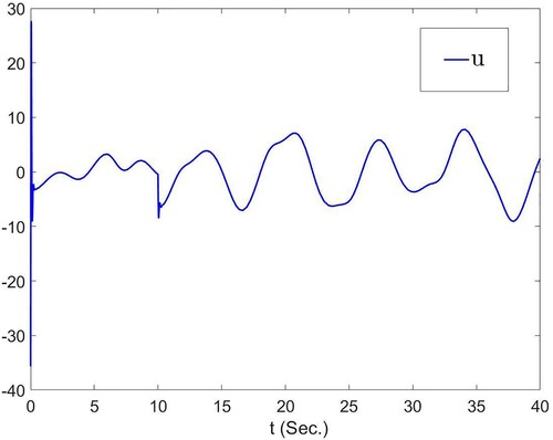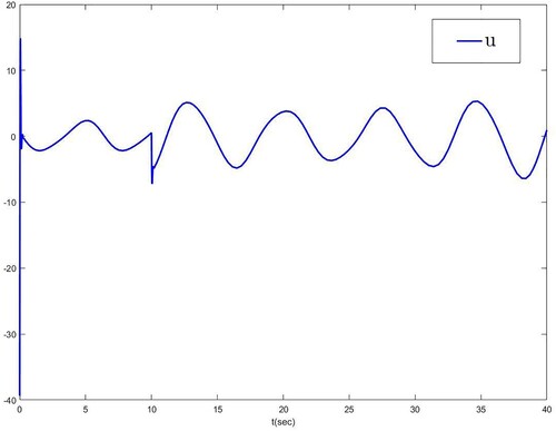Figures 4–6 display the curves of $||{\hat{\mathrm{\aleph }}}_{fi}||$, $||{\hat{\mathrm{\aleph }}}_{ci}||$ and $||{\hat{\mathrm{\aleph }}}_{fi}||$ where i = 1, 2, and the curves from these figures are decreasing. Figure 7 showcases the trajectory of optimal actual controller u. From the simulation results, the proposed scheme in this paper can achieve the desired control objective.

Figure 1. The trajectories of y, $y_r$ and $k_{1c}$.

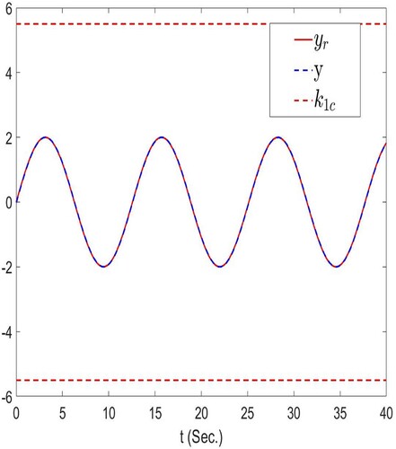
Figure 2. The trajectories of $z_1$ and $k_{1b}$.

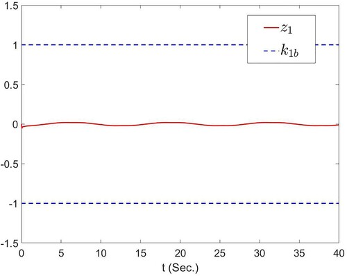
Figure 3. The trajectories of $x_2$ and $k_{2c}$.

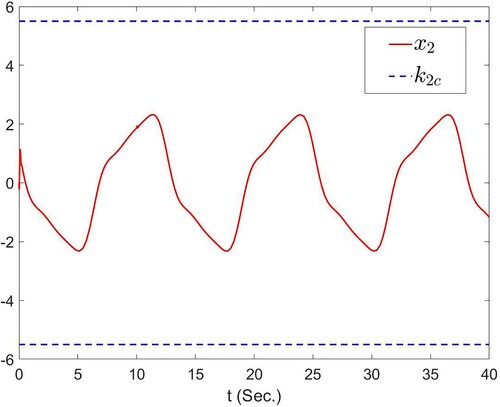
Figure 4. The curves of ${\hat{\mathrm{\aleph }}}_{c1}$ and ${\hat{\mathrm{\aleph }}}_{c2}$.

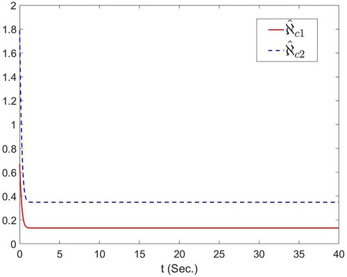
Figure 5. The curves of ${\hat{\mathrm{\aleph }}}_{a1}$ and ${\hat{\mathrm{\aleph }}}_{a2}$.

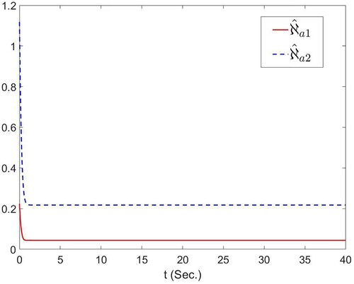
Figure 6. The curves of ${\hat{\mathrm{\aleph }}}_{f1}$ and ${\hat{\mathrm{\aleph }}}_{f2}$.

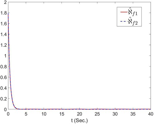
Figure 7. The trajectory of u.

Example 5.2

Similar to [9] and [48], this paper considers the robotic manipulator system as follows: (147) $J\ddot{S}+A\dot{S}+MGr\sin \left(S\right)=u\left(t\right),$(147) where S and $\dot{S}$ are the angle and angular velocity of the link, respectively, M is the total mass of the link, J is the rotational inertia of the motor, G is the gravitational acceleration, A is the damping coefficient. Assuming the effect of external disturbance and bias fault on the system is taken into account, (147(147) $J\ddot{S}+A\dot{S}+MGr\sin \left(S\right)=u\left(t\right),$(147) ) is rewritten as (148) $J\ddot{S}+A\dot{S}+MGr\sin \left(S\right)=u^A\left(t\right)+D\left(t\right).$(148) The parameter selection in (148(148) $J\ddot{S}+A\dot{S}+MGr\sin \left(S\right)=u^A\left(t\right)+D\left(t\right).$(148) ) is similar to that in [48], that is, $J=1,A=2,M=1,G=10,r=1$. Let $x_1=\dot{S}$, $x_2=\ddot{S}$ thus the system (147(147) $J\ddot{S}+A\dot{S}+MGr\sin \left(S\right)=u\left(t\right),$(147) ) can be rewritten as (149) $\begin{array}{r}\{\begin{array}{l}{\dot{x}}_1=x_1,\\ {\dot{x}}_2=u^A-10\sin \left(x_1\right)-2x_2+D\left(t\right),\end{array}\end{array}$(149) where $f_2\left({\overline{x}}_2\right)=-10\sin \left(x_1\right)-2x_2$, $u^A=u\left(t\right)+u_f$, the reference signal $y_r=0.2\sin \left(\mathrm{t}\right)$. The fuzzy logic system we used and bias fault signal are the same as in Example 5.1. The parameters used in the control strategy are designed as $m_1=m_2=2,{\gamma }_{c1}=6,{\gamma }_{a1}=4,{\gamma }_{c2}=15,{\gamma }_{a2}=13,k_{1c}=k_{2c}=5.5,k_{1b}=1,k_{2b}=2,{\sigma }_1={\sigma }_2=30,{\overline{\sigma }}_1={\overline{\sigma }}_2=10$ and $\delta =\frac{999}{1001}$. The reference trajectory $y_r$ and external disturbance $D\left(t\right)$ are defined as $y_r=0.2\sin \left(t\right)$ and $D\left(t\right)=0.3\sin \left(2t\right)$. The initial values are configured as ${\hat{\mathrm{\aleph }}}_{f1}\left(0\right)={\hat{\mathrm{\aleph }}}_{f2}\left(0\right)=[0.8,0.8,0.8,0.8,0.8{]}^T$, ${\hat{\mathrm{\aleph }}}_{c1}\left(0\right)=[0.2,0.1,0.1,0,0.1{]}^T$, ${\hat{\mathrm{\aleph }}}_{c2}\left(0\right)=[0.1,0,0,0.2,0.1{]}^T$, ${\hat{\mathrm{\aleph }}}_{a1}\left(0\right)=[0.1,0.2,0.1,0,0{]}^T$, ${\hat{\mathrm{\aleph }}}_{a2}\left(0\right)=[0.1,0,0,0.2,0.1{]}^T$, and $x_1\left(0\right)=x_2\left(0\right)=0$.

Figures 8–14 are the simulation results of the robotic manipulator system. Figure 8 demonstrates the trajectories of y, $y_r$ and $k_{1c}$, showing satisfactory control performance. As shown in Figure 9, the tracking error $z_1$ represented by the red solid line does not exceed the blue dashed line $k_{1b}$ and remains within a small neighbourhood relating to the origin. The trajectory of $x_2$, which does not cross the blue dashed line $k_{2c}$, is shown in Figure 10. Figures 11–13 display the curves of $||{\hat{\mathrm{\aleph }}}_{fi}||$, $||{\hat{\mathrm{\aleph }}}_{ci}||$ and $||{\hat{\mathrm{\aleph }}}_{fi}||$ where i = 1, 2. Figure 14 shows the trajectory of optimal actual controller u.

Figure 8. The trajectories of y, $y_r$ and $k_{1c}$.

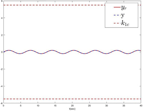
Figure 9. The trajectories of $z_1$ and $k_{1b}$.

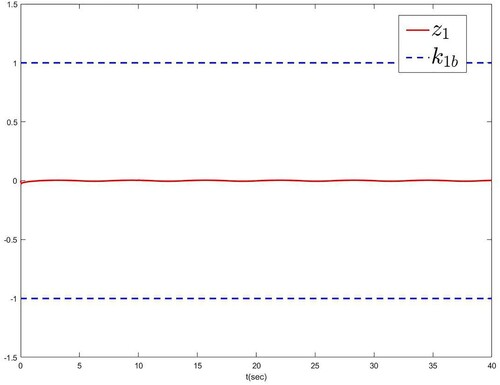
Figure 10. The trajectories of $x_2$ and $k_{2c}$.

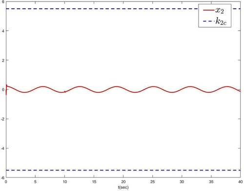
Figure 11. The curves of ${\hat{\mathrm{\aleph }}}_{c1}$ and ${\hat{\mathrm{\aleph }}}_{c2}$.

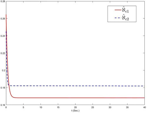
Figure 12. The curves of ${\hat{\mathrm{\aleph }}}_{a1}$ and ${\hat{\mathrm{\aleph }}}_{a2}$.

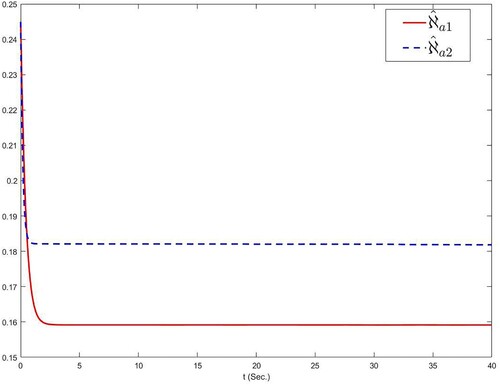
Figure 13. The curves of ${\hat{\mathrm{\aleph }}}_{f1}$ and ${\hat{\mathrm{\aleph }}}_{f2}$.

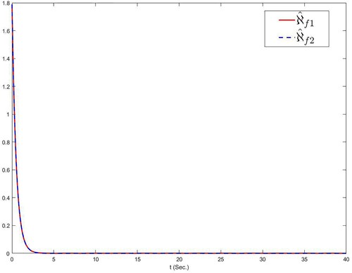
Figure 14. The trajectory of u.

6. Conclusion

In this article, the issue of adaptive fuzzy optimal finite-time control for uncertain nonlinear systems with bias fault and external disturbances is studied. Consider bias fault term and external disturbance as total disturbance, the disturbance observer is designed to track the total disturbance online, where the total disturbance consists of bias fault term and external disturbance. By combining with backstepping and ADP technologies, an adaptive fuzzy optimal finite-time control approach is proposed. It proves that all signals of closed-loop are finite-time stable, and the all system states in constrained sets. One future research direction is to extend the proposed method to more general systems such as stochastic systems [49], switched nonlinear systems [50,51] and uncertain under-actuated switched nonlinear systems [52]. In addition, it is another research direction to study unknown nonaffine nonlinear fault problems and unmodelled dynamics problems based on fixed time control [53–55].

Publisher's Note

Springer Nature remains neutral with regard to jurisdictional claims in published maps and institutional affiliations.

Acknowledgments

The authors thank the reviewers for their constructive comments in improving the quality of this paper. Zhidong Sun wrote the manuscript, Wei Gao and Li Liang revised and made improvements on the manuscript. The authors have worked equally when writing this paper. All authors read and approved the final manuscript.

Disclosure statement

No potential conflict of interest was reported by the author(s).

Data availability statement

Some or all data, models, or code generated or used during the study are available from the corresponding author by request.

Additional information

Funding

This work was supported by National Natural Science Foundation of China[12161094].

References

- Ma ZY, Ma HJ. Adaptive fuzzy backstepping dynamic surface control of strict-feedback fractional-order uncertain nonlinear systems. IEEE Trans Fuzzy Sys. 2020;28:122–133.
- Liang YJ, Li YX, Che WW, et al. Adaptive fuzzy asymptotic tracking for nonlinear systems with nonstrict-feedback structure. IEEE Trans Cybern. 2021;51:853–861.
- Ma H, Liang HJ, Zhou Q, et al. Adaptive dynamic surface control design for uncertain nonlinear strict-feedback systems with unknown control direction and disturbances. IEEE Trans Syst Man Cybern Syst. 2019;49:506–515.
- Wang HQ, Liu XP, Liu KF, et al. Approximation-based adaptive fuzzy tracking control for a class of nonstrict-feedback stochastic nonlinear time-delay systems. IEEE Trans Fuzzy Sys. 2015;23:1746–1760.
- Lai GY, Liu Z, Chen CLP, et al. Adaptive compensation for infinite number of time-varying actuator failures in fuzzy tracking control of uncertain nonlinear systems. IEEE Trans Fuzzy Sys. 2018;26:474–486.
- Zou AM, Hou ZG, Tan M. Adaptive control of a class of nonlinear pure-feedback systems using fuzzy backstepping approach. IEEE Trans Fuzzy Sys. 2008;16:886–897.
- Zhang HC, Song AG, Li HJ, et al. Novel adaptive finite-time control of teleoperation system with time-varying delays and input saturation. IEEE Trans Cybern. 2021;51:3724–3737.
- Bhat SP, Bernstein DS. Continuous finite-time stabilization of the translational and rotational double integrators. IEEE Trans Automat Contr. 1998;43:678–682.
- Qiu JB, Wang T, Sun KK, et al. Disturbance observer-based adaptive fuzzy control for strict-feedback nonlinear systems with finite-time prescribed performance. IEEE Trans Fuzzy Sys. 2022;30:1175–1184.
- Li Y, Qu F, Tong S. Observer-based fuzzy adaptive finite-time containment control of nonlinear multiagent systems with input delay. IEEE Trans Cybern. 2021;51:126–137.
- Zhang HG, Liu Y, Wang YC. Observer-based finite-time adaptive fuzzy control for nontriangular nonlinear systems with full-state constraints. IEEE Trans Cybern. 2021;51:1110–1120.
- Meng B, Liu WH, Qi XJ. Disturbance and state observer-based adaptive finite-time control for quantized nonlinear systems with unknown control directions. J Franklin Inst. 2022;359:2906–2931.
- Sui S, Chen CLP, Tong SC. Event-trigger-based finite-time fuzzy adaptive control for stochastic nonlinear system with unmodeled dynamics. IEEE Trans Fuzzy Sys. 2021;29:1914–1926.
- Saravanakumar R, Stojanovic SB, Radosavljevic DD, et al. Finite-time passivity-based stability criteria for delayed discrete-time neural networks via new weighted summation inequalities. IEEE Trans Neural Netw Learn Syst. 2019;30:58–71.
- Xia JW, Zhang J, Sun W, et al. Finite-time adaptive fuzzy control for nonlinear systems with full state constraints. IEEE Trans Syst Man Cybern. 2019;49:1541–1548.
- Wang YD, Zong GD, Yang D, et al. Finite-time adaptive tracking control for a class of nonstrict feedback nonlinear systems with full state constraints. Int J Robust Nonlinear Control. 2022;32:2551–2569.
- Zhao L, Liu GQ, Yu JP. Finite-time adaptive fuzzy tracking control for a class of nonlinear systems with full-state constraints. IEEE Trans Fuzzy Sys. 2021;29:2246–2255.
- Nguyen VT, Lin CY, Su SF, Sun W. Finite-time adaptive fuzzy tracking control design for parallel manipulators with unbounded uncertainties. Int J Fuzzy Syst. 2019;21:545–555.
- Wang LB, Wang HQ, Liu XP. Adaptive fuzzy finite-time control of stochastic nonlinear systems with actuator faults. Nonlinear Dyn. 2021;104:523–536.
- Bellman RE, Corporation R. Dynamic programming. Princeton (NJ): Princeton University Press; 1957.
- Werbos PJ. Approximate dynamic programming for real-Time control and neural modeling. Handb Intell Control Neural Fuzzy & Adapt Approaches. 1992;15:493–525.
- Abu-Khalaf M, Lewis FL. Nearly optimal control laws for nonlinear systems with saturating actuators using a neural network HJB approach. Automatica. 2005;41(5):779–791.
- Vamvoudakis KG, Lewis FL. Online actor-critic algorithm to solve the continuous-time infinite horizon optimal control problem. Automatica. 2010;46(5):878–888.
- Wen GX, Chen CLP, Feng J, et al. Optimized multi-agent formation control based on an identifier–actor–critic reinforcement learning algorithm. IEEE Trans Fuzzy Sys. 2018;26:2719–2731.
- Li KW, Li YM. Fuzzy adaptive optimal consensus fault-tolerant control for stochastic nonlinear multiagent systems. IEEE Trans Fuzzy Sys. 2022;30:2870–2885.
- Wen GX, Li B, Niu B. Optimized backstepping control using reinforcement learning of observer-critic-actor architecture based on fuzzy system for a class of nonlinear strict-feedback systems. IEEE Trans Fuzzy Sys. 2022;30:4322–4335.
- Lan J, Liu YJ, Yu DX, et al. Time-varying optimal formation control for second-order multiagent systems based on neural network observer and reinforcement learning. IEEE Trans Neural Netw Learn Syst. 2022. DOI:10.1109/TNNLS.2022.3158085
- Li YM, Liu YJ, Tong SC. Observer-based neuro-adaptive optimized control of strict-feedback nonlinear systems with state constraints. IEEE Trans Neural Netw Learn Syst. 2022;33:3131–3145.
- Bhasin S, Kamalapurkar R, Johnson M, et al. A novel actor–critic-identifier architecture for approximate optimal control of uncertain nonlinear systems. Automatica. 2013;49:82–92.
- Vamvoudakis KG, Miranda MF, Hespanha JP. Asymptotically stable adaptive-optimal control algorithm with saturating actuators and relaxed persistence of excitation. IEEE Trans Neural Netw Learn Syst. 2016;27:2386–2398.
- Zargarzadeh H, Dierks T, Jagannathan S. Optimal control of nonlinear continuous-time systems in strict-feedback form. IEEE Trans Neural Netw Learn Syst. 2015;26:2535–2549.
- Wen GX, Chen CLP, Ge SS. Simplified optimized backstepping control for a class of nonlinear strict-feedback systems with unknown dynamic functions. IEEE Trans Cybern. 2021;51:4567–4580.
- Zerari N, Chemachema M. Event-triggered adaptive output-feedback neural-networks control for saturated strict-feedback nonlinear systems in the presence of external disturbance. Nonlinear Dyn. 2021;104:1343–1362.
- Li HY, Zhao SY, He W, et al. Adaptive finite-time tracking control of full state constrained nonlinear systems with dead-zone. Automatica. 2019;100:99–107.
- Liu YC, Zhu QD, Wen GX. Adaptive tracking control for perturbed strict-feedback nonlinear systems based on optimized backstepping technique. IEEE Trans Neural Netw Learn. 2022;33:853–865.
- Sariyildiz E, Ohnishi K. On the explicit robust force control via disturbance observer. IEEE Trans Ind Electron. 2015;62:1581–1589.
- Tong SC, Li YM, Liu YJ. Observer-based adaptive neural networks control for large-scale interconnected systems with nonconstant control gains. IEEE Trans Neural Netw Learn Syst. 2021;32:1575–1585.
- Sun HB, Guo L. Neural network-based DOBC for a class of nonlinear systems with unmatched disturbances. IEEE Trans Neural Netw Learn Syst. 2017;28:482–489.
- Ji WY, Pan YN, Zhao M. Adaptive fault-tolerant optimized formation control for perturbed nonlinear multiagent systems. Int J Robust Nonlinear Control. 2022;32:3386–3407.
- Liu M, Ho DWC, Shi P. Adaptive fault-tolerant compensation control for Markovian jump systems with mismatched external disturbance. Automatica. 2015;58:5–14.
- Xu B, Shou YX, Luo J, et al. Neural learning control of strict-feedback systems using disturbance observer. IEEE Trans Neural Netw Learn. 2018;30:1296–1307.
- Song RZ, Lewis FL. Robust optimal control for a class of nonlinear systems with unknown disturbances based on disturbance observer and policy iteration. Neurocomputing. 2020;390:185–195.
- Zerari N, Chemachema M. Robust adaptive neural network prescribed performance control for uncertain CSTR system with input nonlinearities and external disturbance. Neural Comput Appl. 2020;32:10541–10554.
- Ran MP, Li JC, Xie LH. Reinforcement-learning-based disturbance rejection control for uncertain nonlinear systems. IEEE Trans Cybern. 2022;52:9621–9633.
- Chen M, Ge SS. Adaptive neural output feedback control of uncertain nonlinear systems with unknown hysteresis using disturbance observer. IEEE Trans Ind Electron. 2015;62:7706–7716.
- Li KW, Li YM. Adaptive NN optimal consensus fault-tolerant control for stochastic nonlinear multiagent systems. IEEE Trans Neural Netw Learn. 2023. 34(2):947–957. doi:10.1109/TNNLS.2021.3104839.
- Li HY, Wu Y, Chen M. Adaptive fault-tolerant tracking control for discrete-time multiagent systems via reinforcement learning algorithm. IEEE Trans Cybern. 2021;51:1163–1174.
- Xing LT, Wen CY, Liu ZT, et al. Adaptive compensation for actuator failures with event-triggered input. Automatica. 2017;85:129–136.
- Li YL, Liu B, Zong GD, et al. Command filter-based adaptive neural finite-time control for stochastic nonlinear systems with time-varying full state constraints and asymmetric input saturation. Int J Syst Sci. 2022;53:199–221.
- Zhang HY, Wang HQ, Niu B, et al. Sliding-mode surface-based adaptive actor-critic optimal control for switched nonlinear systems with average dwell time. Inf Sci. 2021;580:756–774.
- Wang HQ, Tong M, Zhao XD, et al. Predefined-time adaptive neural tracking control of switched nonlinear systems. IEEE Trans Cybern. 2022. DOI:10.1109/TCYB.2022.3204275
- Zhang HY, Zhao XD, Zhang L, et al. Observer-based adaptive fuzzy hierarchical sliding mode control of uncertain under-actuated switched nonlinear systems with input quantization. Int J Robust Nonlinear Control. 2022;32:8163–8185.
- Li YM, Sun KK, Tong SC. Observer-based adaptive fuzzy fault-tolerant optimal control for SISO nonlinear systems. IEEE Trans Cybern. 2019;49:649–661.
- Wang HQ, Xu K, Zhang HG. Adaptive finite-time tracking control of nonlinear systems with dynamics uncertainties. IEEE Trans Automat Contr. 2022. DOI:10.1109/TAC.2022.3226703
- Ma JW, Wang HQ, Qiao JF. Adaptive neural fixed-time tracking control for high-order nonlinear systems. IEEE Trans Neural Netw Learn. 2022. DOI:10.1109/TNNLS.2022.3176625