Information overflow between monetary policy transparency and inflation expectations using multivariate stochastic volatility models

Abstract

The forward-looking policy is useful for joint decision-making between public and monetary authorities. The study calculates the monetary policy transparency index, inflation expectations, and their volatility spillover effects at a data-driven angle. Optimization mechanisms of monetary policy transparency influencing inflation and inflation expectations volatility, and transparency index based on market participants’ optimization decisions are analysed. Multivariate stochastic volatility models for measuring the volatility of inflation and inflation expectations are analysed. Additionally, the relationships between inflation and inflation expectations volatility and transparency are tested empirically. Tests show that: first, the most suitable models for measuring volatility of inflation and inflation expectations are obtained. Second, monetary policy transparency has a negative effect on the volatility of inflation and inflation expectations. Third, there is a unidirectional Granger relationship from the volatility of inflation expectations to the volatility of inflation, and it indicates that the volatility of inflation expectations has an important guiding effect on that of inflation, and it is necessary to stabilize inflation expectations for stabilizing inflation. Fourth, improving monetary policy transparency can not only reduce inflation, inflation expectations, inflation volatility, inflation expectations volatility, but also reduce the sacrifice rate, that is, to stabilize the price level with less anti-inflation costs.

KEYWORDS:

• Forward-looking policy
• multivariate stochastic volatility model
• optimization mechanisms
• decision-making
• data-driven

MATHEMATICS SUBJECT CLASSIFICATIONS:

• 91B05
• 91B24
• 91B70

1. Introduction

With the development of information technology and data science, forward-looking policies, such as transparency policy and expectations management, show more and more important effects on public decision-making. The connection between public expectations and central bank policy is always a key issue in macroeconomic research fields, and monetary policy transparency is the link and indicator in the relation between forward-looking policy and expectations management. On the background that monetary authorities advocate achieving the coordination development of economic increase and price by macro-regulation models of pre-adjustment and minute adjustment, there are great theoretical and actual meanings for researching volatility information spillover effects of public inflation expectations, the dynamic changing situation of China’s monetary policy transparency, relationships among monetary policy transparency, inflation, inflation expectations, and sacrifice rate.

Existing literature mainly includes the following aspects: First, there is much literature on inflation expectations measurements and the relationship between inflation expectations and inflation. Inflation expectations are one kind of psychological feeling, essentially, it is always a hot and difficult issue in econometrics how to measure inflation expectations effectively.

There are five types of methods: the economic model method, the market information method, the model consistency expectations method, the survey questionnaire method, and the learning expectations method. The economic model method constructs an inflation prediction model that obtains the model’s regression coefficients using historical data, and then applies the obtained model to predict future inflation and takes the predicted values as public inflation expectations. The market information method deduces the implied public inflation expectations based on the relationships among some important economic variables or time structure in financial markets, and the method usually applies the interest rate term structure curve theory. The model consistency expectations method adds expectations into the model and supposes the public has rational expectations, and then deduces the implied expectations as being consistent with the model using the history data. The survey questionnaire method returns the essence of expectations to measure the public inflation expectations based on the public’s subjective judgment. The learning expectations method is one kind of extension of the economic model method, and the public constantly revises their judgment by the changes in economic situations and macro-policy information, namely, constantly adjusting expectations with the renewing information.

The above five kinds of methods have pros and cons. The economic model method is one kind of prediction method essentially, and it cannot reflect well public’s psychological factors. Their lack of interest rate data in the longer term due to China’s interest rate marketization is at the closing stage, and simultaneously China has not issued inflation-immunized bonds, and thus the application of market information method in China is limited to a certain degree. The model consistency expectations require relatively strong theoretical hypotheses. The survey questionnaire method reflects more intuitive changes in the public’s psychology, and the learning expectations method reflects better the formation process of the public’s expectations. Combining methods of the survey questionnaire and learning expectations, He et al. [1] proposed a predictable roll method that has a better prediction effect, does not need future information, and realized inflation expectations do not change with the information renewal. And thus as to inflation expectations measuring, a predictable roll method with the two characteristics of learning expectations and survey questionnaire is applied. In the future learning machines with rapid learning rates can be applied to inflation prediction and inflation expectations calculation [2].

The relationship between inflation expectations and inflation mostly focuses on researching the influence of inflation expectation on inflation using the Phillips curve. Zhang [3] researches the influences of inflation expectations and inflation persistence on inflation using the new Keynes-Phillips curve on the background of globalization. The results indicate that the two effects are almost equal. Fan and Gao [4] research the dynamic characteristics of China’s inflation using the hybrid new Keynes-Phillips curve and find that influencing directions of inflation persistence and inflation expectations on China’s inflation equilibrium is the same and inflation persistence plays a bigger effect than expectations.

Second, there is also much literature on the volatility of inflation and inflation expectations. Existing research mostly focuses on studying the volatility of inflation. Zhang and Zhang [5] test empirically periodic volatility characteristics of China’s inflation, and think that it is very important to rationally evaluate source shocks of China’s inflation volatility and that attention should be paid to gradualness in policy regulation. Because it is difficult to measure inflation expectations, the existing literature seldom studies the volatility of inflation expectations which has a micro-survey base. Wang and Wang [6] researched not only the relationship between expectations management and expectations volatility but also that between expectations management and bank risk-taking, but their inflation expectations are an extrapolation based on the sticky Phillips curve, and its essence is one kind of inflation prediction not considering public’s psychological feelings, and in addition, Wang and Wang [6] obtain volatility with the essence of one kind of periodic variation based on filtering. However, we measure volatility characteristics based on stochastic volatility models. Next, there is a great necessity for researching not only the volatility of inflation expectations but also spillover effects and inter-influences between the volatility of inflation and inflation expectations using modern econometric technologies.

Time-series data usually have the characteristics of volatility cluster, non-Gaussian distribution, etc., and GARCH models can portray these characteristics with simple modes. The variable’s conditional variance is the deterministic function of its past values in GARCH models, and this implies a latent hypothesis: horizontal process and volatility process of variable have a deterministic linkage, but it is difficult to be tested by theoretical or empirical studies, and the stochastic volatility model including latent stochastic factor, its volatility being influenced not only by variable but also by non-observable latent factor, is complex, but it can simulate data flexibly [7,8].

Although stochastic volatility has an attraction in theory, the latent volatility is added into the model by the nonlinear mode, and this leads to a likelihood function based on high-dimensional integration [9]. Yu and Meyer [10] propose several multi-variables stochastic volatility models such as multi-variables stochastic volatility models with the volatility Granger effect and that with dynamic correlation coefficient, and give empirical tests using weekly exchange rates data. On the one hand, financial decisions need to consider correlations and multi-variables stochastic volatility models display a very important effect on financial applications because asset pricing, risk measurement and management, asset allocation optimization, etc. all need to consider correlations between variables; on the other hand, the volatility of financial markets has a correlation with asset and time, and variables’ volatility is usually cross-markets and cross-assets, and thus multi-variables framework has higher statistical efficiency [8,10]. He et al. [11] investigated empirically volatility characteristics and Granger-spillover effects among different energy prices and expectations using the stochastic models. The paper applies multi-variables stochastic volatility models to measure the volatility of inflation and inflation expectations considering the following two reasons. Because stochastic volatility models have unobservable latent factors, they are superior to GARCH models. There is a volatility correlation between inflation and inflation expectations, and the correlation should be taken into consideration when making investment decisions.

Third, many scholars researched monetary policy transparency. Monetary policy transparency includes two aspects: one is the central bank information disclosure situation whether central banks release clear monetary policy information by corresponding channels. Two is the public understanding degree, even if central banks release clear monetary policy intentions, the public not understanding well indicates that monetary policy transparency is not high. Most of the existing research on monetary policy transparency focuses on the first aspect and the assignment value index method is applied usually. Chortareas et al. [12] research how monetary policy transparency influences inflation and inflation expectations and the relationship between transparency and an anti-inflationist, and they synthetically construct a transparency index based on four sub-projects being assigned from the angles of prediction and policy-making, and test the relationships among transparency, inflation, and sacrifice rate. Eijffinger and Geraats [13] consider five sub-projects: operations transparency, procedure transparency, economy transparency, policy transparency, and politics transparency based on information disclosure of monetary policymaking, the full score of every sub-projects being 3 points, and construct the monetary policy transparency index by adding assigning points of the five sub-projects. Van der Cruijsen et al. [14] researched the role of monetary policy transparency in reducing inflation persistence. Zhang et al. [15] researched the early relationship between china’s monetary policy transparency and anti-inflation, and china’s monetary policy transparency index from 1995 to 2008 is measured based on the assignment value index method which is easy to be applied but has relatively strong subjectivity and can not be applied to obtain time-series data.

Generally, the assignment value index method only reflects the first aspect of monetary policy transparency, namely, central bank information disclosure situations, and also many scholars are studying monetary policy transparency based on the changes in federal funds interest rates, and this method can not only reflect central bank information disclosure situations but also judge markets’ acceptance situations. Poole et al. [16] researched market participants’ expectations of Federal Reserve policy actions, and thought that an increase in monetary policy transparency is beneficial for market participants to forecast Federal Reserve policy actions and economic stability. As to the shortages of the traditional transparency index, based on market information, Kia [17] proposes a method for constructing a transparency index, which not only is dynamic and continuous and can provide time-series data to overcome the shortage of only doing cross-section studies, but also is a comprehensive index embodying central bank actions and public understanding degree, namely measuring both central bank information announcements and public understanding degree. Jia [18] constructs China’s monetary policy transparency index using China’s interbank overnight offered rates and bond repo rates and supposes that monetary policy transparency should be elevated in China by empirical tests. Sacrifice rate, which is a concept about monetary policy transparency, is usually applied to measure the anti-inflation cost and test the effect of monetary policy transparency. The same as Andersen and Wascher [19], if time t’s inflation is higher than that of the t–1 and t + 1, time t is defined as peak of inflation, and if time t’s inflation is lower than that of the t–1 and t + 1, time t is defined as the valley of inflation, and the term from peak to valley is defined as an anti-inflation period, and the sacrifice rate is defined as the ratio of cumulative variation of output gap to that of inflation in a anti-inflation period. The study explores also the relationship between China’s monetary policy transparency and sacrifice rate after constructing monetary policy transparency time-series data.

Van der Cruijsen et al. [14] researched the optimal monetary policy transparency, and thought that transparency increase in a certain degree is beneficial and of a certain degree will produce a negative effect making the public excessively dependent on information and the excessive information making the public confused. And then what is the situation of China’s monetary policy transparency? What are the influences of inflation, inflation expectations, inflation volatility, and inflation expectations volatility? The relationship between monetary policy transparency and sacrifice rate also needs to be studied deeply.

The study's core content encompasses the following aspects: Firstly, it examines the impact of national inflation, national inflation expectations, urban inflation, and urban inflation expectations on volatility through a comparative analysis with 18 diverse multi-variable stochastic volatility models. Secondly, it rigorously examines the effects of monetary policy transparency on inflation, inflation expectations, inflation volatility, and inflation expectations volatility from various perspectives. Thirdly, it conducts a comprehensive verification of the influence exerted by inflation expectations on inflation, considering multiple vantage points.

The study’s structure is arranged as follows: The second part is mechanism analysis. The mechanism of monetary policy transparency influencing the volatility of inflation expectations is discussed. The third part is China’s monetary policy transparency index construction. The fourth part introduces multi-variables stochastic volatility models and gives volatility measurements of inflation and inflation expectations. The fifth part tested empirically volatility spillover effects between inflation and inflation expectations, respectively. The sixth part tested the relationships between monetary policy transparency and China’s anti-inflation cost. The seventh part is the conclusions.

2. Optimization mechanism analysis of monetary policy transparency influencing inflation expectations volatility

Kydland and Prescott [20] summarized the relationship between employment rate deviation and the bias of inflation and inflation expectations by models, and based on the model spirit, Geraats [21], Chortareas et al. [12] analysed the incentive effect of monetary policy transparency based on the overall supply curve:$ga{p}_t-ga{p}^{\mathrm{\Delta }}=\omega (cp{i}_t-cp{i}_t^e)+{\xi }_t$,$ga{p}_t$ and $ga{p}^{\mathrm{\Delta }}$ represent actual and natural output rates, $cp{i}_t$ and $cp{i}_t^e$ represent real and expected inflation rates, respectively, and ${\xi }_t$ is the residual error. The central bank determines the objectives of output and inflation by $max\{-(ga{p}_t-ga{p}^a{)}^2-\mu (cp{i}_t-cp{i}^a{)}^2\}$ where $ga{p}^a$ and $cp{i}^a$ represent targeted output and targeted inflation, respectively, and simultaneously ascertain monetary increasing rate $i_t$ by $i_t=cp{i}_t+\chi {\xi }_t-{\zeta }_t$ where $\chi$ indicates the response of an individual to economic structure bias and ${\zeta }_t$ is the speed error. Chortareas et al. [12] obtained the following by deducting (1) $\begin{array}{r}cpi=\left(\frac{\omega }{\mu }\right)v-\left(\frac{{\omega }^2}{{\omega }^2+\mu }\right)\left(\frac{\omega }{\mu }\right){\xi }^{f,p}+(\varphi -{\varphi }^{f,cb})+(\chi -\frac{\omega }{\mu +{\omega }^2}){\xi }^{f,cb}-\chi \xi \end{array}$(1) ${\xi }^{f,p}$ and ${\xi }^{f,cb}$ are the prediction biases of the public and central bank, respectively, in contrast to the public, the central bank has information advantages, and Peek et al. [22] think that the Federal Reserve Commission has information advantages that have not only statistical significance but also significant economic meaning, and they can enhance the prediction accuracy of inflation. In economics, transparency mainly indicates information symmetry and judgments of a central bank and the public on the economic structure both have uncertainty in monetary policy fields. Generally, the central bank has information advantages and can judge more precisely, and the public gives prediction based on the central bank’s judgment and its special analysis, and thus the public prediction includes two parts: one is on the central bank prediction, and the other is the part which the individual having uniquely, and transparency reflects information asymmetry degree of central bank and the public, and the higher transparency corresponds to the larger weight of central bank prediction and the smaller weight of individual characteristics when the individual makes prediction [12,21], and by dividing public’s prediction bias into two parts: ${\xi }^{f,p}=\rho {\xi }^{f,cb}+(1-\rho )\vartheta$, the following formulation can be obtained: (2) $\begin{array}{r}\begin{array}{l}cpi-cp{i}^e=\left(1-{\displaystyle \frac{{\omega }^2}{{\omega }^2+\mu }}\right)\left({\displaystyle \frac{\omega }{\mu }}\right){\xi }^{f,p}+(\varphi -{\varphi }^{f,cb})\\ +(\chi -{\displaystyle \frac{\omega }{\mu +{\omega }^2}}){\xi }^{f,cb}-\chi \xi \\ ={\displaystyle \frac{\omega }{{\omega }^2+\mu }}(\rho {\xi }^{f,cb}+(1-\rho )\vartheta )+(\varphi -{\varphi }^{f,cb})+(\chi -{\displaystyle \frac{\omega }{\mu +{\omega }^2}}){\xi }^{f,cb}-\chi \xi \\ ={\displaystyle \frac{\omega }{{\omega }^2+\mu }}\rho {\xi }^{f,cb}+{\displaystyle \frac{\omega }{{\omega }^2+\mu }}(1-\rho )\vartheta +(\varphi -{\varphi }^{f,cb})+(\chi -{\displaystyle \frac{\omega }{\mu +{\omega }^2}}){\xi }^{f,cb}-\chi \xi \\ ={\displaystyle \frac{\omega }{{\omega }^2+\mu }}(\rho -1){\xi }^{f,cb}+{\displaystyle \frac{\omega }{{\omega }^2+\mu }}(1-\rho )\vartheta +(\varphi -{\varphi }^{f,cb})+\chi ({\xi }^{f,cb}-\xi )\\ ={\displaystyle \frac{\omega }{{\omega }^2+\mu }}(\rho -1)({\xi }^{f,cb}-\vartheta )+(\varphi -{\varphi }^{f,cb})+\chi ({\xi }^{f,cb}-\xi )\end{array}\end{array}$(2) Chortareas et al. [12] additionally consider the variance of inflation deviating from its target value, and supposing its target value is 0, the second-order differentiation indicates that if $2\rho {\sigma }_{{\xi }^{f,cb}}^2<v+{\sigma }_{{\xi }^{f,p}}^2$, and then $\frac{\mathrm{\partial }E{(cpi)}^2}{\mathrm{\partial }\rho }<0$, and this indicates that the higher transparency corresponds to the lower inflation expectations volatility under certain conditions, and this demonstrates theoretically the relationship between monetary policy transparency and inflation expectations volatility.

Based on Chortareas et al. [12], Zhang et al. [15] obtain the following formula by deduction and simplifying inflation constitution: (3) $\begin{array}{r}cpi=\left(\frac{\omega }{\mu }\right)v-\left(\frac{{\omega }^2}{{\omega }^2+\mu }\right)\left(\frac{\omega }{\mu }\right){\xi }^{f,p}+(\varphi -{\varphi }^{f,cb})-\frac{\omega }{\mu +{\omega }^2}{\xi }^{f,cb}\end{array}$(3) Zhang et al. [15] indicate that by derivation, when ${\sigma }_{{\xi }^{f,p}}^2-{\sigma }_{{\xi }^{f,cb}}^2<(1-\rho {)}^2(\vartheta -\nu {)}^2$, $\frac{\mathrm{\partial }E{(cpi)}^2}{\mathrm{\partial }\rho }<0$, and this indicates that there is a reverse relationship between inflation expectations volatility and transparency.

The importance of monetary policy transparency in the effective execution of monetary policy has been recognized gradually since the 1990s [23]. Some scholars expound on the effect of public information on individual decisions from other angles. Monetary policy transparency increase can not only strengthen the trust of the public in policy, and thus let the public inflation expectations be consistent with policy quickly, but also decrease the public information asymmetry and eliminate low efficiency caused by the public conceptual persistence, and thus decrease the sacrifice rate of anti-inflation cost [24].

Transparency is beneficial to strengthen trust, and trust is the key to monetary policy efficient execution, trust rooted in transparency is the strong medium for maintaining monetary value [25]. An increase in transparency can reduce information asymmetry in the private sector, and transparency has the effect of restraining and smoothing volatility of economic growth through information advantages [26]. These research studies indicate that monetary policy transparency may have an important effect on public inflation, inflation expectations, inflation volatility, and inflation expectations volatility from angles of information transmission etc. The following hypotheses can be obtained, based on the above analyses:

Hypothesis 1: Monetary policy transparency has inverse relationships with public inflation and inflation expectations.

Hypothesis 2: Monetary policy transparency has inverse relationships with public inflation volatility and inflation expectations volatility.

Chortareas et al. [12] tested empirically the reverse relationship between inflation and transparency based on cross-section data from different countries. The corresponding empirical research of Zhang et al. [15] mainly tested the relationship between inflation and transparency, and they only calculated China’s transparency total index is 3, and then qualitatively judged the relationship between China’s transparency situation variation and anti-inflation cost. The paper calculates time-series data of China transparency, inflation expectations, inflation volatility and inflation expectations volatility, and to enhance the robustness we simultaneously give empirical tests on the situations of first order and second order, which respectively correspond to the relationship between inflation or inflation expectations and monetary policy transparency, and that between inflation volatility or inflation expectations volatility and monetary policy transparency. We analyse not only the relationship between inflation or inflation expectations and transparency but also that between inflation volatility or inflation expectations volatility and transparency.

3. Construction of China’s monetary policy transparency index based on market participants’ optimization decision

Trends of different interest rates are determined by joint decision-making between central banks and market participants, and the transparency index can be obtained based on financial big data. To research dynamic relationships between inflation expectations volatility or inflation volatility and transparency, time-series data of monetary policy transparency must be obtained, and thus China’s monetary policy transparency index is constructed based on China’s actual data by applying the time-series method using interest rate market data, as shown in Figure 1.

Figure 1. Dynamic changing trend of China’s monetary policy transparency.

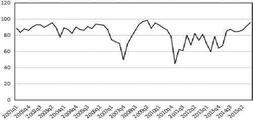
Transparency has two meanings: First, based on the angle of the central bank, the transparency reflects the central bank disclosing situations on related regimes, measures, and attitudes. Second, based on the public angle, transparency reflects understanding situations at the public level, namely, the public’s understanding degree and reflection on information published by the central bank. And thus transparency index construction includes mainly two categories: One is based on qualitative judgement and scoring, and the other returns the transparency index’s essence that using financial markets’ final understanding degree and effect on central bank information, and explores whether the impact of an important event on market can be transmitted to market participants quickly by choosing important event day. The second kind of transparency index is not only time-series data which can reflect dynamic variation situations of monetary policy transparency, but also a comprehensive index that reflects central bank’s disclosure situations, the public’s understanding and final actual actions based on their optimization decision.

Generally, the traditional method of monetary policy transparency construction can only obtain data of non-time-series form, and they can only be mainly applied to cross-section and static analyses due to the limit of data number.

As to the shortage of traditional measuring methods of monetary policy transparency, Kia [17] proposes a dynamic method of transparency index construction based on time-series data, which mainly constructs a transparency index based on market participants’ understanding degree of meeting decisions of Federal Open Market Committee (FOMC), and decisions, out of meeting, concerning target variations. The concrete steps are as follows:

First, event date selections. Poole et al. [16] and Kia [17] take the meeting date of FOMC, whether the target interest rate changes, or the day when deciding the target interest rate variation between FOMC meeting dates, as the event date and the next day is taken as event date if FOMC meeting date is during weekend or holiday. Because the interest rate target mechanism has not been implemented in China, similar to Jia [18], the event date is determined by the mode of a major event. Monetary policy major events, mainly deposits and loans interest rate adjustment, reserve ratio adjustment, monetary policy committee meeting, and central bank monetary policy execution report publication, etc., which may arouse monetary market interest rate changes, have been chosen according to monetary policy memorabilia every quarterly published in the website of People's Bank of China, and the day these major events happening is determined as event date (demarcation point), and if the day major events happening is not the trading day, it is substituted by the nearest trading day around it.

Second, the credit risk premium bias is calculated by the following formulas. (4) $\begin{array}{r}\begin{array}{rl}D{R}_t& =IO{R}_t-TB{R}_t\\ MD{R}_t& ={\sum }_{k=1}^{l}D{R}_{t-k}/m\\ E_t& =|D{R}_t-MD{R}_t|\end{array}\end{array}$(4) where IORt and TBRt indicate inter-bank offered rate (IOR) and treasury bill rate (TBR) respectively, and $D{R}_t$ measures the risk premium between credit risk and term structure risk, namely, credit risk premium, and $MD{R}_t$ indicates the mean of credit risk premiums ($D{R}_t$) around two event days, and $t-l$ and $m$ indicate the last event day and the trading days since the last event day [17,18]. Under the hypothesis that the public has not expected significant variations of relevant inter-bank risk or government credibility to debt unless monetary authorities take action or other shocks bring the asymmetric changes of the two interest rates, $Di{f}_t$ will not deviate its long mean level [17]. Many scholars [17,27] think that $D{R}_t$ may be an indicator of monetary policy standpoint, and it includes much information on future variations of real macro-economic variables. Kia [17] indicates empirically that the deviation of $D{R}_t$ and its mean level is decided by market participant actions, and these actions are mainly based on their expectations of federal future policies. The deviation is temporary if the monetary policy transparency is high, and the deviation is non-temporary if he monetary policy transparency is low because market participants may misjudge the central bank’s intentions and take actions opposite to the central bank’s expectations, and thus central bank should take more measures to rectify it [17].

Third, the monetary policy transparency index can be obtained by bias indexation using the following formula. (5) $\begin{array}{r}TI=100/\exp (E_t)\end{array}$(5)

When the central bank takes tight policy by selling treasury bills to raise the benchmark interest rate, an increase in commercial banks’ funding needs in the inter-bank market makes the federal fund rate $FF{R}_t$ rise and $D{R}_t$ rise also, simultaneously to make up for liquidity, commercial banks sell also treasury bills in monetary market and treasury bill rate $TBR$ rises also and thus $D{R}_t$ inclines to equilibrium, and the deviation of $D{R}_t$ and its equalization value depends on central bank monetary policy transparency and generally there is a reverse relationship between them: the deviation is low when the transparency is high and high deviation with low transparency [17].

Kia [17] calculates monetary policy transparency indexes based on Equation (5), the range of the index is from 0 to 100, if $E_t=0$, namely, there is no bias between $D{R}_t$ and its equalization value $TI=100$ and this indicates that monetary policy is completely transparent, and if $E_t=12$, $TI=\text{0}\text{.0006 }$ approximating to 0, and this indicates that monetary policy is complete non-transparent.

Fourth, it is extended to non-event days, additionally, and the specific algorithm is similar to that of event days. China’s monetary policy transparency index is calculated using the data of inter-bank offered 1-day weighting interest rates, and inter-bank repo 7-day weighting interest rates. Figure 1 indicates the dynamic changing characteristics of the index and it can be seen that China’s monetary policy transparency index has an increased trend since 2011.

China’s monetary policy transparency was relatively high and steady from the first quarter of 2001 to the fourth quarter of 2006, and it dropped greatly during 2007 and reached its partial lowest point in the fourth quarter of 2007. This may be about America’s subprime mortgage crisis. Because America’s subprime mortgage crisis in 2007 had an impact on China, problems such as price rise and fall etc. appeared in China, and a series of targeting policies were taken by the central bank, this may bring a large fluctuation of monetary policy transparency. The second stage when China’s monetary policy transparency fluctuated greatly during 2011, which was exactly Europe’s financial crisis eruption time, China takes also a series of targeting policies to cope with the international financial crisis, and this causes the relatively great fluctuation of China’s monetary policy transparency. The persistent enhancement of China’s monetary policy transparency corresponds to the fact that China government pays more attention to expectations management, forward-looking regulation mode, and pre-tuning and fine-tuning strategies. Simultaneously, the term that monetary policy transparency decreasing largely corresponds exactly to the term inflation being at a relatively high level, and this indicates that monetary policy transparency has a reverse relationship with inflation level and the enhancement of monetary policy transparency is beneficial to reducing inflation level.

4. Volatility measurements of inflation and inflation expectations

On the one hand, the public form their own inflation expectations based on the past trends of inflation, other macroeconomic variables and own experience, on the other hand, the public inflation expectations include much information and also have an inverse effect on inflation, and thus keeping inflation expectations steady is an important method to keep price steady. There is a great need to study deeply the difference between volatility characteristics of inflation and inflation expectations, and the volatility information spillover effects between them using econometric methods. Next, we apply multivariate stochastic volatility models with dynamic correlation coefficients to test empirically volatility characteristics of inflation and inflation expectations, and volatility spillover effects between them.

To measure the relationships between the volatility of inflation and inflation expectations, and monetary policy transparency, first of all, it is needed to calculate the volatility of inflation and inflation expectations. The study applies a binary stochastic volatility model to measuring the volatility of inflation and inflation expectations because a single variable stochastic volatility model cannot measure effectively the dynamic relationship between two variables. The following 9 binary stochastic volatility models are constructed based on Yu and Meyer [10]: (6) $\begin{array}{rl}\left(\begin{array}{c}cp{i}_t\\ cp{i}_t^e\end{array}\right)& =diag(\exp ({\theta }_t/2))\left(\begin{array}{c}{\xi }_{1t}\\ {\xi }_{2t}\end{array}\right),\left(\begin{array}{c}{\xi }_{1t}\\ {\xi }_{2t}\end{array}\right)\sim \sim N(0,{\mathrm{\Sigma }}_{\xi ,t}=\left(\begin{array}{cc}1& {\lambda }_t\\ {\lambda }_t& 1\end{array}\right)),\\ \left(\begin{array}{c}{\theta }_{cpi,t+1}\\ {\theta }_{cp{i}^e,t+1}\end{array}\right)& =\left(\begin{array}{c}{\alpha }_{cpi}\\ {\alpha }_{cp{i}^e}\end{array}\right)+diag\left(\begin{array}{cc}{\phi }_{11}& {\phi }_{12}\\ {\phi }_{21}& {\phi }_{22}\end{array}\right)\left(\left(\begin{array}{c}{\theta }_{cpi,t}\\ {\theta }_{cp{i}^e,t}\end{array}\right)-\left(\begin{array}{c}{\alpha }_{cpi}\\ {\alpha }_{cp{i}^e}\end{array}\right)\right)\\ & +\left(\begin{array}{c}{\varsigma }_{cpi,t}\\ {\varsigma }_{cp{i}^e,t}\end{array}\right),\left(\begin{array}{c}{\varsigma }_{cpi,t}\\ {\varsigma }_{cp{i}^e,t}\end{array}\right)\sim N(0,diag({\sigma }_{{\varsigma }_{cpi}}^2,{\sigma }_{{\varsigma }_{cp{i}^e}}^2))\end{array}$(6)

1. If ${\phi }_{12}={\phi }_{21}=0,{\lambda }_t=0$, then it is the basic model, and written as model 1, and its essence is the combination of the two single variable stochastic volatility models.

2. If ${\phi }_{12}={\phi }_{21}=0,{\lambda }_t=\lambda$, then it is the constant correlation binary stochastic volatility model, and written as model 2.

3. If ${\phi }_{12}={\phi }_{21}=0,{\lambda }_t=\frac{\exp (b_t)-1}{\exp (b_t)+1},b_{t+1}={\beta }_0+\psi (b_t-{\beta }_0)+{\sigma }_{\lambda }{\vartheta }_t,{\vartheta }_t\sim N(0,1)$, then it is the dynamic correlation binary stochastic volatility model, and written as model 3.

4. If ${\phi }_{12}=0,{\phi }_{21}\ne 0,{\lambda }_{\text{t}}=\lambda$ or ${\phi }_{12}\ne 0,{\phi }_{21}=0,{\lambda }_{\text{t}}=\lambda$, then it is the constant correlation binary stochastic volatility model with the unidirectional Granger effect, and written as model 4. There are two situations for model 4 by variables order during specific application: volatility spill-over effects from inflation expectations to inflation, and inflation to inflation expectations, represented as model 4a and 4b, respectively.

5. If ${\phi }_{12}=0,{\phi }_{21}\ne 0,{\lambda }_t=\frac{\exp (b_t)-1}{\exp (b_t)+1},b_{t+1}={\beta }_0+\beta (b_t-{\beta }_0)+{\sigma }_{\lambda }{\vartheta }_t,\vartheta \sim N(0,1)$ or ${\phi }_{12}\ne 0,{\phi }_{21}=0,{\lambda }_t=\frac{\exp (b_t)-1}{\exp (b_t)+1},b_{t+1}={\beta }_0+\beta (b_t-{\beta }_0)+{\sigma }_{\lambda }{\vartheta }_t,{\vartheta }_t\sim N(0,1)$, then it is the dynamic correlation binary stochastic volatility model with the unidirectional Granger effect, and written as model 5. Similar to model 4, in concrete applications, model 5 also is divided into two: model 5a and 5b.

6. If ${\phi }_{12}\ne 0,{\phi }_{21}\ne 0,{\lambda }_{\text{t}}=\lambda$, then it is the constant correlation binary stochastic volatility model with the bidirectional Granger effect, and written as model 6.

7. If ${\phi }_{12}\ne 0,{\phi }_{21}\ne 0,{\lambda }_t=\frac{\exp (b_t)-1}{\exp (b_t)+1},b_{t+1}={\beta }_0+\beta (b_t-{\beta }_0)+{\sigma }_{\lambda }{\vartheta }_t,{\vartheta }_t\sim N(0,1)$, then it is the dynamic correlation binary stochastic volatility model with the bidirectional Granger effect, and written as model 7.

In addition, financial time series often have characteristics of a thick tail, the above 9 models are also extended from normal distribution to t distribution to test the effects of various models at different distributions.

Supposing $\alpha$ is the parameter, and $\theta$ is the logarithm latent variance, and letting $\delta =(\alpha ,\theta )$, and then the posterior distribution is as follows: (7) $\begin{array}{r}p(\delta /(cpi,cp{i}^e))={\int }_{{\theta }_1}\cdots {\int }_{{\theta }_T}p(\delta ,{\theta }_1,\cdots ,{\theta }_T)d{\theta }_T\cdots d{\theta }_1\end{array}$(7)

Conditional covariance of the multivariate GARCH model at time t can be calculated using information until time t–1, but as for that of the multivariate stochastic volatility model, because of including latent factors, it is needed to calculate by the integration of united likelihood function, and thus likelihood function of multivariate stochastic volatility model does not have the form of closed set, and it is not easy to obtain the exact max likelihood value [8].

The general integration simulation technology is a relatively good method to solve integration problems, but as for high dimensional integration, generally, it is difficult to be fulfilled by directly independent sampling, and Liesenfeld and Richard [9] think that likelihood function based on high dimensional integration is the difficulty in estimating the stochastic volatility model, and apply the effectively key sampling method based on the Monte Carlo technology to solve the evaluation problem of high dimensional integration, and Durham [7] also thinks that the Monte Carlo technology can solve the evaluation problem of high dimensional integration, and the MCMC method can sample effectively by constructing Markov chains to solve the above problem [10].

DIC criterion is a relatively good standard to judge the good and bad stochastic volatility models. In the classical model construction field, model evaluation is mainly based on the comprehensive consideration of fitting effectiveness, model complexity and parameter freedom degree, and based on AIC and BIC information criteria, Spiegelhalter et al. [28] proposed the DIC criterion which is the Bayes simulation of AIC and has a similar theory base with AIC, but the broader application scope and can be applied to evaluating a complex model, for example, a comparing model whose parameter number is not defined clearly.

Inflation expectations are calculated by survey data. Empirical tests are given based on data on national and urban inflation rates, respectively. To guarantee model estimating effects, we apply the double chains to estimate parameters, elaborately design initial parameter values, give a de-fire simulation of 10,000 times, run 90,000 times again, and finally give the posterior test result of the latter 90,000 times. As for stochastic models, ensuring parameter convergence is important for guaranteeing the effectiveness of parameter estimation, and convergence judgement figures of 9 models under t distribution are given in the example ${\varphi }_{12}$.

Table 1 shows the main estimated parameter results of 9 models under normal distribution based on national inflation rates, and Table 2 shows those under t distribution. Data in tables are estimated parameter values at mean level, 5% quantile and 10% quantile, respectively.

Table 1. Estimated parameter results and effects of 9 models under normal distribution based on national inflation rates.

Estimated parameter	Model 1	Model 2	Model 3	Model 4a	Model 4b	Model 5a	Model 5b	Model 6	Model 7
${\alpha }_{\text{c}}$	1.307;	1.36;	1.331;	1.255;	1.42;	1.319;	1.5;	1.381;	1.429;
	0.4822;	0.7852;	0.7435;	0.5812;	0.8692;	0.6196;	0.9491;	0.7436;	0.7444;
	0.6768	0.9299	0.8922	0.7203	1.027	0.7777	1.086	0.8836	0.9056
${\alpha }_{\text{e}}$	0.673;	0.7042;	0.6599;	0.6623;	0.6438;	0.7489;	0.7161;	0.7021;	0.7511;
	0.0734;	0.3025;	0.2624;	0.3007;	0.1283;	0.3725;	0.2249;	0.297;	0.3752;
	0.2408	0.3924	0.3564	0.382	0.2526	0.4536	0.3356	0.377	0.4569
${\beta }_{\text{cc}}$	0.9312;	0.9278;	0.9274;	0.7898;	0.8987;	0.8141;	0.9054;	0.8086;	0.795;
	0.8292;	0.804;	0.8034;	0.5527;	0.6949;	0.5834;	0.7134;	0.5593;	0.5478;
	0.8631	0.8498	0.8488	0.6178	0.7669	0.6463	0.785	0.6317	0.6185
${\beta }_{\text{ee}}$	0.8893;	0.8546;	0.8575;	0.8587;	0.7939;	0.8538;	0.7941;	0.8389;	0.8322;
	0.7192;	0.6447;	0.6486;	0.6629;	0.5414;	0.6434;	0.5506;	0.6036;	0.5949;
	0.7762	0.7089	0.7129	0.7225	0.6156	0.7078	0.6182	0.6736	0.6655
${\beta }_{\text{ce}}$				1.069;		0.8379;		0.7088;	0.8138;
				0.2402;		−		−	0.0314;
				0.395		0.7308;		0.6648;	0.1456
						−0.2434		−0.107
${\beta }_{\text{ec}}$					0.2218;		0.1963;	−0.007;	−0.0183;
					−0.7716;		−0.4734;	−0.2728;	−0.317;
					−0.2012		−0.1095	−0.161	−0.1362
$\chi$			0.8585;			0.855;	0.8586;		0.8517;
			0.6515;			0.6415;	0.6516;		0.6371;
			0.7154			0.7071	0.7139		0.7017
$\rho$		0.7855;	0.7833;	0.7678;	0.7699;	0.7983;	0.7892;	0.7708;	0.7875;
		0.6915;	0.6668;	0.6605;	0.6689;	0.6641;	0.6641;	0.6668;	0.6686;
		0.7162	0.6997	0.6894	0.6962	0.7052	0.7015	0.6942	0.7036
DIC	459.885	414.115	413.18	408.411	415.415	410.302	414.138	411.353	410.265

Table 2. Estimated parameter results and effects of 9 models under t distribution based on national inflation rates.

Estimated parameter	Model 1	Model 2	Model 3	Model 4a	Model 4b	Model 5a	Model 5b	Model 6	Model 7
${\alpha }_{\text{c}}$	1.202;	1.181;	1.256;	1.105;	1.312;	1.13;	1.307;	1.416;	1.313;
	0.417;	0.6027;	0.7148;	0.3835;	0.8432;	0.3863;	0.8156;	0.5611;	0.6506;
	0.6133	0.7572	0.8493	0.5535	0.9393	0.5594	0.9429	0.7584	0.8122
${\alpha }_{\text{e}}$	0.5296;	0.4703;	0.5526;	0.4569;	0.5347;	0.4778;	0.5317;	0.6362;	0.5614;
	−0.0005;	0.0583;	0.1406;	0.0042;	0.0074;	0.0967;	0.0146;	0.136;	0.0862;
	0.1252	0.1539	0.2331	0.1229	0.1214	0.1813	0.1246	0.2416	0.1968
${\beta }_{\text{cc}}$	0.9265;	0.9149;	0.9156;	0.7922;	0.8752;	0.7994;	0.8906;	0.8104;	0.8168;
	0.8077;	0.7572;	0.7686;	0.5333;	0.6471;	0.5445;	0.6769;	0.5588;	0.5781;
	0.8503	0.8166	0.8219	0.6116	0.722	0.6129	0.7506	0.6287	0.6428
${\beta }_{\text{ee}}$	0.8872;	0.8602;	0.8511;	0.8779;	0.7959;	0.8608;	0.7936;	0.8475;	0.8406;
	0.7079;	0.6516;	0.6326;	0.6854;	0.5492;	0.6577;	0.5495;	0.6241;	0.6038;
	0.7671	0.7161	0.6995	0.7471	0.6181	0.7203	0.6146	0.6908	0.6757
${\beta }_{\text{ce}}$				0.9066;		0.9426;		0.6216;	0.6427;
				0.0236;		−0.6785;		−0.0825;	−0.296;
				0.2676		0.1856		0.1064	0.0157
${\beta }_{\text{ec}}$					0.1274;		0.2543;	0.0051;	−0.0739;
					−1.212;		−0.4232;	−0.2317;	−0.6149;
					−0.5507		−0.1632	−0.0796	−0.3731
$\chi$			0.8644;			0.8565;	0.8619;		0.8595;
			0.6592;			0.643;	0.6504;		0.6487;
			0.722			0.7097	0.7153		0.7135
$\rho$		0.7815;	0.8031;	0.773;	0.7782;	0.7748;	0.7775;	0.7819;	0.7871;
		0.6831;	0.6929;	0.6645;	0.6731;	0.6407;	0.6404;	0.6755;	0.6544;
		0.7094	0.7252	0.6936	0.7012	0.68	0.6767	0.705	0.6931
$\tau$		9.595;	9.831;	10.18;	9.801;	10.22;	9.724;	10.29;	10.29;
		4.744;	4.852;	5.016;	4.794;	5.116;	4.828;	5.135;	4.987;
		5.45	5.593	5.785	5.528	5.88	5.532	5.907	5.757
DIC	466.576	348.145	351.357	340.131	351.305	345.438	348.337	345.472	350.021

First, the order of various model effects is as follows: The best is model 4a, the constant correlation binary stochastic volatility model with the unidirectional Granger effect, measuring the volatility spillover effect of inflation expectations on inflation, and the second place is model 7, the dynamic correlation binary stochastic volatility model with the bidirectional Granger effect, and the third place is model 5a, the dynamic correlation binary stochastic volatility model with the unidirectional Granger effect, measuring the volatility spillover effect of inflation expectations on inflation, and the worst is model 1, the basic stochastic model which is the simple combination of the two single variable stochastic models, and these indicate whether the correlation coefficient or the Granger effect can enhance model prediction effects. Second, except for model 1, the effect differences among the other models are not large, and the size and direction of coefficients are also basically consistent. Third, the effect of model 1 is the worst, and its estimating effect is largely inferior to the other 8 models, this indicates that the two independent stochastic volatility models cannot measure effectively the volatility of inflation and inflation expectations, and it is needed that taking the two as a whole to measure volatility spillover effects between them. Fourth, the volatility of inflation is larger than that of inflation expectations, and the persistence of inflation volatility is also larger than that of inflation expectations volatility. Fifth, there is an information spillover effect from the volatility of inflation expectations to that of inflation. As to models with unidirectional spillover effect, the model measuring the spillover volatility effect of inflation expectations on inflation is superior to that measuring the volatility spillover effect of inflation on inflation expectations; and as to the best models: model 4a and model 7, volatility spillover coefficients of inflation expectation on inflation are all positive at the form of mean, 5% , media, and 95% quantile levels. Sixth, there is no volatility spillover effect of inflation on inflation expectations. Model 2 is superior to model 4b, and model 3 is superior to model 5b, and these indicate that whether constant or dynamic correlation coefficient multivariate stochastic volatility models being introduced volatility spillover effect of inflation on inflation expectations, model effects cannot be enhanced, As to the four models including the volatility spillover effect of inflation on inflation expectations: model 4b, model 5b, model 6, and model 7, volatility spillover coefficients β ec of inflation on inflation expectations are non-significant in the first two models, and they are even significantly negative in the latter two models and this is not per theory and reality. Comprehensively, we argue that the volatility spillover coefficient of inflation on inflation expectations is non-significant. This indicates mainly volatility spillover from inflation expectations to inflation between them, and thus it is very important to ensure the stability of inflation expectations volatility.

Due to the lack of priori test methods on operation length, some statistics are needed to be calculated to judge convergence [29]. Gelman and Rubin [30] offer methods on how to judge parameter convergence in iterative simulation. Brooks and Gelman [29] give extension and pictorial methods.

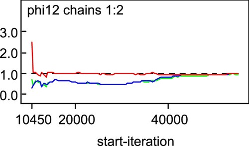
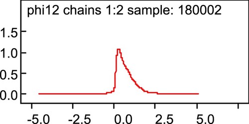
β ce in model 7 is taken as an example to indicate the estimating effect of the parameter. In Figure 2, β ce overlaps each other in double chains, and the gap in double chains is relatively small, this indicates that β ce is convergent. In Figure 3, β ce overlaps each other in double chains, and the gap in double chains is relatively small, this indicates that β ce is convergent. In Figure 4, there is a maximum value in probabilities of β ce equalling different values, and this indicates not only that β ce is convergent but also that β ce equals the abscissa value corresponding to the maximum value point at a relatively large probability.

Figure 2. Changing trends of β ce at double chains.

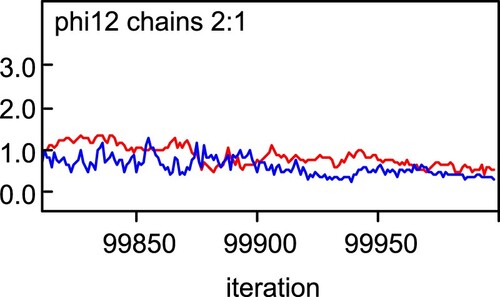
Figure 3. Changing trends of β ce at double chains.

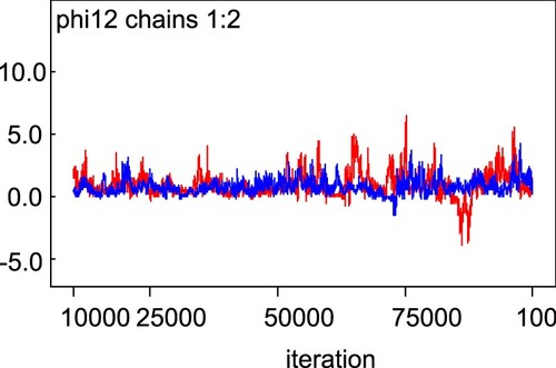
Figure 4. Probabilities of β ce values.

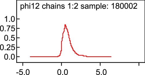
Brooks and Gelman [29] provide a pictorial method to judge parameter convergence, and as shown in Figure 5, the Gelman-Rubin test value of β ce is close to 1, and this also indicates that β ce is convergent. Overall, Figures 2 and 5 indicate that β ce is convergent, and the estimation is effective, and these indicate that the method applied by the manuscript is effective, and can measure effectively the volatile characteristics of inflation and inflation expectations and their spillover effects.

Figure 5. The Gelman-Rubin test of β ce.

First, the order of various model effects is as follows: The best is model 4a, the constant correlation binary stochastic volatility model with the unidirectional Granger effect, measuring the volatility spillover effect of inflation expectations on inflation. The second place is model 5a, the dynamic correlation binary stochastic volatility model with the unidirectional Granger effect, measuring the volatility spillover effect of inflation expectations on inflation, and the third place is model 6, the constant correlation binary stochastic volatility model with the bidirectional Granger effect. The worst is model 1, the basic stochastic model which is the simple combination of the two single variable stochastic models, and these indicate whether correlation coefficient or the Granger effect can both enhance model prediction effects. Second, except for model 1, the effect differences among the other models are not large, and the size and direction of coefficients are also basically consistent. Third, the effect of model 1 is the worst, and its estimating effect is largely inferior to the other 8 models, this indicates that the two independent stochastic volatility models cannot measure effectively the volatility of inflation and inflation expectations, and it is needed that taking the two as a whole to measure volatility spillover effects between them. Fourth, the volatility of inflation is larger than that of inflation expectations, and the persistence of inflation volatility is also larger than that of inflation expectations volatility. Fifth, there is an information spillover effect from the volatility of inflation expectations to that of inflation. As to models with unidirectional spillover effect, the model measuring the spillover volatility effect of inflation expectations on inflation is superior to that measuring the volatility spillover effect of inflation on inflation expectations; and as to the best models: model 4a, volatility spillover coefficients of inflation expectation on inflation are all positive at the form of mean, 5% , media, and 95% quantile levels. Sixth, there is no volatility spillover effect of inflation on inflation expectations. As to the four models including the volatility spillover effect of inflation on inflation expectations: model 4b, model 5b, model 6, and model 7, volatility spillover coefficients β ec of inflation on inflation expectations are non-significant in the first three models, and it is even significantly negative in model 7 and this is not in accordance with theory and reality. Comprehensively, we argue that the volatility spillover coefficient of inflation on inflation expectations is non-significant. This indicates mainly volatility spillover from inflation expectations to inflation between them, and thus it is very important to ensure the stability of inflation expectations volatility.

The t distribution is superior to the normal distribution for all the models except for model 1, and simultaneously, parameter τ of the t distribution is all about 10 at various models, and these indicate that the t distribution is superior to the Normal distribution. Among all 18 models measuring volatility characteristics of national inflation expectations and inflation, according to the DIC criterion, the best is model 4a at t distribution, and thus it is applied to measure the volatility characteristics of inflation expectations and inflation.

The volatility spillover effect of inflation expectations on inflation is concerned mostly with, the estimated density distribution map of β ce of four models including the coefficient is supplied.

Figures 6–9 indicate that β ce at different models only has one extreme point, and the abscissa of the extreme point is bigger than 0, and these indicate that β ce is convergent and positive at a high probability. These are consistent with the former conclusion and indicate that there is a significant spillover effect of inflation expectation volatility on inflation volatility, and stabilizing inflation expectation volatility is needed to keep inflation volatility steady. Similarly, estimated parameter results of various models based on urban inflation rates are obtained, as shown in Table 3.

Figure 6. Probabilities of β ce values in model 4a.

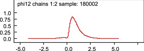
Figure 7. Probabilities of β ce values in model 5a.

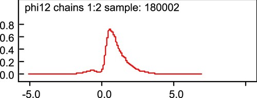
Figure 8. Probabilities of β ce values in model 6.

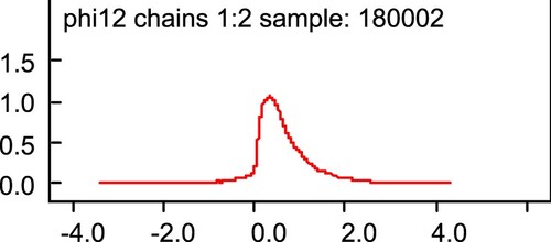
Figure 9. Probabilities of β ce values in model 7.

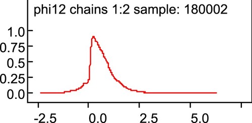
Table 3. Estimated parameter results and effects of 9 models under normal distribution based on urban inflation rates.

Estimated parameter	Model 1	Model 2	Model 3	Model 4a	Model 4b	Model 5a	Model 5b	Model 6	Model 7
${\alpha }_{\text{c}}$	1.246;	1.323;	1.38;	1.273;	1.409;	1.303;	1.397;	1.355;	1.41;
	0.3467;	0.7011;	0.7967;	0.551;	0.87;	0.5935;	0.8139;	0.6824;	0.7013;
	0.5548	0.8506	0.9389	0.6908	1.011	0.7393	0.9637	0.8324	0.8584
${\alpha }_{\text{e}}$	0.575;	0.6292;	0.6762;	0.6005;	0.6091;	0.6387;	0.6187;	0.6327;	0.6652;
	−0.018;	0.2124;	0.2909;	0.2563;	0.1184;	0.2935;	0.0637;	0.2534;	0.2442;
	0.1434	0.3127	0.3734	0.3268	0.2278	0.3745	0.1882	0.3335	0.3241
${\beta }_{\text{cc}}$	0.9367;	0.9329;	0.926;	0.7821;	0.9055;	0.787;	0.9196;	0.8111;	0.8043;
	0.8427;	0.8185;	0.7972;	0.5409;	0.7111;	0.5409;	0.7589;	0.5781;	0.5587;
	0.8732	0.8609	0.8449	0.6108	0.7828	0.6107	0.8215	0.6391	0.6207
${\beta }_{\text{ee}}$	0.8916;	0.8565;	0.8517;	0.8659;	0.7913;	0.8619;	0.7985;	0.8512;	0.8488
	0.7213;	0.6509;	0.6421;	0.6666;	0.5414;	0.6687;	0.5612;	0.6291;	0.6307;
	0.7785	0.7146	0.7054	0.729	0.6123	0.7272	0.6291	0.6973	0.696
${\beta }_{\text{ce}}$				1.194;		0.9796;		0.6396;	0.646;
				0.3298;		−1.066;		−0.696;	−0.7568;
				0.467		−0.4644		−0.3592	−0.3341
${\beta }_{\text{ec}}$					0.1668;		0.2034;	0.0009;	−0.0288;
					−0.8006;		−0.2263;	−0.2053;	−0.3393;
					−0.1654		−0.0289	−0.1234	−0.1995
$\chi$			0.8555;			0.8531;	0.8532;		0.8545;
			0.6444;			0.6449;	0.6403;		0.6444;
			0.7089			0.7075	0.7035		0.7081
$\rho$		0.7935;	0.8104;	0.7693;	0.778;	0.7832;	0.7785;	0.779;	0.7916;
		0.6998;	0.7012;	0.6638;	0.6784;	0.6501;	0.6539;	0.6742;	0.661;
		0.7248	0.7303	0.6919	0.7052	0.6902	0.688	0.7023	0.6949
DIC	448.612	402.801	403.529	395.686	404.095	396.77	403.195	398.66	399.767

First, the order of various model effects is as follows: The best is model 4a, the constant correlation binary stochastic volatility model with the unidirectional Granger effect, measuring the volatility spillover effect of inflation expectations on inflation. The second place is model 5a, the dynamic correlation binary stochastic volatility model with the unidirectional Granger effect, measuring the volatility spillover effect of inflation expectations on inflation. The third place is model 6, the constant correlation binary stochastic volatility model with the bidirectional Granger effect. The worst is model 1, the basic stochastic model which is the simple combination of the two single variable stochastic models, and these indicate whether correlation coefficient or the Granger effect can enhance model prediction effects. Second, except for model 1, the effect differences among the other models are not large, and the size and direction of coefficients are also basically consistent. Third, the effect of model 1 is the worst, and its estimating effect is largely inferior to the other 8 models, this indicates that the two independent stochastic volatility models cannot measure effectively the volatility of inflation and inflation expectations, and it is needed that taking the two as a whole to measure volatility spillover effects between them. Fourth, the volatility of inflation is larger than that of inflation expectations, and the persistence of inflation volatility is also larger than that of inflation expectations volatility. Fifth, there is an information spillover effect from the volatility of inflation expectations to that of inflation. As to models with unidirectional spillover effect, the model measuring the spillover volatility effect of inflation expectations on inflation is superior to that measuring the volatility spillover effect of inflation on inflation expectations. As to the best model: model 4a, the volatility spillover coefficient of inflation expectation on inflation is all positive in the form of mean, 5% , media, and 95% quartile levels. Sixth, there is no volatility spillover effect of inflation on inflation expectations. As to the four models including the volatility spillover effect of inflation on inflation expectations: model 4b, model 5b, model 6, and model 7, volatility spillover coefficients β ec of inflation on inflation expectations are non-significant in the first three models, and it is even significantly negative in model 7 and this is not in accordance with theory and reality. Comprehensively, we argue that the volatility spillover coefficient of inflation on inflation expectations is non-significant. This indicates that there exists mainly volatility spillover from inflation expectations to inflation between them, and thus it is very important to ensure the stability of inflation expectations volatility.

Model 4a, model 5a, model 6, and model 7 include volatility spillover effects of inflation expectations on inflation, and the estimated density distribution maps of β ce in four models are supplied as follows.

Figures 10–13 indicate that β ce at different models only has one extreme point, and the abscissa of the extreme point is bigger than 0, and these indicate that β ce is convergent and positive at a high probability. These are consistent with the former conclusion and indicate that there is a significant spillover effect of inflation expectation volatility on inflation volatility, and stabilizing inflation expectation volatility is needed to keep inflation volatility steady. The same as national inflation rates, the model residual distribution is also extended from normal distribution to t distribution, and estimated parameter results of various models at t distribution are obtained, as shown in Table 4.

Figure 10. Probabilities of β ce values in model 4a.

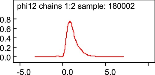
Figure 11. Probabilities of β ce values in model 5a.

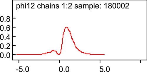
Figure 12. Probabilities of β ce values in model 6.

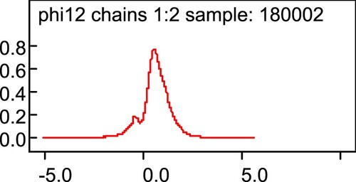
Figure 13. Probabilities of β ce values in model 7.

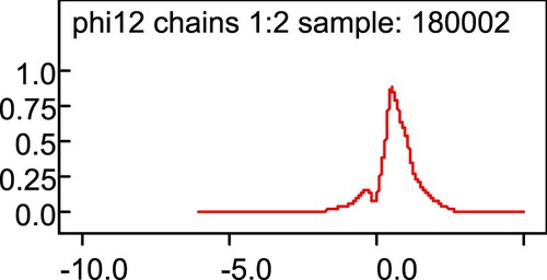
Table 4. Estimated parameter results and effects of 9 models under t distribution based on urban inflation rates.

Estimated parameter	Model 1	Model 2	Model 3	Model 4a	Model 4b	Model 5a	Model 5b	Model 6	Model 7
${\alpha }_{\text{c}}$	1.147;	1.21;	1.194;	1.152;	1.309;	1.213;	1.32;	1.359;	1.365;
	0.261;	0.6121;	0.607;	0.4362;	0.7817;	0.4632;	0.7615;	0.6045;	0.6;
	0.4742	0.7621	0.7494	0.5978	0.9016	0.644	0.8968	0.752	0.7657
${\alpha }_{\text{e}}$	0.4492;	0.4547;	0.4465;	0.4092;	0.4924;	0.4821;	0.4956;	0.5102;	0.5394;
	−0.072;	0.0157;	0.0183;	0.0246;	−0.0455;	0.0227;	−0.0498;	0.0916;	0.0754;
	0.0535	0.1219	0.1105	0.092	0.0695	0.1386	0.0641	0.1763	0.1737
${\beta }_{\text{cc}}$	0.9348;	0.918;	0.923;	0.7989;	0.901;	0.8092;	0.9096;	0.8038;	0.8072;
	0.834;	0.7709;	0.789;	0.5713;	0.6951;	0.5711;	0.7294;	0.5552;	0.5511;
	0.8683	0.8254	0.8389	0.6267	0.7696	0.6363	0.7958	0.6254	0.6261
${\beta }_{\text{ee}}$	0.8878;	0.857;	0.8526;	0.8702;	0.7966;	0.8762;	0.794;	0.8439;	0.8462;
	0.7068	0.6503;	0.6399;	0.6603;	0.5478;	0.6849;	0.5481;	0.612;	0.62;
	;0.7662	0.7122	0.7047	0.7273	0.6161	0.7442	0.6183	0.6824	0.6887
${\beta }_{\text{ce}}$				0.9573;		0.9097;		0.7921;	0.7114;
				−1.029;		−0.2766;		0.002;	0.0861;
				0.2112		0.26		0.1446	0.1602
${\beta }_{\text{ec}}$					0.0836;		0.204;	0.0475;	0.0278;
					−0.9794;		−0.2583;	−0.0717;	−0.1868;
					−0.346		−0.0848	−0.0431	−0.0711
$\chi$			0.8564;			0.854;	0.8589;		0.854;
			0.6462;			0.6419;	0.6507;		0.6424;
			0.7106			0.7068	0.714		0.7065
$\rho$		0.7962;	0.8;	0.7736;				0.7813;	0.7849;
		0.6989;	0.68;	0.6677;				0.6772;	0.6531;
		0.7253	0.7135	0.6954				0.7054	0.6908
$\tau$	10.9;	10.02;	9.998;	10.39;	10.11;	10.54;	9.924;	10.3;	10.23;
	5.515;	4.852;	4.929;	5.224;	4.962;	5.31;	4.822;	5.184;	5.105;
	6.328	5.641	5.668	6.005	5.744	6.11	5.58	5.957	5.877
DIC	455.982	334.353	340.518	330.884	339.796	330.072	338.346	331.996	330.537

First, the order of various model effects is as follows. The best is model 5a, the dynamic correlation binary stochastic volatility model with the unidirectional Granger effect, measuring the volatility spillover effect of inflation expectations on inflation. The second place is model 7, the dynamic correlation binary stochastic volatility model with the bidirectional Granger effect. The third place is model 4a, the constant correlation binary stochastic volatility model with the unidirectional Granger effect, measuring the volatility spillover effect of inflation expectations on inflation. The worst is model 1, the basic stochastic model which is the simple combination of the two single variable stochastic models, and these indicate that whether correlation coefficient or Granger effect can enhance model prediction effects. Second, except for model 1, the effect differences among the other models are not large, and the size and direction of coefficients are also basically consistent. Third, the effect of model 1 is the worst, and its estimating effect is largely inferior to the other 8 models, this indicates that the two independent stochastic volatility models cannot measure effectively the volatility of inflation and inflation expectations, and it is needed that taking the two as a whole to measure volatility spillover effects between them. Fourth, the volatility of inflation is larger than that of inflation expectations, and the persistence of inflation volatility is also larger than that of inflation expectations volatility. Fifth, there is an information spillover effect from the volatility of inflation expectations to that of inflation. As to models with the unidirectional spillover effect, the model measuring the spillover volatility effect of inflation expectations on inflation is superior to that measuring the volatility spillover effect of inflation on inflation expectations; and as to the four models: model 4a, model 5a, model 6, and model 7, including the volatility spillover effects of inflation expectations on inflation, the coefficients are all positive at the form of mean, 10% , media, and 95% quartile levels. Sixth, there is no volatility spillover effect of inflation on inflation expectations. As to the four models including the volatility spillover effect of inflation on inflation expectations: model 4b, model 5b, model 6, and model 7, volatility spillover coefficients of β ec of inflation on inflation expectations are non-significant. This indicates that there exists mainly volatility spillover from inflation expectations to inflation between them, and thus it is very important to ensure the stability of inflation expectations volatility.

As to t distribution and Normal distribution, except for the basic model 1, t distribution is superior to Normal distribution in the other models, and in the meantime, the parameter τ of t distribution in the model is all about 10, and these indicate that t distribution is superior to Normal distribution. Among 18 models measuring volatility characteristics of urban inflation expectations and inflation, the best model is model 5a under t distribution by the DIC criterion, thus model 5a is applied to measuring volatility characteristics of inflation expectations and inflation. Probability figures of β ce which measure the volatility spillover effect of inflation expectations on inflation, in model 4a, model 5a, model 6, and model 7 are also supplied as follows.

Figures 14–17 all indicate that β ce, which measures the volatility spillover effect of inflation expectations on inflation, is convergent, and positive at a high probability, and these are consistent with the front conclusions and indicate that inflation expectations have a significant spillover effect on inflation.

Figure 14. Probabilities of β ce values in model 4a.

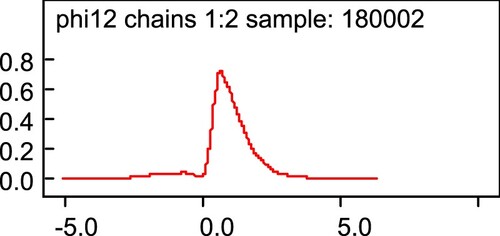
Figure 15. Probabilities of β ce values in model 5a.

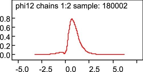
Figure 16. Probabilities of β ce values in model 6.

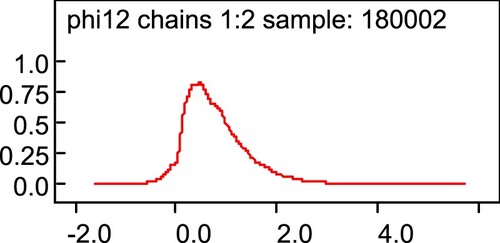
Figure 17. Probabilities of β ce values in model 7.

Among 18 models measuring volatility characteristics of national inflation expectations and inflation, the best model is model 4a under t distribution by DIC criterion, and thus model 4a is applied to measuring volatility characteristics of national inflation expectations and inflation. Among 18 models measuring volatility characteristics of urban inflation expectations and inflation, the best model is model 5a under t distribution by the DIC criterion, and thus model 5a is applied to measuring volatility characteristics of urban inflation expectations and inflation.

5. Inflation expectations volatility and monetary policy transparency

To strengthen the test effect, we also consider inflation volatility when testing empirically the relationship between inflation expectations volatility and monetary policy transparency. The relationships among inflation volatility, inflation expectations volatility, and monetary policy transparency are measured and to strengthen test result robustness, those among inflation, inflation expectations, and monetary policy transparency are measured additionally.

5.1. Inflation volatility, inflation expectations volatility, and monetary policy transparency

There are two angles for the front inflation expectations: national perspective and urban perspective, and we study empirically from national and urban perspectives.

5.1.1. Research based on national perspective

The Granger causality test is carried out first, and the driving relations among inflation volatility, inflation expectations volatility, and transparency are tested from the econometric angle. Because the test result of Granger causality is very sensitive to lagged term selection, choosing carefully lagged terms based on the VAR model is needed. The max-lagged term is 8 considering quarterly data being applied, and the best-lagged term is 3 by LR and HQ criteria, and test results are shown in Table 5.

Table 5. Granger causality test results of inflation volatility, inflation expectations volatility, and transparency.

Hypothesis H0	F-statistic and p-value
Inflation expectations volatility is not Granger’ s cause of transparency	0.2173 (0.8839)
Transparency is not Granger’ s cause of inflation expectations volatility	2.8374 (0.0473)
Inflation volatility is not Granger’ s cause of transparency	0.8319 (0.4827)
Transparency is not Granger’ s cause of inflation volatility	1.1861 (0.3245)
Inflation volatility is not Granger’ s cause of inflation expectations volatility	0.0595 (0.9807)
Inflation expectations volatility is not Granger’ s cause of inflation volatility	49.9918 (4* 10^− 15)

As shown in Table 5, there exists a one-way Granger causality effect from monetary policy transparency to inflation expectations volatility between them; there does not exist a Granger causality effect between inflation volatility and monetary policy transparency, and there exists a one-way Granger causality effect from inflation expectations volatility to inflation volatility between them. These indicate that there may exist a dynamic relationship between monetary policy transparency to inflation expectations volatility, and inflation volatility among the three variables, and this is consistent with former theoretical analyses and empirical tests. Thus structural VAR model is built by the order of monetary policy transparency, inflation expectations volatility, and inflation volatility.

The VAR model proposed by Sims [31] transforms large-scale macro-models into unrestricted and simplified forms by taking all the variables as endogenous variables, VAR models have the advantage of not needing to discriminate the explained and explaining variables but they also have disadvantages of lacking economic theory support and being incapable of measuring contemporaneous relationships among variables. Bernanke [32] changes the form of the VAR model proposed by Sims [31], and the basic economy structure perturbation items are obtained by VAR model residuals orthogonalization to reflect latent economy structure influence. Structural VAR models overcome the disadvantages of VAR models and include both the advantages of the structural model and the VAR model. Structural VAR models include contemporaneous variables and there are many parameters to be estimated, and thus certain restraints need to be imposed to transform them to VAR models of reduced form to estimate corresponding parameters, and there are 3 restrained forms of C, K, and AB, and the form of AB is applied in this paper. (8) $\begin{array}{r}A=\left(\begin{array}{ccc}1& a_{12}& a_{13}\\ a_{21}& 1& a_{23}\\ a_{31}& a_{32}& 1\end{array}\right),B=\left(\begin{array}{ccc}NA& 0& 0\\ 0& NA& 0\\ 0& 0& NA\end{array}\right)\end{array}$(8)

Three restrained conditions are still needed for such a form of AB. Generally, the responses of inflation expectations and inflation on monetary policy transparency have some lag, and there are no contemporaneous impacts, and thus we let a₁₂ =  0, a₁₃ =  0; and as indicated by the former empirical results, there is volatility spillover effect of inflation expectations on inflation between them, and thus we suppose that there no contemporaneous impact of inflation volatility on inflation expectations volatility, namely, a₂₃ = 0.

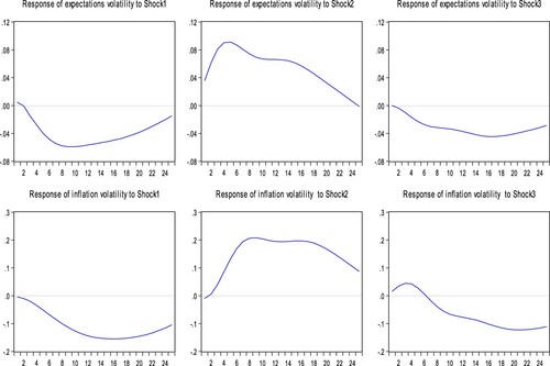
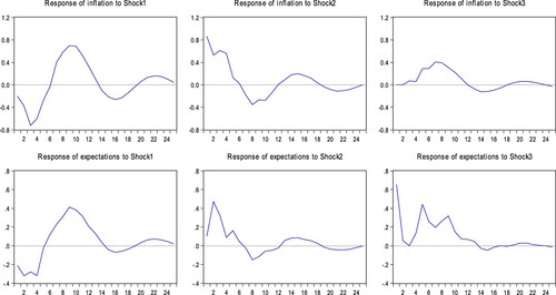
As shown in Figure 18, first, transparency has a negative effect on the volatility of inflation expectations and inflation, and a transparency increase corresponds to a volatility decrease in inflation expectations and inflation. Second, inflation expectations volatility has a positive effect on inflation volatility, and inflation expectations volatility increase corresponds to inflation volatility increase.

Figure 18. Structural impulse responses of inflation volatility, inflation expectations volatility and transparency.

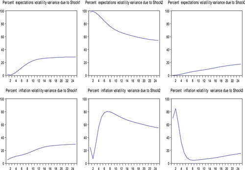
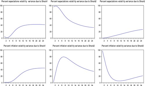
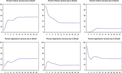
As shown in Figure 19, first, inflation expectations volatility is influenced mostly by itself, and transparency secondly, and inflation volatility minimally. Second, inflation volatility is influenced mostly by inflation expectations volatility, and transparency secondly, and itself minimally In the beginning it is influenced mostly by itself, but after the fourth period, the effect of inflation expectations volatility is larger than that of inflation volatility, and after the sixth period, the effect of transparency is also larger than that of inflation volatility, and this is in consistence with the former conclusion: ‘ inflation expectations has a large effect on inflation’ . Seen from a relatively long period, whether inflation volatility or inflation expectations volatility are influenced mostly by inflation expectations volatility mostly, and monetary policy transparency secondly, and thus keeping inflation expectations steady, and strengthening monetary policy transparency are needed to stabilize effectively inflation.

Figure 19 . Structural variance decomposition of inflation volatility, inflation expectations volatility and transparency.

5.1.2. Research based on urban perspective

Driving relationships among inflation volatility, inflation expectations volatility, and transparency are tested empirically by Granger causality. The lagged term is chosen carefully based on the VAR model because the testing result of Granger causality is very sensitive to lagged terms. The max lagged term is 8 considering quarterly data are applied, and the best lagged term is selected as 2 by the criteria of LR and HQ, and testing results are shown in Table 6.

Table 6. Granger causality testing results of inflation volatility, inflation expectations volatility, and transparency.

Hypothesis H0	F-statistic and p-value
Inflation expectations volatility is not Granger’ s cause of transparency	0.3662 (0.6951)
Transparency is not Granger’ s cause of inflation expectations volatility	5.2142 (0.0086)
Inflation volatility is not Granger’ s cause of transparency	0.50219 (0.6081)
Transparency is not Granger’ s cause of inflation volatility	0.72762 (0.4878)
Inflation volatility is not Granger’ s cause of inflation expectations volatility	0.26724 (0.7665)
Inflation expectations volatility is not Granger’ s cause of inflation volatility	35.5515 (2* 10^− 10)

In Table 6, there exists a one-way Granger causality effect from monetary policy transparency to inflation expectations volatility between them; there does not exist a Granger causality effect between inflation volatility and monetary policy transparency, and there exists a one-way Granger causality effect from inflation expectations volatility to inflation volatility between them. These indicate that there may exist a dynamic relationship between monetary policy transparency inflation expectations volatility, and inflation volatility among the three variables, and this is consistent with former theoretical analyses and empirical tests. Thus a structural VAR model is built by the order of monetary policy transparency, inflation expectations volatility, and inflation volatility.

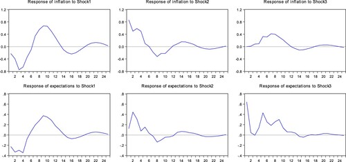
According to Figure 20, first, monetary policy transparency has a negative effect on the volatility of inflation expectations and inflation, and transparency increase can decrease the volatility of inflation expectations and inflation. Second, inflation expectations volatility has a positive effect on inflation volatility, and thus controlling inflation volatility needs controlling inflation expectations volatility.

Figure 20. Impulse responses of inflation volatility, inflation expectations volatility and transparency.

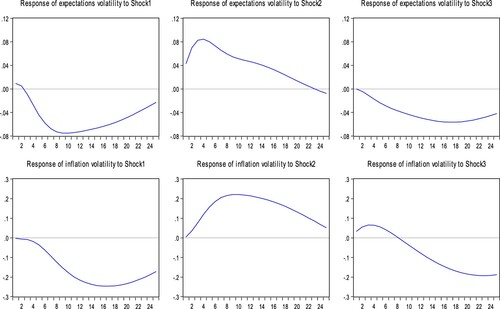
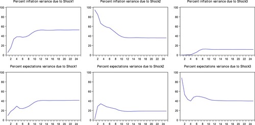
According to Figure 21, first, inflation expectations volatility is influenced mostly by itself early, but it is influenced increasingly by transparency over time, and after a long period it is influenced mostly by transparency, and least by inflation volatility. Second, the influencing effect of inflation volatility on itself falls fast with time, and its effect is less than that of inflation expectations volatility after the fourth period, that of transparency after the eighth period, and in the long run, transparency has the biggest effect, followed by expectations volatility, and inflation volatility the least. Seen from a relatively long period, whether inflation volatility or inflation expectations volatility is mostly influenced by monetary policy transparency , and thus in the long run strengthening monetary policy transparency is needed to stabilize effectively inflation volatility and inflation expectations volatility.

Figure 21. Variance decomposition of inflation volatility, inflation expectations volatility and transparency.

5.2. Inflation, inflation expectations, and monetary policy transparency

5.2.1. Research based on national perspective

The best-lagged term is determined based on the testing criteria of the VAR model. The max lagged term is 8 by considering quarterly data being applied, and the best-lagged term is 4 by LR and HQ criteria, and Granger causality results based on lagged 4 term are shown in Table 7.

Table 7. Granger causality results of inflation, inflation expectations, and transparency.

Hypothesis H0	F-statistic and p-value
Inflation expectations are not Granger’ s cause of transparency	0.8587 (0.4957)
Transparency is not Granger’ s cause of inflation expectations	3.9876 (0.007)
Inflation is not Granger’ s cause of transparency	1.8025 (0.1442)
Transparency is not Granger’ s cause of inflation	4.4842 (0.0038)
Inflation is not Granger’ s cause of inflation expectations	11.6808 (1* 10^− 06)
Inflation expectations are not Granger’ s cause of inflation	2.3931 (0.0638)

Thus, the VAR model is built by the order of monetary policy transparency, inflation, and inflation expectations as follows.

According to Figure 22, transparency is alternating between negative and positive impulses on inflation, and it is all negative impulses before the 6th period. Transparency has also alternated between negative and positive impulses on inflation expectations, and it is all negative impulses before the 5th period. Unlike what transparency increase always plays a negative response to inflation volatility and inflation expectations volatility, decreasing effects of transparency increase on inflation and inflation expectations embody mainly in the early stage. The impacts of inflation on inflation expectations, and inflation expectations on inflation, are overall positive, and this is in accordance with economics and finance theories, and inflation and inflation expectations promote each other.

Figure 22. Impulse responses of inflation, inflation expectations and transparency.

According to Figure 23, first, inflation is influenced mostly by itself early, but it is influenced increasingly by transparency over time, and after the 9th period the influencing degree of transparency is larger than that of inflation. Inflation expectations are influenced mostly by themselves early, but the effect decreases gradually with time, and it is influenced more by transparency in the later stages. These are basically in accordance with the former conclusions on volatility, and these indicate that whether decreasing inflation or inflation expectations, it is needed to strengthen monetary policy transparency.

Figure 23. Variance decomposition of inflation, inflation expectations and transparency.

5.2.2. Research based on urban perspective

The best-lagged term is determined based on the testing criteria of the VAR model. The max lagged term is 8 by considering quarterly data being applied, and the best-lagged term is 4 by LR and HQ criteria, and Granger causality results based on lagged 4 term are shown in Table 8.

Table 8. Granger causality results of inflation, inflation expectations, and transparency.

Hypothesis H0	F-statistic and p value
Inflation expectations are not Granger’ s cause of transparency	0.86249 (0.4934)
Transparency is not Granger’ s cause of inflation expectations	3.79489 (0.0094)
Inflation is not Granger’ s cause of transparency	1.85947 (0.1333)
Transparency is not Granger’ s cause of inflation	4.27216 (0.0050)
Inflation is not Granger’ s cause of inflation expectations	10.7135 (3* 10^− 06)
Inflation expectations are not Granger’ s cause of inflation	2.51951 (0.0536)

Thus, the VAR model is built by the order of monetary policy transparency, inflation, and inflation expectations as follows.

Figure 24 indicates that it is basically in accordance with conclusions based on a national perspective. First, transparency has alternating between negative and positive impacts on inflation and inflation expectations, and the impact is negative before the 6th on inflation, and negative before the 5th on inflation expectations, respectively, and what transparency increase can decrease inflation and inflation expectations embodies mainly in the early stage. Second, the impacts of inflation on inflation expectations, and inflation expectations on inflation are overall positive.

Figure 24. Impulse responses of inflation, inflation expectations and transparency.

As shown in Figure 25, conclusions based on the urban perspective are basically in accordance with conclusions based on the national perspective. First, inflation is influenced mainly by itself early, but the effect decreases gradually over time, and the effects of transparency and inflation expectations increase gradually, and the influencing degree of transparency is larger than that of inflation in the later stages. Second, inflation expectations are influenced mainly by themselves early, but the effect of transparency increases gradually, and the influencing degree of transparency is larger than that of itself in the long run. These all indicate that transparency should be paid more attention, increasing transparency not only can decrease inflation and inflation expectations but also the effect is good.

Figure 25. Variance decomposition of inflation, inflation expectations and transparency.

6. Sacrifice rate and transparency

The sacrifice rate indicates the cost of anti-inflation and generally is measured by the decreasing degree of output gap introduced by inflation decrease. The anti-inflation period is determined according to inflation rate situations. The term is called a peak if the inflation rates of its former and later are both smaller than those of it, and trough if the inflation rates of its former and later are both larger than those of it, and the term from peak to trough is called the anti-inflation period. Generally, the sacrifice rate can be measured by the ratio of the cumulative variation rate of output gap with that of inflation within the period. Because the inflation rate with year-on-year form is concerned more in China, we apply year-on-year form, and the time span is from 2001q1 to 2015q4. Anti-inflation periods are divided from 2001 q2 to 2002 q2, from 2004 q3 to 2006 q1, from 2008 q1 to 2009 q3, from 2011 q3 to 2012 q4, and from 2014 q2 to 2015 q4 by rises and falls of inflation rates with year-on-year form.

The output gap applied in the manuscript is the relative output gap, and the calculation method is as follows: first, the gross domestic product deflator is calculated, and then the nominal gross domestic product is transformed into real gross domestic product, and then a seasonal adjustment is given, and then potential output is measured by the HP filtering method, and in the end, the relative output gap is calculated by the logarithmic difference between real gross domestic product and potential output.

The difference in relative outputs between the end and the beginning of the anti-inflation period and that of the inflation rate with year-on-year form are calculated, respectively, and then sacrifice rates are calculated by the sacrifice rate formula, and the sacrifice rates of the former 5 anti-inflation periods are 0.2010, − 0.2681, 0.1666, 0.1802, and − 0.5779 and the corresponding monetary policy transparency indices are 92.9958, 93.7590, 88.7851, 81.4113, and 95.6329. The sacrifice rate and transparency index have an inverse relation. The higher the monetary policy transparency, the lower the sacrifice rate, and sacrifice rates are negative at times of the highest and the second-high transparency indies. These indicate that both inflation decreasing and real output non-decreasing can be simultaneously implemented when the monetary policy transparency is very high, and these indirectly indicate the importance of increasing monetary policy transparency.

7. Conclusions

The monetary policy transparency can lead market participant decision-making, and stabilize inflation and inflation expectations. After analysing the interaction mechanism of transparency and inflation expectations, and multivariate stochastic volatility models, the manuscript empirically investigates the relationships among transparency, inflation, and inflation expectations from multiple angles, and the main conclusions are obtained as follows:

First, the multivariate stochastic volatility model can better measure the volatility of inflation and inflation expectations. The best model to measure the volatility of inflation and inflation expectation is the constant correlation binary stochastic volatility model with the unidirectional Granger effect at t distribution based on national perspective, and the dynamic correlation binary stochastic volatility model with the unidirectional Granger effect at t distribution based on urban perspective.

Second, monetary policy transparency has a negative effect on inflation, inflation expectations, volatility of inflation and inflation expectations, and enhancing monetary policy transparency can not only reduce inflation and inflation expectations but also stabilize inflation and inflation expectations. Thus monetary policy transparency should be strengthened next, and keeping prices and expectations steady by forward policy.

Third, there exists a unidirectional spillover effect from inflation expectations volatility to inflation volatility between them. Stabilizing inflation expectations volatility is needed to stabilize inflation volatility. Thus keeping inflation expectations steady is more important than keeping prices steady, forward policy application should be increased, and intervention ability on resident psychical expectations should be strengthened.

Fourth, China’ s monetary policy transparency is enhanced gradually, and monetary policy transparency increase can reduce the cost of anti-inflation, namely, controlling prices and keeping prices steady with a relatively smaller output loss. Next, monetary policy transparency should be enhanced, and the credibility and stability of monetary policy should be strengthened to achieve price steadiness and sustainable and coordinated development of economic growth.

The paper investigated the information overflow effect between monetary policy transparency and inflation expectations based on China’ s actual data. In future, we will investigate the effect among different countries and test empirically the mediation effect from monetary policy transparency to inflation expectations.

Disclosure statement

No potential conflict of interest was reported by the author(s).

Data availability statement

The data supporting the conclusions of this article are available from the authors, without undue reservation.

Additional information

Funding

This work was supported, in part, by the National Social Science Foundation of China [No.21BTJ002]; Humanities and Social Science Fund of Ministry of Education of China [No.20YJA790021]; Statistical Research Key Projects in Zhejiang Province [No.22TJZZ01]; the Zhejiang Philosophy and Social Sciences Foundation [19NDJC145YB]; and the Wenzhou Social Science Special Project [22WZX01].

References

- He Q, Xia P, Hu C, et al. Public information, actual intervention and inflation expectations. Trans Business Econ. 2022; 21(3C (57C)):42– 59.
- Zhu X, Xia P, He Q, et al. Ensemble classifier design based on perturbation binary salp swarm algorithm for classification. CMES Comput Model Eng Sci. 2023; 135(1):653– 671. doi:10.32604/cmes.2022.022985
- Zhang C. Globalization and inflation dynamics in China. Econ Res J. 2012; (6):33– 45.
- Fan C, Gao J. Adaptive learning and China' s inflation disequilibrium. Econ Res J. 2016; (9):17– 28.
- Zhang L, Zhang X. Cyclical fluctuations and nonlinear dynamics of inflation rate. Econ Res J. 2011; (5):17– 31.
- Wang L, Wang X. Central bank expectations management, inflation volatility and bank risk-taking. Econ Res J. 2015; (10):34– 48.
- Durham GB. Monte Carlo methods for estimating, smoothing, and filtering one-and two-factor stochastic volatility models. J Econom. 2006; 133(1):273– 305. doi:10.1016/j.jeconom.2005.03.016
- Asai M, McAleer M, Yu J. Multivariate stochastic volatility: a review. Econ Rev. 2006; 25(2– 3):145– 175. doi:10.1080/07474930600713564
- Liesenfeld R, Richard JF. Univariate and multivariate stochastic volatility models: estimation and diagnostics. J Emp Fin. 2003; 10(4):505– 531. doi:10.1016/S0927-5398(02)00072-5
- Yu J, Meyer R. Multivariate stochastic volatility models: Bayesian estimation and model comparison. Econ Rev. 2006; 25(2– 3):361– 384. doi:10.1080/07474930600713465
- He Q, Zhang X, Xia P, et al. A comparison research on dynamic characteristics of Chinese and American energy prices. J Global Inf Manag (JGIM). 2023; 31(1):1– 16. doi:10.4018/JGIM.319042
- Chortareas G, Stasavage D, Sterne G. Monetary policy transparency, inflation and the sacrifice ratio. Int J Fin Econ. 2002; 7(2):141– 155. doi:10.1002/ijfe.183
- Eijffinger SCW, Geraats PM. How transparent are central banks? Eur J Polit Econ. 2006; 22(1):1– 21. doi:10.1016/j.ejpoleco.2005.09.013
- Van der Cruijsen CAB, Eijffinger SCW, Hoogduin LH. Optimal central bank transparency. J Int Money Finance. 2010; 29(8):1482– 1507. doi:10.1016/j.jimonfin.2010.06.003
- Zhang H, Zhang D, Yao Y, et al. Monetary policy transparency and disinflation: an empirical evidence from China. Econ Res J. 2009;7(7):55– 64.
- Poole W, Rasche RH, Thornton DL. Market anticipations of monetary policy action. Rev-Fed Res Bank Saint Louis. 2002; 84(4):65– 94.
- Kia A. Developing a market-based monetary policy transparency index: evidence from the United States. Econ Iss. 2011; 16(2):53– 79.
- Jia D. Index of monetary policy transparency: academic methods and empirical test. J Fin Econ. 2006; 32(11):66– 75.
- Andersen PS, Wascher WL. Sacrifice ratios and the conduct of monetary policy in conditions of low inflation. No. 82. Bank for International Settlements, Monetary and Economic Department; 1999.
- Kydland FE, Prescott EC. Rules rather than discretion: the inconsistency of optimal plans. J Pol Econ. 1977; 85(3):473– 491. doi:10.1086/260580
- Geraats PM. Central bank transparency. Econ J. 2002; 112(483):532– 565. doi:10.1111/1468-0297.00082
- Peek J, Rosengren ES, Tootell GMB. Does the federal reserve possess an exploitable informational advantage? J Monet Econ. 2003; 50(4):817– 839. doi:10.1016/S0304-3932(03)00038-2
- Stoian A. Public messages and asset prices. Atl Econ J. 2014; 42(4):441– 454. doi:10.1007/s11293-014-9431-5
- Chortareas G, Stasavage D, Sterne G. Does monetary policy transparency reduce disinflation costs? Manch Sch. 2003; 71(5):521– 540. doi:10.1111/1467-9957.00365
- Qvigstad JF. On transparency. Norges Bank Occasional Papers No. 41; 2010.
- Williams A. The effect of transparency on output volatility. Econ Governance. 2014; 15(2):101– 129. doi:10.1007/s10101-013-0138-x
- Bernanke BS, Blinder AS. The federal funds rate and the channels of monetary transmission. Am Econ Rev. 1992; 82(4):901– 921.
- Spiegelhalter DJ, Best NG, Carlin BP, et al. Bayesian measures of model complexity and fit. J R Stat Soc Ser B (Stat Methodol). 2002; 66(4):583– 639. doi:10.1111/1467-9868.00353
- Brooks SP, Gelman A. General methods for monitoring convergence of iterative simulations. J Comput Graph Stat. 1998; 7(4):434– 455.
- Gelman A, Rubin DB. Inference from iterative simulation using multiple sequences. Stat Sci. 1992; 7(4):457– 472.
- Sims CA. Macroeconomics and reality. Econometrica. 1980; 48(1):1– 48. doi:10.2307/1912017
- Bernanke BS. Alternative explanations of the money income correlation. In: Carnegie-Rochester conference series on public policy. North-Holland. 1986. Vol. 25, p. 49– 99.