A novel study for solving systems of nonlinear fractional integral equations

Abstract

In this study, we explore the solution of a nonlinear system of fractional integro-differential equations based on the operational matrix method. We have modified the operational matrix method to accommodate such systems and have streamlined the resulting algebraic system in a practical manner. Instead of dealing with a system of $2m\times 2m$ equations, we have simplified the problem to finding the solution for a set of $2\times 2$ nonlinear equations. Here, m represents the number of block pulse functions, which is typically a large positive integer. This approach significantly reduces computational costs, especially for large values of m. We provide proofs for both the existence and uniqueness of the solution for this system. Additionally, we investigate two types of stability: Ulam–Hyers stability and generalized Ulam–Hyers stability. We have evaluated the effectiveness of the proposed method by applying it to three different problems and comparing our results with existing literature. The outcomes of these tests highlight the efficiency and efficacy of our proposed method.

Keywords:

• Fractional derivative
• stability
• computational time and cost
• integro-differential system

Mathematic Subject classifications:

• 65L05
• 65C30
• 65D15

1. Introduction

One of the crucial areas of mathematics with many applications is fractional calculus, which deals with non-integer derivatives. It was viewed for a very long time as a purely theoretically interesting subject but later, many applications in physics and engineering modelled by fractional calculus. Fractional calculus has become a broad field supported by computational power and algorithmic representations.

Recent years have seen a rise in interest in fractional derivatives, particularly in light of the numerous applications in biology, economics, science, and engineering [1]. There were definitions of fractional derivatives both locally and globally. Nonlocal derivatives are more fascinating because the majority of these applications depend on the function's history. The Caputo, Riemann-Liouville, and Grünwald definitions are only a few examples of the many derivatives based on singular kernels in the literature; for a complete list, see [2]. Recent definitions of fractional derivatives, such as those for the Caputo- Fabrizio and Atangana-Baleanu fractional derivatives, have been provided based on non-singular kernels [3]. Additionally, the fact that some models of dissipative phenomena cannot be fully characterized by the classical fractional derivatives lends further credence to the significance of fractional derivatives with non-singular kernels. As an example, Arora et al. [4] introduced several applications of the fractional calculus in computer vision in their survey. Six different domains such as edge detection, optical flow, image segmentation, image de-noising, image recognition, and object detection are discussed in this survey.

Several applications are discussed using the Caputo derivative, the Caputo-Fabrizio operator, and Atangana-Baleanu operators in the Caputo sense. These applications encompass a wide range of areas, including the time-fractional Kawahara equation [5], a smoking model [6], a time-fractional COVID-19 mathematical model [7], a fractional-order chaotic system [8], biological models [9], a 4D dynamical system [10], and quasi-variational inequalities [11].

Numerous studies have been done on the integro-differential equations due to their significance. For example, in [12], Amin et al. examine the theoretical and computational aspects of a class of nonlinear Volterra–Fredholm fractional integro-differential equations. Biazar and Sadri, [13] used the shifted Jacobi polynomials to solve a class of weakly singular fractional integro-differential equations in the Caputo sense. However, Sahu and Ray, in [14], used Legendre spectral collocation method and Bernstein polynomials to determine the solution to a system of two nonlinear integro-differential equations that appears in biological model. They study the integer derivative only in their model.

In this article, we investigate the solution of a nonlinear system of fractional integro-differential equations using the operational matrix method. Such problems hold significant importance in various fields of study, with applications in physics and engineering. They enable the modelling of diverse phenomena, including the analysis of viscoelastic materials, the study of heat conduction in fractal media, and the design of control systems with fractional-order dynamics. Additionally, they describe non-local transport phenomena, wave propagation in fractal media, and are valuable in image processing, as well as for analysing non-stationary signals, reducing noise, and performing time-series forecasting. This system is also effective for modelling anomalous diffusion. The primary contribution of our paper lies in the modification of the operational matrix method to accommodate such systems and in streamlining the resulting algebraic system practically. Instead of dealing with a system of $2m\times 2m$ equations, we have simplified the problem to finding the solution for a set of $2\times 2$ nonlinear equations. Here, m represents the number of block pulse functions, which is typically a large positive integer. This approach significantly reduces computational costs, especially for large values of m. We provide proofs for both the existence and uniqueness of the solution for this system. Additionally, we investigate two types of stability: Ulam–Hyers stability and generalized Ulam–Hyers stability. This approach is user-friendly, offers higher accuracy compared to the standard OMM, and requires less computational time and cost.

In this paper, we discuss the solution of a class of fractional integro-differential system of equations of the form (1) $\begin{array}{rl}{D}^{\alpha }{Q}_1\left(t\right)& =Q_1\left(t\right)({\eta }_1-{\omega }_1{Q}_2(t)-{\int }_{t-\mathrm{\Delta }}^t{K}_1(t-s)Q_2\left(s\right)\mathrm{d}s)+f_1\left(t\right),\end{array}$(1) (2) $\begin{array}{rl}{D}^{\alpha }{Q}_2\left(t\right)& =Q_2\left(t\right)(-{\eta }_2+{\omega }_2{Q}_1(t)+{\int }_{t-\mathrm{\Delta }}^t{K}_2(t-s)Q_1\left(s\right)\mathrm{d}s)+f_2\left(t\right),\end{array}$(2) with (3) $Q_1\left(0\right)=a_1,Q_2\left(0\right)=a_2,$(3) where ${\eta }_1,{\eta }_2,{\omega }_1,{\omega }_2$ are positive real constant, $a_1,a_2,\mathrm{\Delta }$ are given positive constants, $K_1,K_2,f_1,f_2$ are given functions, $0<\alpha \le 1$, and $Q_1\left(t\right)$ and $Q_2\left(t\right)$ are unknown functions with $0\le t\le T$. Here, the fractional derivative is in the Caputo sense.

The system described in Equations (1(1) $\begin{array}{rl}{D}^{\alpha }{Q}_1\left(t\right)& =Q_1\left(t\right)({\eta }_1-{\omega }_1{Q}_2(t)-{\int }_{t-\mathrm{\Delta }}^t{K}_1(t-s)Q_2\left(s\right)\mathrm{d}s)+f_1\left(t\right),\end{array}$(1) )–(3(3) $Q_1\left(0\right)=a_1,Q_2\left(0\right)=a_2,$(3) ) holds significant importance in various fields of study. Notably, it finds applications in physics and engineering, where it can be employed to model a wide range of phenomena. For instance, it is valuable for analysing viscoelastic materials, studying heat conduction in fractal media, and designing control systems with fractional-order dynamics. Additionally, it can describe non-local transport phenomena, wave propagation in fractal media, and is useful in image processing, as well as for the analysis of non-stationary signals, noise reduction, and time-series forecasting. Anomalous diffusion can also be effectively modelled using this system.

Furthermore, the system (1(1) $\begin{array}{rl}{D}^{\alpha }{Q}_1\left(t\right)& =Q_1\left(t\right)({\eta }_1-{\omega }_1{Q}_2(t)-{\int }_{t-\mathrm{\Delta }}^t{K}_1(t-s)Q_2\left(s\right)\mathrm{d}s)+f_1\left(t\right),\end{array}$(1) )–(3(3) $Q_1\left(0\right)=a_1,Q_2\left(0\right)=a_2,$(3) ) extends its applicability to fields such as electromagnetic wave propagation in fractal media and the design of fractal antennas. It also plays a crucial role in chemical engineering, aiding in the modelling of reactions in porous media and diffusion-controlled processes. In medical sciences, this system is valuable for modelling drug release from nanoparticles, studying tumor growth dynamics, and simulating physiological systems with memory effects.

Moreover, applications for this system can be found in diverse scientific areas, including biology and ecology, environmental sciences, and finance. For an extensive list of applications and further details, we recommend referring to the cited references [15–17].

For the case $\alpha =1$, the solution of this system is investigated by Roul and Meyer [18] and they used the Homotopy-perturbation method. Other researchers studied this model such as Shakeri and Dehghan [19] who used the variation iteration method and Sahu and Ray [14] who used the collocation method.

The analytical approximate solutions for fractional system of Volterra integro-differential equations in framework of Caputo-Fabrizio operator is investigated by Youbi et al. [20]. The fractional-order derivatives which are defined in the Caputo fractional form and the optimal values of auxiliary constants are calculated using the method of least squares by Akbar et al. [21]. Jangveladze et al. [22] studied the Finite difference approximation of the nonlinear integro-differential system associated with the penetration of a magnetic field into a substance. The theoretical and computational aspects of a class of nonlinear Volterra-Fredholm fractional integro-differential equations are considered by Amin et al. [12]. The existence and uniqueness of the solution of nonlinear integro-differential systems involving the generalized (p, q)-Laplacian is introduced by Wei et al. [23].

The Operational Matrix Method (OMM) serves as an efficient tool for solving initial value problems and integral equations. Syam [24,25] explored various physics-related problems employing OMM.

Hatamzadeh-Varmazyar et al. [26] utilized the operational matrix of integration based on block-pulse functions to solve arbitrary linear differential equations.

Additionally, Najafalizadeh and Ezzati [27] employed two-dimensional block pulse functions and their operational matrix for integration and fractional integration. This approach allowed them to transform two-dimensional fractional integro-differential equations into a system of nonlinear algebraic equations.

Zamanpour and Ezzati [28] provided a numerical solution for nonlinear fractional weakly singular two-dimensional partial Volterra integral equations, employing the operational matrix of fractional integration with triangular functions.

Furthermore, the Modified Operational Matrix method has demonstrated its efficiency and reliability in solving fractional delay equations, as demonstrated by Syam et al. [29–32].

This paper is divided into seven sections. In the second section, we present the definitions and main results of the Caputo derivative and block pulse functions. Section 3 covers the derivation of operational matrices, which we will subsequently utilize in the solution method presented in Section 4. Sections 5 and 6 are dedicated to showcasing both theoretical and numerical results of the proposed method, with a particular focus on applications related to Problem (1(1) $\begin{array}{rl}{D}^{\alpha }{Q}_1\left(t\right)& =Q_1\left(t\right)({\eta }_1-{\omega }_1{Q}_2(t)-{\int }_{t-\mathrm{\Delta }}^t{K}_1(t-s)Q_2\left(s\right)\mathrm{d}s)+f_1\left(t\right),\end{array}$(1) )–(3(3) $Q_1\left(0\right)=a_1,Q_2\left(0\right)=a_2,$(3) ). Finally, the last section provides conclusions and a discussion of the obtained results.

2. Preliminary definitions and results

We present the definitions and main results of the Caputo derivative [33] and block pulse functions [29].

Definition 1

[34] A real function $f\left(t\right),t>0,$ is said to be in the space $C_{\mu },\mu \in \mathbb{R}$ if there exists a real number $p>\mu ,$ such that $f\left(t\right)=t^p{f}_1\left(t\right),$ where $f_1\left(t\right)\in C[0,\mathrm{\infty }),$ and it is said to be in the space $C_{\mu }^m$ if $f^{\left(m\right)}\in C_{\mu },m\in \mathbb{N}.$

Definition 2

[34] For $\alpha >0,m-1<\alpha <m,m\in \mathbb{N},t>0,$ and $f\in C_{-1}^m$, the Caputo fractional derivative is defined by (4) $D^{\alpha }f\left(t\right)=\{\begin{array}{ll}\frac{1}{\mathrm{\Gamma }(m-\alpha )}{\int }_0^t(t-s{)}^{m-1-\alpha }{f}^{\left(m\right)}(s)\mathrm{d}s,& \alpha >0,\\ f^{\mathrm{\prime }}\left(t\right),& \alpha =0,\end{array}$(4) where Γ is the well-known Gamma function.

It is easy to see that, for $\alpha >0$, (5) $D^{\alpha }{t}^{\gamma }=\left\{\begin{array}{ccc}0,& & \gamma <\alpha ,\gamma \in \{0,1,2,\dots \}\\ \frac{\mathrm{\Gamma }(\gamma +1)}{\mathrm{\Gamma }(\gamma -\alpha +1)}{t}^{\gamma -\alpha },& & \mathrm{o}\mathrm{t}\mathrm{h}\mathrm{e}\mathrm{r}\mathrm{w}\mathrm{i}\mathrm{s}\mathrm{e}\end{array}\right\}.$(5) The Riemann-Liouville fractional integral operator is given by the next definition.

Definition 3

[33] The Riemann–Liouville fractional integral operator for $t>0,\alpha ,t\in \mathrm{\Re }$ is defined by (6) $I^{\alpha }f\left(t\right)=\frac{1}{\mathrm{\Gamma }\left(\alpha \right)}{\int }_0^{t}f\left(x\right)(t-x{)}^{\alpha -1}\mathrm{d}x.$(6)

We should note that (7) $D^{\alpha }{I}^{\alpha }h\left(t\right)=h\left(t\right)$(7) while (8) $I^{\alpha }{D}^{\alpha }h\left(t\right)=h\left(t\right)-\sum _{j=0}^{n-1}\frac{f^{\left(j\right)}\left(0\right)}{j!}{t}^j$(8) where $n-1\le \alpha <n$. For more details about the properties of the Caputo derivative, we refer the reader to [33] and [34]. For the operational matrix method, we use the block pulse functions (BPFs) which are given as follows [29].

Definition 4

Let m be a positive integer and T be a given positive real number. Then, the jth BPF is a function from $[0,T)$ into $\{0,1\}$ which is given by (9) ${\text{β}}_j\left(t\right)=\{\begin{array}{l}1,jh\le t<(j+1)h\\ 0,otherwise\end{array}$(9) where $h=\frac{T}{m}$ and $j=0,1,\dots ,m-1$.

We can write the set of BPFs as a vector function of the form (10) $\text{β}\left(t\right)=\left(\begin{array}{c}{\text{β}}_0\left(t\right)\\ {\text{β}}_1\left(t\right)\\ ⋮\\ {\text{β}}_{m-1}\left(t\right)\end{array}\right).$(10) Two main properties of the BPFs are given in the following theorem. These properties are the product and orthogonality relations of the BPFs.

Theorem 2.1

Let ${\text{β}}_0\left(t\right),{\text{β}}_1\left(t\right),\dots ,{\text{β}}_{m-1}\left(t\right)$ be given as in Equation  (9(9) ${\text{β}}_j\left(t\right)=\{\begin{array}{l}1,jh\le t<(j+1)h\\ 0,otherwise\end{array}$(9) ) on $[0,T).$ Then, (11) $\begin{array}{rl}& {\text{β}}_i\left(t\right){\text{β}}_j\left(t\right)=\{\begin{array}{l}{\text{β}}_i\left(t\right),i=j\\ 0,i\ne j\end{array},\end{array}$(11) (12) $\begin{array}{rl}& {\int }_0^T{\text{β}}_i\left(t\right){\text{β}}_j\left(t\right)\mathrm{d}t=\{\begin{array}{l}h,i=j\\ 0,i\ne j\end{array},\end{array}$(12) for $0\le i,j\le m-1$.

Proof.

Follows directly from the fact that the BPFs defined on disjoint sub-intervals of length h.

Based on Theorem 2.1, any function in $L^2[0,T)$ can be written in terms of the BPFs as in Theorem 2.2.

Theorem 2.2

If $h\in L^2[0,T)$, then (13) $h\left(t\right)\approx \sum _{j=0}^{m-1}{h}_j{\text{β}}_j\left(t\right)$(13) where (14) $h_j=\frac{1}{h}{\int }_{jh}^{(j+1)h}h\left(t\right)\mathrm{d}t.$(14)

Proof.

The proof follows directly from Equation (13(13) $h\left(t\right)\approx \sum _{j=0}^{m-1}{h}_j{\text{β}}_j\left(t\right)$(13) ) by multiplying both sides by ${\text{β}}_i\left(t\right)$ then integrate both sides on $[0,T)$. Then, Equation (11(11) $\begin{array}{rl}& {\text{β}}_i\left(t\right){\text{β}}_j\left(t\right)=\{\begin{array}{l}{\text{β}}_i\left(t\right),i=j\\ 0,i\ne j\end{array},\end{array}$(11) ) will imply the result of the theorem.

We can rewrite Equation (13(13) $h\left(t\right)\approx \sum _{j=0}^{m-1}{h}_j{\text{β}}_j\left(t\right)$(13) ) as follows (15) $h\left(t\right)\approx H\text{β}\left(t\right)$(15) where $H=(h_0,h_1,\dots ,h_{m-1})$.

3. OM for system of fractional integro-differential equations

The operational matrices will be the main components of the solution of System (1(1) $\begin{array}{rl}{D}^{\alpha }{Q}_1\left(t\right)& =Q_1\left(t\right)({\eta }_1-{\omega }_1{Q}_2(t)-{\int }_{t-\mathrm{\Delta }}^t{K}_1(t-s)Q_2\left(s\right)\mathrm{d}s)+f_1\left(t\right),\end{array}$(1) )–(3(3) $Q_1\left(0\right)=a_1,Q_2\left(0\right)=a_2,$(3) ). For this reason, we derive them in this section. Let us assume that $Q_1\left(t\right)$ and $Q_2\left(t\right)$ be two functions in $L^2[0,T)$. Using Equations (13(13) $h\left(t\right)\approx \sum _{j=0}^{m-1}{h}_j{\text{β}}_j\left(t\right)$(13) ) and (14(14) $h_j=\frac{1}{h}{\int }_{jh}^{(j+1)h}h\left(t\right)\mathrm{d}t.$(14) ), we can write them in the following form (16) $Q_1\left(t\right)=\sum _{i=0}^{m-1}{q}_{1,i}{\text{β}}_i\left(t\right),Q_2\left(t\right)=\sum _{j=0}^{m-1}{q}_{2,j}{\text{β}}_j\left(t\right).$(16) Then, we can rewrite them in the matrix form as (17) $Q_1\left(t\right)=P_1\text{β}\left(t\right),Q_2\left(t\right)=P_2\text{β}\left(t\right),$(17) where $P_1=(q_{1,0},q_{1,1},\dots ,q_{1,m-1})$ and $P_2=(q_{2,0},q_{2,1},\dots ,q_{2,m-1})$. In the first theorem, we derive the operational matrix of the product of the two functions $Q_1$ and $Q_2$.

Theorem 3.1

Let $Q_1,Q_2\in L^2[0,T)$ be two functions. Then, (18) $Q_1\left(t\right)Q_2\left(t\right)={\mathrm{\Omega }}_1\text{β}\left(t\right)$(18) where $\mathrm{\Omega }=P_1\odot P_2$ and ⊙ is the Hadamard product.

Proof.

From Equations (11(11) $\begin{array}{rl}& {\text{β}}_i\left(t\right){\text{β}}_j\left(t\right)=\{\begin{array}{l}{\text{β}}_i\left(t\right),i=j\\ 0,i\ne j\end{array},\end{array}$(11) ) and (16(16) $Q_1\left(t\right)=\sum _{i=0}^{m-1}{q}_{1,i}{\text{β}}_i\left(t\right),Q_2\left(t\right)=\sum _{j=0}^{m-1}{q}_{2,j}{\text{β}}_j\left(t\right).$(16) ), we have $\begin{array}{rl}& Q_1\left(t\right)Q_2\left(t\right)=\left(\sum _{i=0}^{m-1}{q}_{1,i}{\text{β}}_i\left(t\right)\right)\left(\sum _{j=0}^{m-1}{q}_{2,j}{\text{β}}_j\left(t\right)\right)\\ & =\sum _{i=0}^{m-1}\sum _{j=0}^{m-1}{q}_{1,i}{q}_{2,j}{\text{β}}_i\left(t\right){\text{β}}_j\left(t\right)\\ & =\sum _{j=0}^{m-1}{q}_{1,j}{q}_{2,j}{\text{β}}_j\left(t\right)\\ & ={\mathrm{\Omega }}_1\text{β}\left(t\right)\end{array}$where ${\mathrm{\Omega }}_1=(q_{1,0}{q}_{2,0},q_{1,1}{q}_{2,1},\dots ,q_{1,m-1}{q}_{2,m-1})=P_1\odot P_2$and ⊙ is the Hadamard product.

In the next theorem, we derive the operation matrix of the integral operator (19) $I_{\mathrm{\Delta },1,2}\left(t\right)={\int }_{t-\mathrm{\Delta }}^t{K}_1(t-s)Q_2\left(s\right)\mathrm{d}s.$(19)

Theorem 3.2

Let $I_{\mathrm{\Delta },1,2}\left(t\right)$ be the integral operator defined by Equation  (19(19) $I_{\mathrm{\Delta },1,2}\left(t\right)={\int }_{t-\mathrm{\Delta }}^t{K}_1(t-s)Q_2\left(s\right)\mathrm{d}s.$(19) ). Then, (20) $I_{\mathrm{\Delta },1,2}\left(t\right)=\frac{1}{h}{P}_2{\mathrm{\Pi }}_1\text{β}\left(t\right)$(20) where ${\mathrm{\Pi }}_1$ is given by $\begin{array}{r}{\mathrm{\Pi }}_1=\left(\begin{array}{cccc}{\int }_0^h{K}_{1,0}\left(t\right)I{\text{β}}_0\left(t\right)\mathrm{d}t& {\int }_h^{2h}{K}_{1,0}\left(t\right)I{\text{β}}_0\left(t\right)\mathrm{d}t& \dots & {\int }_{(m-1)h}^{mh}{K}_{1,0}\left(t\right)I{\text{β}}_0\left(t\right)\mathrm{d}t\\ 0& {\int }_h^{2h}{K}_{1,1}\left(t\right)I{\text{β}}_1\left(t\right)\mathrm{d}t& \dots & {\int }_{(m-1)h}^{mh}{K}_{1,1}\left(t\right)I{\text{β}}_1\left(t\right)\mathrm{d}t\\ ⋮& ⋮& \ddots & ⋮\\ 0& 0& \dots & {\int }_{(m-1)h}^{mh}{K}_{1,m-1}\left(t\right)I{\text{β}}_{m-1}\left(t\right)\mathrm{d}t\end{array}\right)\end{array}$and $K_{1,j}\left(t\right)=\frac{1}{h}{\int }_{jh}^{(j+1)h}{K}_1(t-s)\mathrm{d}s,j=0,1,\dots ,m-1.$

Proof.

Using Equations (13(13) $h\left(t\right)\approx \sum _{j=0}^{m-1}{h}_j{\text{β}}_j\left(t\right)$(13) )–(14(14) $h_j=\frac{1}{h}{\int }_{jh}^{(j+1)h}h\left(t\right)\mathrm{d}t.$(14) ), we can write $K_1(t-s)$ as $K_1(t-s)=\sum _{j=0}^{m-1}{K}_{1,j}\left(t\right){\text{β}}_j\left(s\right)$where $K_{1,j}\left(t\right)=\frac{1}{h}{\int }_{jh}^{(j+1)h}{K}_1(t-s)\mathrm{d}s,j=0,1,\dots ,m-1.$Using similar argument in the proof of Theorem 3.1, we get $I_{\mathrm{\Delta },1,2}\left(t\right)=\sum _{j=0}^{m-1}{K}_{1,j}\left(t\right)q_{2,j}I{\text{β}}_j\left(t\right)$where (21) $\begin{array}{rl}I{\text{β}}_j\left(t\right)& ={\int }_{t-\mathrm{\Delta }}^t{\text{β}}_{j-1}\left(s\right)\mathrm{d}s\end{array}$(21) (22) $\begin{array}{rl}& =\{\begin{array}{ll}0,& 0\le t\le (j-1)t\\ min\{t-jh+h,\mathrm{\Delta }\},& (j-1)h<t\le jh\\ min\{jh-t+\mathrm{\Delta },0\},& jh<t\le T\end{array}.\end{array}$(22) Then, $I{\text{β}}_j\left(t\right)=0$ when $t\in \left[\right(j-1)h,jh]$. Then, by Equations (13(13) $h\left(t\right)\approx \sum _{j=0}^{m-1}{h}_j{\text{β}}_j\left(t\right)$(13) )–(14(14) $h_j=\frac{1}{h}{\int }_{jh}^{(j+1)h}h\left(t\right)\mathrm{d}t.$(14) ), the operational matrix of $I_{\mathrm{\Delta },1,2}\left(t\right)$ will be $\begin{array}{r}\frac{1}{h}{P}_2\left(\begin{array}{cccc}{\int }_0^h{K}_{1,0}\left(t\right)I{\text{β}}_0\left(t\right)\mathrm{d}t& {\int }_h^{2h}{K}_{1,0}\left(t\right)I{\text{β}}_0\left(t\right)\mathrm{d}t& \dots & {\int }_{(m-1)h}^{mh}{K}_{1,0}\left(t\right)I{\text{β}}_0\left(t\right)\mathrm{d}t\\ 0& {\int }_h^{2h}{K}_{1,1}\left(t\right)I{\text{β}}_1\left(t\right)\mathrm{d}t& \dots & {\int }_{(m-1)h}^{mh}{K}_{1,1}\left(t\right)I{\text{β}}_1\left(t\right)\mathrm{d}t\\ ⋮& ⋮& \ddots & ⋮\\ 0& 0& \dots & {\int }_{(m-1)h}^{mh}{K}_{1,m-1}\left(t\right)I{\text{β}}_{m-1}\left(t\right)\mathrm{d}t\end{array}\right).\end{array}$

Similarly, the following operator (23) $I_{\mathrm{\Delta },2,1}\left(t\right)={\int }_{t-\mathrm{\Delta }}^t{K}_2(t-s)Q_1\left(s\right)\mathrm{d}s$(23) can be written as (24) $I_{\mathrm{\Delta },2,1}\left(t\right)=\frac{1}{h}{P}_1{\mathrm{\Pi }}_2\text{β}\left(t\right)$(24) where ${\mathrm{\Pi }}_2$ is given by $\begin{array}{r}{\mathrm{\Pi }}_2=\left(\begin{array}{cccc}{\int }_0^h{K}_{2,0}\left(t\right)I{\text{β}}_0\left(t\right)\mathrm{d}t& {\int }_h^{2h}{K}_{2,0}\left(t\right)I{\text{β}}_0\left(t\right)\mathrm{d}t& \dots & {\int }_{(m-1)h}^{mh}{K}_{2,0}\left(t\right)I{\text{β}}_0\left(t\right)\mathrm{d}t\\ 0& {\int }_h^{2h}{K}_{2,1}\left(t\right)I{\text{β}}_1\left(t\right)\mathrm{d}t& \dots & {\int }_{(m-1)h}^{mh}{K}_{2,1}\left(t\right)I{\text{β}}_1\left(t\right)\mathrm{d}t\\ ⋮& ⋮& \ddots & ⋮\\ 0& 0& \dots & {\int }_{(m-1)h}^{mh}{K}_{2,m-1}\left(t\right)I{\text{β}}_{m-1}\left(t\right)\mathrm{d}t\end{array}\right).\end{array}$Finally, we want to derive the operational matrix of the Riemann–Liouville fractional integral operator $I^{\alpha }$. The result will be given in the next theorem.

Theorem 3.3

The operational matrix of the Riemann–Liouville fractional integral operator $I^{\alpha }$ is (25) ${\mathrm{\Omega }}_2=\frac{h^{\alpha }}{\mathrm{\Gamma }(\alpha +2)}\left(\begin{array}{cccccc}1& {\xi }_1& {\xi }_2& \dots & {\xi }_{m-2}& {\xi }_{m-1}\\ 0& 1& {\xi }_1& \dots & {\xi }_{m-3}& {\xi }_{m-2}\\ 0& 0& 1& \ddots & {\xi }_{m-4}& {\xi }_{m-3}\\ ⋮& ⋮& ⋮& \ddots & \ddots & ⋮\\ 0& 0& 0& \dots & 1& {\xi }_1\\ 0& 0& 0& \dots & 0& 1\end{array}\right).$(25)

Proof.

For any $0\le j<m$, we have $\begin{array}{rl}{I}^{\alpha }{\text{β}}_j\left(t\right)& ={\displaystyle \frac{1}{\mathrm{\Gamma }\left(\alpha \right)}}{\int }_0^t(t-s{)}^{\alpha -1}{\text{β}}_j(s)\mathrm{d}s\\ & =\{\begin{array}{ll}0,& t<jh\\ {\displaystyle \frac{(t-jh{)}^{\alpha }}{\mathrm{\Gamma }(\alpha +1)}},& jh\le t<(j+1)h\\ {\displaystyle \frac{(t-jh{)}^{\alpha }-(t-jh-h{)}^{\alpha }}{\mathrm{\Gamma }(\alpha +1)}},& (j+1)h\le t<T\end{array}.\end{array}$Write $I^{\alpha }{\text{β}}_j\left(t\right)$ in terms of the BPFs as $I^{\alpha }{\text{β}}_j\left(t\right)=\sum _{i=0}^{m-1}{a}_{i,j}{\text{β}}_j\left(t\right)$to get $\begin{array}{rl}{a}_{i,j}& =\frac{1}{h}{\int }_0^T\left(I^{\alpha }{\text{β}}_i\right(t\left)\right)b_j\left(t\right)\mathrm{d}t\\ & =\frac{1}{h}{\int }_{jh}^{(j+1)h}\left(I^{\alpha }{\text{β}}_i\right(t\left)\right)\mathrm{d}t\\ & =\{\begin{array}{ll}{\displaystyle \frac{h^{\alpha }}{\mathrm{\Gamma }(\alpha +2)}},& 0\le i=j\le m-1\\ {\displaystyle \frac{h^{\alpha }\left(\right(j-i+1{)}^{\alpha +1}-2(j-i{)}^{\alpha +1}+(j-i-1{)}^{\alpha +1})}{\mathrm{\Gamma }(\alpha +2)}},& 0\le i<j\le m-1\\ 0,& 0\le j<i\le m-1\end{array}.\end{array}$Let l=j−i and ${\xi }_j=(l+1{)}^{\alpha +1}-2l^{\alpha +1}+(l-1{)}^{\alpha +1}$. Then, the operational matrix of $I^{\alpha }$ is ${\mathrm{\Omega }}_2=\frac{h^{\alpha }}{\mathrm{\Gamma }(\alpha +2)}\left(\begin{array}{cccccc}1& {\xi }_1& {\xi }_2& \dots & {\xi }_{m-2}& {\xi }_{m-1}\\ 0& 1& {\xi }_1& \dots & {\xi }_{m-3}& {\xi }_{m-2}\\ 0& 0& 1& \ddots & {\xi }_{m-4}& {\xi }_{m-3}\\ ⋮& ⋮& ⋮& \ddots & \ddots & ⋮\\ 0& 0& 0& \dots & 1& {\xi }_1\\ 0& 0& 0& \dots & 0& 1\end{array}\right).$

4. Method of solution

In this section, we will describe the method of solution to solve System (1(1) $\begin{array}{rl}{D}^{\alpha }{Q}_1\left(t\right)& =Q_1\left(t\right)({\eta }_1-{\omega }_1{Q}_2(t)-{\int }_{t-\mathrm{\Delta }}^t{K}_1(t-s)Q_2\left(s\right)\mathrm{d}s)+f_1\left(t\right),\end{array}$(1) )–(3(3) $Q_1\left(0\right)=a_1,Q_2\left(0\right)=a_2,$(3) ). Using Theorem 2.2, we can write $f_1\left(t\right)$ and $f_2\left(t\right)$ in the following form (26) $f_1\left(t\right)=F_1\text{β}\left(t\right),f_2\left(t\right)=F_2\text{β}\left(t\right)$(26) where $F_1$ and $F_2$ are $1\times m$ matrices. Using Equations (17(17) $Q_1\left(t\right)=P_1\text{β}\left(t\right),Q_2\left(t\right)=P_2\text{β}\left(t\right),$(17) ), (18(18) $Q_1\left(t\right)Q_2\left(t\right)={\mathrm{\Omega }}_1\text{β}\left(t\right)$(18) ), (20(20) $I_{\mathrm{\Delta },1,2}\left(t\right)=\frac{1}{h}{P}_2{\mathrm{\Pi }}_1\text{β}\left(t\right)$(20) ), and (22(22) $\begin{array}{rl}& =\{\begin{array}{ll}0,& 0\le t\le (j-1)t\\ min\{t-jh+h,\mathrm{\Delta }\},& (j-1)h<t\le jh\\ min\{jh-t+\mathrm{\Delta },0\},& jh<t\le T\end{array}.\end{array}$(22) ), we get (27) $\begin{array}{rl}& D^{\alpha }{Q}_1\left(t\right)=({\eta }_1{P}_1-{\omega }_1{P}_1\odot P_2-\frac{1}{h}{P}_1\odot P_2{\mathrm{\Pi }}_1+F_1)\text{β}\left(t\right),\end{array}$(27) (28) $\begin{array}{rl}& D^{\alpha }{Q}_2\left(t\right)=(-{\eta }_2{P}_2+{\omega }_2{P}_1\odot P_2+\frac{1}{h}{P}_2\odot P_1{\mathrm{\Pi }}_2+F_2)\text{β}\left(t\right).\end{array}$(28) Taking the operation $I^{\alpha }$ in Equation (6(6) $I^{\alpha }f\left(t\right)=\frac{1}{\mathrm{\Gamma }\left(\alpha \right)}{\int }_0^{t}f\left(x\right)(t-x{)}^{\alpha -1}\mathrm{d}x.$(6) ) for both sides of Equations (27(27) $\begin{array}{rl}& D^{\alpha }{Q}_1\left(t\right)=({\eta }_1{P}_1-{\omega }_1{P}_1\odot P_2-\frac{1}{h}{P}_1\odot P_2{\mathrm{\Pi }}_1+F_1)\text{β}\left(t\right),\end{array}$(27) ) and (28(28) $\begin{array}{rl}& D^{\alpha }{Q}_2\left(t\right)=(-{\eta }_2{P}_2+{\omega }_2{P}_1\odot P_2+\frac{1}{h}{P}_2\odot P_1{\mathrm{\Pi }}_2+F_2)\text{β}\left(t\right).\end{array}$(28) ) and using Equation (8(8) $I^{\alpha }{D}^{\alpha }h\left(t\right)=h\left(t\right)-\sum _{j=0}^{n-1}\frac{f^{\left(j\right)}\left(0\right)}{j!}{t}^j$(8) ), we get $\begin{array}{rl}& Q_1\left(t\right)-Q_1\left(0\right)=({\eta }_1{P}_1-{\omega }_1{P}_1\odot P_2-\frac{1}{h}{P}_1\odot P_2{\mathrm{\Pi }}_1+F_1)I^{\alpha }\text{β}\left(t\right),\\ & Q_2\left(t\right)-Q_2\left(0\right)=(-{\eta }_2{P}_2+{\omega }_2{P}_1\odot P_2+\frac{1}{h}{P}_2\odot P_1{\mathrm{\Pi }}_2+F_2)I^{\alpha }\text{β}\left(t\right).\end{array}$Theorems 2.2 and 3.3 imply that (29) $\begin{array}{rl}& Q_1\left(t\right)=(a_{1}A+{\eta }_1{P}_1-{\omega }_1{P}_1\odot P_2-\frac{1}{h}{P}_1\odot P_2{\mathrm{\Pi }}_1+F_1){\mathrm{\Omega }}_2\text{β}\left(t\right),\end{array}$(29) (30) $\begin{array}{rl}& Q_2\left(t\right)=(a_{2}A-{\eta }_2{P}_2+{\omega }_2{P}_1\odot P_2+\frac{1}{h}{P}_2\odot P_1{\mathrm{\Pi }}_2+F_2){\mathrm{\Omega }}_2\text{β}\left(t\right),\end{array}$(30) where $A=(1,1,\dots ,1)$ is $1\times m$ matrix. Equation (17(17) $Q_1\left(t\right)=P_1\text{β}\left(t\right),Q_2\left(t\right)=P_2\text{β}\left(t\right),$(17) ) yields to (31) $\begin{array}{rl}& P_1\text{β}\left(t\right)=(a_{1}A+{\eta }_1{P}_1-{\omega }_1{P}_1\odot P_2-\frac{1}{h}{P}_1\odot P_2{\mathrm{\Pi }}_1+F_1){\mathrm{\Omega }}_2\text{β}\left(t\right),\end{array}$(31) (32) $\begin{array}{rl}& P_2\text{β}\left(t\right)=(a_{2}A-{\eta }_2{P}_2+{\omega }_2{P}_1\odot P_2+\frac{1}{h}{P}_2\odot P_1{\mathrm{\Pi }}_2+F_2){\mathrm{\Omega }}_2\text{β}\left(t\right).\end{array}$(32) The orthogonality relation in Theorem 2.1 implies that (33) $\begin{array}{rl}& (a_{1}A+{\eta }_1{P}_1-{\omega }_1{P}_1\odot P_2-\frac{1}{h}{P}_1\odot P_2{\mathrm{\Pi }}_1+F_1){\mathrm{\Omega }}_2-P_1=0,\end{array}$(33) (34) $\begin{array}{rl}& (a_{2}A-{\eta }_2{P}_2+{\omega }_2{P}_1\odot P_2+\frac{1}{h}{P}_2\odot P_1{\mathrm{\Pi }}_2+F_2){\mathrm{\Omega }}_2-P_2=0.\end{array}$(34) Since ${\mathrm{\Pi }}_1,{\mathrm{\Pi }}_2$, and ${\mathrm{\Omega }}_2$ are upper triangular matrices, then we solve the system in forward way. This means, the first component of Systems (33(33) $\begin{array}{rl}& (a_{1}A+{\eta }_1{P}_1-{\omega }_1{P}_1\odot P_2-\frac{1}{h}{P}_1\odot P_2{\mathrm{\Pi }}_1+F_1){\mathrm{\Omega }}_2-P_1=0,\end{array}$(33) ) and (34(34) $\begin{array}{rl}& (a_{2}A-{\eta }_2{P}_2+{\omega }_2{P}_1\odot P_2+\frac{1}{h}{P}_2\odot P_1{\mathrm{\Pi }}_2+F_2){\mathrm{\Omega }}_2-P_2=0.\end{array}$(34) ) depend only on the first component of $P_1$ and$P_2$. Then, we solve system two equations in two unknowns. This system has the form (35) $\begin{array}{rl}{a}_1{q}_{1,0}+a_2{q}_{1,0}{q}_{2,0}& =a_3,\end{array}$(35) (36) $\begin{array}{rl}{b}_1{q}_{2,0}+b_2{q}_{1,0}{q}_{2,0}& =b_3.\end{array}$(36) Similarly, we will solve the second component of system (33(33) $\begin{array}{rl}& (a_{1}A+{\eta }_1{P}_1-{\omega }_1{P}_1\odot P_2-\frac{1}{h}{P}_1\odot P_2{\mathrm{\Pi }}_1+F_1){\mathrm{\Omega }}_2-P_1=0,\end{array}$(33) ) and (34(34) $\begin{array}{rl}& (a_{2}A-{\eta }_2{P}_2+{\omega }_2{P}_1\odot P_2+\frac{1}{h}{P}_2\odot P_1{\mathrm{\Pi }}_2+F_2){\mathrm{\Omega }}_2-P_2=0.\end{array}$(34) ) for $q_{1,1}$ and $q_{2,1}$, and so on. Therefore, instead of solving nonlinear system of $2m\times 2m$ equations and unknowns, we solve m system of $2\times 2$ equations of the form of of the nonlinear System (35(35) $\begin{array}{rl}{a}_1{q}_{1,0}+a_2{q}_{1,0}{q}_{2,0}& =a_3,\end{array}$(35) )–(36(36) $\begin{array}{rl}{b}_1{q}_{2,0}+b_2{q}_{1,0}{q}_{2,0}& =b_3.\end{array}$(36) ).

5. Theoretical results

In this section, we study the existence and the uniqueness of System (1(1) $\begin{array}{rl}{D}^{\alpha }{Q}_1\left(t\right)& =Q_1\left(t\right)({\eta }_1-{\omega }_1{Q}_2(t)-{\int }_{t-\mathrm{\Delta }}^t{K}_1(t-s)Q_2\left(s\right)\mathrm{d}s)+f_1\left(t\right),\end{array}$(1) )–(3(3) $Q_1\left(0\right)=a_1,Q_2\left(0\right)=a_2,$(3) ) and the stability of this system. Since the kernels and functions $f_1$ and $f_2$ are continuous over the given domain, we can rewrite System (1(1) $\begin{array}{rl}{D}^{\alpha }{Q}_1\left(t\right)& =Q_1\left(t\right)({\eta }_1-{\omega }_1{Q}_2(t)-{\int }_{t-\mathrm{\Delta }}^t{K}_1(t-s)Q_2\left(s\right)\mathrm{d}s)+f_1\left(t\right),\end{array}$(1) )–(3(3) $Q_1\left(0\right)=a_1,Q_2\left(0\right)=a_2,$(3) ) in a system form, as described in the following equation. We consider two types of stability which are Ulam–Hyers stability and its generalization. First, we use the Arzela-Ascoli theorem to prove the the existence of the solution of the following system (37) $D^{\alpha }\mathit{Q}=\mathit{R}(t,\mathit{Q}),\mathit{Q}\left(0\right)={\mathit{Q}}_{\mathbf{0}}.$(37) Let us define the norms on $[0,T]$ by $\Vert Q_1\Vert =\underset{t\in [0,T]}{sup}\left|Q\right(t\left)\right|,\Vert \mathit{Q}\Vert =max\{\Vert Q_1\Vert ,\Vert Q_2\Vert \}$for all $\mathit{Q}=(Q_1,Q_2):[0,T]\to {\mathrm{\Re }}^2$.

Theorem 5.1

Let $\mathit{R}:{\mathrm{\Re }}^3\to {\mathrm{\Re }}^2$ be a continuous function and ${\mathit{Q}}_0\in {\mathrm{\Re }}^2$. Then, there exists T>0 such that Problem  (37(37) $D^{\alpha }\mathit{Q}=\mathit{R}(t,\mathit{Q}),\mathit{Q}\left(0\right)={\mathit{Q}}_{\mathbf{0}}.$(37) ) has a solution $\mathit{Q}:[0,T]\to {\mathrm{\Re }}^2$.

Proof.

Let $ϵ>0$, $t_n=ϵn,n=0,1,2,\dots .$, and define the sequence $\left({\mathit{Q}}_n\right)$ by (38) ${\mathit{Q}}_{n+1}={\mathit{Q}}_n+\frac{{ϵ}^{\alpha }}{\mathrm{\Gamma }\left(\alpha \right)}\mathit{R}(t_n,{\mathit{Q}}_n).$(38) Let (39) ${\mathit{Q}}_{ϵ}\left(t\right)={\mathit{Q}}_n+\frac{(t-t_n{)}^{\alpha }}{{ϵ}^{\alpha }}({\mathit{Q}}_{n+1}-{\mathit{Q}}_n),t\in [t_n,t_{n+1}].$(39) Let $D^{\ast }=\left\{\right(t,\mathit{v})\in [0,1]\times {\mathrm{\Re }}^2:\Vert \mathit{v}-{\mathit{Q}}_0\Vert \le 1,t\in [0,1\left]\right\}$. Since $\mathit{R}$ is a continuous function on $D^{\ast }$ and $D^{\ast }$ is compact set, then there exists a positive real number λ such that (40) $\lambda =\underset{(t,\mathit{v})\in D^{\ast }}{sup}\Vert \mathit{R}(t,\mathit{v})\Vert .$(40) Equations (39(39) ${\mathit{Q}}_{ϵ}\left(t\right)={\mathit{Q}}_n+\frac{(t-t_n{)}^{\alpha }}{{ϵ}^{\alpha }}({\mathit{Q}}_{n+1}-{\mathit{Q}}_n),t\in [t_n,t_{n+1}].$(39) ) and (40(40) $\lambda =\underset{(t,\mathit{v})\in D^{\ast }}{sup}\Vert \mathit{R}(t,\mathit{v})\Vert .$(40) ) give that (41) $\begin{array}{rl}\Vert {\mathit{Q}}_n-{\mathit{Q}}_0\Vert & =\Vert \sum _{j=0}^{n-1}({\mathit{Q}}_{j+1}-{\mathit{Q}}_j)\Vert \\ & \le \sum _{j=0}^{n-1}\Vert {\mathit{Q}}_{j+1}-{\mathit{Q}}_j\Vert \\ & =\frac{{ϵ}^{\alpha }}{\mathrm{\Gamma }\left(\alpha \right)}\sum _{j=0}^{n-1}\Vert \mathit{R}(t_j,{\mathit{Q}}_j)\Vert \\ & \le n\frac{{ϵ}^{\alpha }}{\mathrm{\Gamma }\left(\alpha \right)}\lambda =t_n\frac{{ϵ}^{\alpha -1}}{\mathrm{\Gamma }\left(\alpha \right)}\lambda \le \frac{{ϵ}^{\alpha -1}}{\mathrm{\Gamma }\left(\alpha \right)}\lambda \end{array}$(41) for all $(t_j,{\mathit{Q}}_j)\in D^{\ast }$ for $j=0,1,\dots ,n-1$. Let $\tau =min\{1,\frac{\mathrm{\Gamma }\left(\alpha \right)}{{ϵ}^{\alpha -1}\lambda }\}$, $N=\frac{\tau }{ϵ}$, and $D=\left\{\right(t,\mathit{v})\in [0,\tau ]\times {\mathrm{\Re }}^2:\Vert \mathit{v}-{\mathit{Q}}_0\Vert \le 1,t\in [0,\tau \left]\right\}.$Then, $D\subset D^{\ast }$ and for any $n\in \{0,1,\dots ,N\},(t_n,{\mathit{Q}}_n)\in D$. By Equations (38(38) ${\mathit{Q}}_{n+1}={\mathit{Q}}_n+\frac{{ϵ}^{\alpha }}{\mathrm{\Gamma }\left(\alpha \right)}\mathit{R}(t_n,{\mathit{Q}}_n).$(38) ) and (40(40) $\lambda =\underset{(t,\mathit{v})\in D^{\ast }}{sup}\Vert \mathit{R}(t,\mathit{v})\Vert .$(40) ), we get (42) $\Vert {\mathit{Q}}_{n+1}-{\mathit{Q}}_n\Vert =\frac{{ϵ}^{\alpha }}{\mathrm{\Gamma }\left(\alpha \right)}\Vert \mathit{R}(t_n,{\mathit{Q}}_n)\Vert \le \frac{{ϵ}^{\alpha }}{\mathrm{\Gamma }\left(\alpha \right)}\lambda$(42) for all $n=0,1,\dots ,N$. Thus, for any $t,t^{\ast }\in [0,\tau ]$ with $t^{\ast }<t$, then there exists two non-negative integers $0\le n_2\le n_1\le N$ such that $t_{n_1}\le t\le t_{n_1+1}$ and $t_{n_2}\le t^{\ast }\le t_{n_2+1}$. Then, $Q_{ϵ}\left(t_j\right)=Q_j$ and $Q_{ϵ}\left(t_{j+1}\right)=Q_{j+1}$. Equations (39(39) ${\mathit{Q}}_{ϵ}\left(t\right)={\mathit{Q}}_n+\frac{(t-t_n{)}^{\alpha }}{{ϵ}^{\alpha }}({\mathit{Q}}_{n+1}-{\mathit{Q}}_n),t\in [t_n,t_{n+1}].$(39) ), (40(40) $\lambda =\underset{(t,\mathit{v})\in D^{\ast }}{sup}\Vert \mathit{R}(t,\mathit{v})\Vert .$(40) ) and (42(42) $\Vert {\mathit{Q}}_{n+1}-{\mathit{Q}}_n\Vert =\frac{{ϵ}^{\alpha }}{\mathrm{\Gamma }\left(\alpha \right)}\Vert \mathit{R}(t_n,{\mathit{Q}}_n)\Vert \le \frac{{ϵ}^{\alpha }}{\mathrm{\Gamma }\left(\alpha \right)}\lambda$(42) ) imply that $\begin{array}{rl}& \mid {\mathit{Q}}_{ϵ}\left(t\right)-{\mathit{Q}}_{ϵ}\left(t^{\ast }\right)\mid \le \mid {\mathit{Q}}_{ϵ}\left(t\right)-{\mathit{Q}}_{ϵ}\left(t_{n_1}\right)\mid \\ & +\sum _{j=n_2+1}^{n_1-1}\mid {\mathit{Q}}_{ϵ}\left(t_{j+1}\right)-{\mathit{Q}}_{ϵ}\left(t_j\right)\mid +\mid {\mathit{Q}}_{ϵ}\left(t_{n_2+1}\right)-{\mathit{Q}}_{ϵ}\left(t^{\ast }\right)\mid \\ & \le \frac{(t-t_{n_1}{)}^{\alpha }}{{ϵ}^{\alpha }}\Vert {\mathit{Q}}_{n_1+1}-{\mathit{Q}}_{n_1}\Vert +\frac{{ϵ}^{\alpha }}{\mathrm{\Gamma }\left(\alpha \right)}\sum _{j=n_2+1}^{n_1-1}\Vert \mathit{R}(t_j,{\mathit{Q}}_j)\Vert \\ & +\frac{(t_{n_2+1}-t^{\ast }{)}^{\alpha }}{{ϵ}^{\alpha }}\Vert {\mathit{Q}}_{n_2+1}-{\mathit{Q}}_{n_2}\Vert \\ & \le \frac{{ϵ}^{\alpha }}{\mathrm{\Gamma }\left(\alpha \right)}\Vert \mathit{R}(t_{n_1},{\mathit{Q}}_{n_1})\Vert +\frac{{ϵ}^{\alpha }}{\mathrm{\Gamma }\left(\alpha \right)}\sum _{j=n_2+1}^{n_1-1}\Vert \mathit{R}(t_j,{\mathit{Q}}_j)\Vert +\frac{{ϵ}^{\alpha }}{\mathrm{\Gamma }\left(\alpha \right)}\Vert \mathit{R}(t_{n_2},{\mathit{Q}}_{n_2})\Vert \\ & \le \frac{{ϵ}^{\alpha }}{\mathrm{\Gamma }\left(\alpha \right)}\lambda +\frac{{ϵ}^{\alpha }}{\mathrm{\Gamma }\left(\alpha \right)}(n_1-n_2-1)\lambda +\frac{{ϵ}^{\alpha }}{\mathrm{\Gamma }\left(\alpha \right)}\lambda \\ & \le (t_{n_1}-t_{n_2})\frac{{ϵ}^{\alpha -1}}{\mathrm{\Gamma }\left(\alpha \right)}\lambda +\frac{{ϵ}^{\alpha }}{\mathrm{\Gamma }\left(\alpha \right)}\lambda =\frac{{ϵ}^{\alpha -1}}{\mathrm{\Gamma }\left(\alpha \right)}\lambda (\tau +ϵ).\end{array}$By Arzela-Ascoli theorem, there is a sub-sequence $\left({\mathit{Q}}_{{ϵ}_k}\right)$ such that it converges uniformly to a continuously differentiable function $\mathit{Q}$ on $[0,T]$. Our goal is to show that $\mathit{Q}$ is a solution to System (1(1) $\begin{array}{rl}{D}^{\alpha }{Q}_1\left(t\right)& =Q_1\left(t\right)({\eta }_1-{\omega }_1{Q}_2(t)-{\int }_{t-\mathrm{\Delta }}^t{K}_1(t-s)Q_2\left(s\right)\mathrm{d}s)+f_1\left(t\right),\end{array}$(1) )–(3(3) $Q_1\left(0\right)=a_1,Q_2\left(0\right)=a_2,$(3) ). Using formula (8(8) $I^{\alpha }{D}^{\alpha }h\left(t\right)=h\left(t\right)-\sum _{j=0}^{n-1}\frac{f^{\left(j\right)}\left(0\right)}{j!}{t}^j$(8) ), we get (43) $\mathit{Q}\left(t\right)={\mathit{Q}}_0+\frac{1}{\mathrm{\Gamma }\left(\alpha \right)}{\int }_0^t(t-s{)}^{\alpha -1}\mathit{R}(s,\mathit{Q})\mathrm{d}s.$(43) Define the characteristic function on the interval $[0,t]$ by ${\mathbb{1}}_{[0,t]}\left(s\right)=\{\begin{array}{ll}1,& s\in [0,t]\\ 0,& s\notin [0,t]\end{array}.$Then, for any $t\in [0,T]$, there exists non-negative integer n such that $t_n\le t\le t_{n+1}$. Thus, (44) $\begin{array}{rl}& {\mathit{Q}}_0+\frac{1}{\mathrm{\Gamma }\left(\alpha \right)}\sum _{j=0}^{n-1}{\int }_{t_j}^{t_{j+1}}{\mathbb{1}}_{[0,t]}\left(s\right)(t_{j+1}-t_j{)}^{\alpha -1}\mathit{R}(t_j,{\mathit{Q}}_{ϵ}\left(t_j\right))\mathrm{d}s\\ & +\frac{1}{\mathrm{\Gamma }\left(\alpha \right)}{\int }_{t_n}^t(t-t_n{)}^{\alpha -1}\mathit{R}(t_n,{\mathit{Q}}_{ϵ}\left(t_n\right))\mathrm{d}s\\ & ={\mathit{Q}}_0+\frac{{ϵ}^{\alpha }}{\mathrm{\Gamma }\left(\alpha \right)}\sum _{j=0}^{n-1}\mathit{R}(t_j,{\mathit{Q}}_{ϵ}(t_j\left)\right)+\frac{1}{\mathrm{\Gamma }\left(\alpha \right)}{\int }_{t_n}^t(t-t_n{)}^{\alpha -1}\mathit{R}(t_n,{\mathit{Q}}_{ϵ}\left(t_n\right))\mathrm{d}s\\ & ={\mathit{Q}}_0+\frac{{ϵ}^{\alpha }}{\mathrm{\Gamma }\left(\alpha \right)}\sum _{j=0}^{n-1}\mathit{R}(t_j,{\mathit{Q}}_j)+\frac{(t-t_n{)}^{\alpha }}{\mathrm{\Gamma }\left(\alpha \right)}\mathit{R}(t_n,{\mathit{Q}}_n)\end{array}$(44) (45) $\begin{array}{rl}& ={\mathit{Q}}_n+(t-t_n{)}^{\alpha }\frac{{\mathit{Q}}_{n+1}-{\mathit{Q}}_n}{{ϵ}^{\alpha }}={\mathit{Q}}_{ϵ}(t).\end{array}$(45) Let $\eta >0$. Since $\mathit{R}:D\to {\mathrm{\Re }}^2$ is continuous on a compact set D, then it is uniformly continuous on D. Thus, there exists $\delta >0$ such that $\Vert \mathit{Q}-{\mathit{Q}}^{\ast }\Vert \le \frac{{ϵ}^{\alpha -1}}{\mathrm{\Gamma }\left(\alpha \right)}$ and $\mid t-t^{\ast }\mid <\delta$, implies that $\Vert \mathit{R}(t,\mathit{Q})-\mathit{R}(t^{\ast },{\mathit{Q}}^{\ast })\Vert \le \frac{\eta \mathrm{\Gamma }\left(\alpha \right)}{T{ϵ}^{\alpha -1}}.$Then, for $0<ϵ<\delta$ and $t_k\le t\le t_{k+1}$, where $k\in \{0,1,\dots ,N-1\}$, we have $\Vert {\mathit{Q}}_{ϵ}\left(t^{\ast }\right)-{\mathit{Q}}_{ϵ}\left(t_k\right)\Vert \le \Vert {\mathit{Q}}_{k+1}-{\mathit{Q}}_k\Vert \le \frac{{ϵ}^{\alpha }}{\mathrm{\Gamma }\left(\alpha \right)}\lambda \le \frac{\lambda {ϵ}^{\alpha -1}}{\mathrm{\Gamma }\left(\alpha \right)}\delta$and $\mid t^{\ast }-t_k\mid <\delta$. Thus, for any $t\in [0,T]$, we have $\begin{array}{rl}& \Vert {\mathit{Q}}_{ϵ}\left(t\right)-{\mathit{Q}}_0-\frac{1}{\mathrm{\Gamma }\left(\alpha \right)}{\int }_0^t(t-s{)}^{\alpha -1}\mathit{R}(s,{\mathit{Q}}_{ϵ}\left(s\right))\mathrm{d}s\Vert \\ & \le \frac{1}{\mathrm{\Gamma }\left(\alpha \right)}\sum _{j=0}^{k-1}{\int }_{t_j}^{t_{j+1}}{\mathbb{1}}_{[0,t]}\left(s\right)(t_{j+1}-t_j{)}^{\alpha -1}\Vert \mathit{R}(s,{\mathit{Q}}_{ϵ}(s\left)\right)-\mathit{R}(t_k,{\mathit{Q}}_{ϵ}(t_k\left)\right)\Vert \mathrm{d}s\\ & +\frac{1}{\mathrm{\Gamma }\left(\alpha \right)}{\int }_{t_k}^t(t-t_k{)}^{\alpha -1}\Vert \mathit{R}(s,{\mathit{Q}}_{ϵ}(s\left)\right)-\mathit{R}(t_k,{\mathit{Q}}_{ϵ}(t_k\left)\right)|\mathrm{d}s\\ & <\frac{{ϵ}^{\alpha -1}}{\mathrm{\Gamma }\left(\alpha \right)}\frac{\eta \mathrm{\Gamma }\left(\alpha \right)}{T{ϵ}^{\alpha -1}}\sum _{j=0}^{N-1}{\int }_{t_j}^{t_{j+1}}{\mathbb{1}}_{[0,t]}\left(s\right)\mathrm{d}s=\frac{T\eta }{T}=\eta .\end{array}$Hence, ${\mathit{Q}}_{ϵ}\left(t\right)-{\mathit{Q}}_0-\frac{1}{\mathrm{\Gamma }\left(\alpha \right)}{\int }_0^t(t-s{)}^{\alpha -1}\mathit{R}(s,{\mathit{Q}}_{ϵ}\left(s\right))\mathrm{d}s$ converges uniformly to zero on $[0,T]$. Since $\left({\mathit{Q}}_{ck}\right)$ converges uniformly to $\mathit{Q}$, then ${\mathit{Q}}_0+\frac{1}{\mathrm{\Gamma }\left(\alpha \right)}{\int }_0^t(t-s{)}^{\alpha -1}\mathit{R}(s,{\mathit{Q}}_{ϵk}\left(s\right))\mathrm{d}s$ converges uniformly to $\mathit{Q}\left(t\right)$ on $[0,T]$. Since $\mathit{R}$ is continuous on $[0,T]$, then $\mathit{Q}\left(t\right)={\mathit{Q}}_0+\frac{1}{\mathrm{\Gamma }\left(\alpha \right)}{\int }_0^t(t-s{)}^{\alpha -1}\mathit{R}(s,\mathit{Q}\left(s\right))\mathrm{d}s$is the solution of the Problem (37(37) $D^{\alpha }\mathit{Q}=\mathit{R}(t,\mathit{Q}),\mathit{Q}\left(0\right)={\mathit{Q}}_{\mathbf{0}}.$(37) ).

Theorem 5.2

Let $Q_1,Q_2\in C[0,T]$ and $K_1,K_2\in C\left(\right[0,T]\times [0,T\left]\right)$, then $Q_1$ and $Q_2$ are solutions to System  (1(1) $\begin{array}{rl}{D}^{\alpha }{Q}_1\left(t\right)& =Q_1\left(t\right)({\eta }_1-{\omega }_1{Q}_2(t)-{\int }_{t-\mathrm{\Delta }}^t{K}_1(t-s)Q_2\left(s\right)\mathrm{d}s)+f_1\left(t\right),\end{array}$(1) )– (3(3) $Q_1\left(0\right)=a_1,Q_2\left(0\right)=a_2,$(3) ) if an only if they are solutions to the integral system (46) $\begin{array}{rl}{Q}_1\left(t\right)& =a_1+{\int }_0^t\frac{Q_1\left(x\right)({\eta }_1-{\omega }_1{Q}_2(x)-{\int }_{x-\mathrm{\Delta }}^x{k}_1(x-s)Q_2\left(s\right)\mathrm{d}s)+f_1\left(x\right)}{\mathrm{\Gamma }\left(\alpha \right)(t-x{)}^{1-\alpha }}\mathrm{d}x,\end{array}$(46) (47) $\begin{array}{rl}{Q}_2\left(t\right)& =a_2+{\int }_0^t\frac{Q_2\left(x\right)(-{\eta }_2+{\omega }_2{Q}_1(x)-{\int }_{x-\mathrm{\Delta }}^x{k}_2(x-s)Q_1\left(s\right)\mathrm{d}s)+f_2\left(x\right)}{\mathrm{\Gamma }\left(\alpha \right)(t-x{)}^{1-\alpha }}\mathrm{d}x.\end{array}$(47)

Proof.

Taking the Riemann–Liouville fractional integral operator for both sides and using property (8(8) $I^{\alpha }{D}^{\alpha }h\left(t\right)=h\left(t\right)-\sum _{j=0}^{n-1}\frac{f^{\left(j\right)}\left(0\right)}{j!}{t}^j$(8) ), we get the result of the theorem.

Theorem 5.3

Let $\mathcal{M}[0,T]$ be a uniformly bounded subset of C[0,T] by ρ. Let $Q_1,Q_2\in \mathcal{M}[0,T]$ and $K_1,K_2\in C\left(\right[0,T]\times [0,T\left]\right)$. Let $\begin{array}{rl}0<L_1& =\frac{(\mid {\eta }_1\mid +2\rho (\mid {\omega }_1\mid +\Vert K_1\Vert \mathrm{\Delta }))T^{\alpha }}{\mathrm{\Gamma }(\alpha +1)},\\ L_2& =\frac{(\mid {\eta }_2\mid +2\rho (\mid {\omega }_2\mid +\Vert K_2\Vert \mathrm{\Delta }))T^{\alpha }}{\mathrm{\Gamma }(\alpha +1)}<1.\end{array}$Then, a unique solution exists for System  (1(1) $\begin{array}{rl}{D}^{\alpha }{Q}_1\left(t\right)& =Q_1\left(t\right)({\eta }_1-{\omega }_1{Q}_2(t)-{\int }_{t-\mathrm{\Delta }}^t{K}_1(t-s)Q_2\left(s\right)\mathrm{d}s)+f_1\left(t\right),\end{array}$(1) )– (3(3) $Q_1\left(0\right)=a_1,Q_2\left(0\right)=a_2,$(3) ).

Proof.

Let $\mathit{Q}=(Q_1,Q_2),{\mathit{Q}}^{\mathbf{\ast }}=(Q_1^{\ast },Q_2\ast )$ be two solutions to Problem (1(1) $\begin{array}{rl}{D}^{\alpha }{Q}_1\left(t\right)& =Q_1\left(t\right)({\eta }_1-{\omega }_1{Q}_2(t)-{\int }_{t-\mathrm{\Delta }}^t{K}_1(t-s)Q_2\left(s\right)\mathrm{d}s)+f_1\left(t\right),\end{array}$(1) )–(3(3) $Q_1\left(0\right)=a_1,Q_2\left(0\right)=a_2,$(3) ). Then, they satisfy Equations (46(46) $\begin{array}{rl}{Q}_1\left(t\right)& =a_1+{\int }_0^t\frac{Q_1\left(x\right)({\eta }_1-{\omega }_1{Q}_2(x)-{\int }_{x-\mathrm{\Delta }}^x{k}_1(x-s)Q_2\left(s\right)\mathrm{d}s)+f_1\left(x\right)}{\mathrm{\Gamma }\left(\alpha \right)(t-x{)}^{1-\alpha }}\mathrm{d}x,\end{array}$(46) )–(47(47) $\begin{array}{rl}{Q}_2\left(t\right)& =a_2+{\int }_0^t\frac{Q_2\left(x\right)(-{\eta }_2+{\omega }_2{Q}_1(x)-{\int }_{x-\mathrm{\Delta }}^x{k}_2(x-s)Q_1\left(s\right)\mathrm{d}s)+f_2\left(x\right)}{\mathrm{\Gamma }\left(\alpha \right)(t-x{)}^{1-\alpha }}\mathrm{d}x.\end{array}$(47) ). Define the operators $T_1,T_2:\mathcal{M}[0,T]\times \mathcal{M}[0,T]⟶C[0,T]$ by $\begin{array}{rl}{T}_1\left(\mathit{Q}\right)\left(t\right)& =a_1+{\int }_0^t\frac{Q_1\left(x\right)({\eta }_1-{\omega }_1{Q}_2(x)-{\int }_{x-\mathrm{\Delta }}^x{k}_1(x-s)Q_2\left(s\right)\mathrm{d}s)+f_1\left(x\right)}{\mathrm{\Gamma }\left(\alpha \right)(t-x{)}^{1-\alpha }}\mathrm{d}x,\\ T_2\left(\mathit{Q}\right)\left(t\right)& =a_2+{\int }_0^t\frac{Q_2\left(x\right)(-{\eta }_2+{\omega }_2{Q}_1(x)-{\int }_{x-\mathrm{\Delta }}^x{k}_2(x-s)Q_1\left(s\right)\mathrm{d}s)+f_2\left(x\right)}{\mathrm{\Gamma }\left(\alpha \right)(t-x{)}^{1-\alpha }}\mathrm{d}x.\end{array}$For $Q_1\left(t\right),Q_2\left(t\right),Q_1^{\ast }\left(t\right),Q_2^{\ast }\left(t\right)\in \mathcal{M}[0,T]$ and $t\in [0,T]$, we have (48) $\begin{array}{rl}& \mid T_1\left(\mathit{Q}\right)\left(t\right)-T_1\left({\mathit{Q}}^{\ast }\right)\left(t\right)\mid \le \mid {\eta }_1{\int }_0^t\frac{Q_1\left(x\right)-Q_1^{\ast }\left(x\right)}{\mathrm{\Gamma }\left(\alpha \right)(t-x{)}^{1-\alpha }}\mathrm{d}x\mid \\ & +\mid {\omega }_1{\int }_0^t\frac{Q_1\left(x\right)Q_2\left(x\right)-Q_1^{\ast }\left(x\right)Q_2^{\ast }\left(x\right)}{\mathrm{\Gamma }\left(\alpha \right)(t-x{)}^{1-\alpha }}\mathrm{d}x\mid \\ & +\mid {\int }_0^t{\int }_{x-\mathrm{\Delta }}^x\frac{k_1(x-s)\left(Q_1\right(x\left)Q_2\right(s)-Q_1^{\ast }(x\left)Q_2^{\ast }\right(s\left)\right)\mathrm{d}s\mathrm{d}x}{\mathrm{\Gamma }\left(\alpha \right)(t-x{)}^{1-\alpha }}\mid .\end{array}$(48) Now, let us find an upper bound for each term in Equation (48(48) $\begin{array}{rl}& \mid T_1\left(\mathit{Q}\right)\left(t\right)-T_1\left({\mathit{Q}}^{\ast }\right)\left(t\right)\mid \le \mid {\eta }_1{\int }_0^t\frac{Q_1\left(x\right)-Q_1^{\ast }\left(x\right)}{\mathrm{\Gamma }\left(\alpha \right)(t-x{)}^{1-\alpha }}\mathrm{d}x\mid \\ & +\mid {\omega }_1{\int }_0^t\frac{Q_1\left(x\right)Q_2\left(x\right)-Q_1^{\ast }\left(x\right)Q_2^{\ast }\left(x\right)}{\mathrm{\Gamma }\left(\alpha \right)(t-x{)}^{1-\alpha }}\mathrm{d}x\mid \\ & +\mid {\int }_0^t{\int }_{x-\mathrm{\Delta }}^x\frac{k_1(x-s)\left(Q_1\right(x\left)Q_2\right(s)-Q_1^{\ast }(x\left)Q_2^{\ast }\right(s\left)\right)\mathrm{d}s\mathrm{d}x}{\mathrm{\Gamma }\left(\alpha \right)(t-x{)}^{1-\alpha }}\mid .\end{array}$(48) ). First, (49) $\begin{array}{rl}\mid {\eta }_1{\int }_0^t\frac{Q_1\left(x\right)-Q_1^{\ast }\left(x\right)}{\mathrm{\Gamma }\left(\alpha \right)(t-x{)}^{1-\alpha }}\mathrm{d}x\mid & \le \mid {\eta }_1\mid \Vert Q_1-Q_1^{\ast }\Vert {\int }_0^t\frac{1}{\mathrm{\Gamma }\left(\alpha \right)(t-x{)}^{1-\alpha }}\mathrm{d}x\\ & \le \frac{\mid {\eta }_1\mid \Vert \mathit{Q}-{\mathit{Q}}^{\mathbf{\ast }}\Vert T^a}{\mathrm{\Gamma }(\alpha +1)}.\end{array}$(49) Also, by adding and subtracting $Q_1\left(x\right)Q_2^{\ast }\left(x\right)$, we get (50) $\begin{array}{rl}& \mid {\omega }_1{\int }_0^t\frac{Q_1\left(x\right)Q_2\left(x\right)-Q_1^{\ast }\left(x\right)Q_2^{\ast }\left(x\right)}{\mathrm{\Gamma }\left(\alpha \right)(t-x{)}^{1-\alpha }}\mathrm{d}x\mid \\ & \le \frac{\mid {\omega }_1\mid (\Vert Q_1\Vert \Vert Q_2-Q_2^{\ast }\Vert +\Vert Q_2^{\ast }\Vert \Vert Q_1-Q_1^{\ast }\Vert )T^{\alpha }}{\mathrm{\Gamma }(\alpha +1)}\\ & \le \frac{\mid {\omega }_1\mid (\Vert Q_1\Vert +\Vert Q_2^{\ast }\Vert )\Vert \mathit{Q}-{\mathit{Q}}^{\mathbf{\ast }}\Vert T^{\alpha }}{\mathrm{\Gamma }(\alpha +1)}.\end{array}$(50) Now, by adding and subtracting $Q_1\left(x\right)Q_2^{\ast }\left(s\right)$, we get (51) $\begin{array}{rl}& \mid {\int }_0^t{\int }_{x-\mathrm{\Delta }}^x\frac{k_1(x-s)\left(Q_1\right(x\left)Q_2\right(s)-Q_1^{\ast }(x\left)Q_2^{\ast }\right(s\left)\right)\mathrm{d}s\mathrm{d}x}{\mathrm{\Gamma }\left(\alpha \right)(t-x{)}^{1-\alpha }}\mid \\ & \le \frac{\Vert K_1\Vert (\Vert Q_1\Vert +\Vert Q_2^{\ast }\Vert )\Vert \mathit{Q}-{\mathit{Q}}^{\mathbf{\ast }}\Vert I_1}{\mathrm{\Gamma }\left(\alpha \right)},\end{array}$(51) where $I_1=\mid {\int }_0^t{\int }_{x-\mathrm{\Delta }}^x\frac{\mathrm{d}s\mathrm{d}x}{(t-x{)}^{1-\alpha }}\mid \le \frac{\mathrm{\Delta }{T}^{\alpha }}{\alpha }.$Equations (48(48) $\begin{array}{rl}& \mid T_1\left(\mathit{Q}\right)\left(t\right)-T_1\left({\mathit{Q}}^{\ast }\right)\left(t\right)\mid \le \mid {\eta }_1{\int }_0^t\frac{Q_1\left(x\right)-Q_1^{\ast }\left(x\right)}{\mathrm{\Gamma }\left(\alpha \right)(t-x{)}^{1-\alpha }}\mathrm{d}x\mid \\ & +\mid {\omega }_1{\int }_0^t\frac{Q_1\left(x\right)Q_2\left(x\right)-Q_1^{\ast }\left(x\right)Q_2^{\ast }\left(x\right)}{\mathrm{\Gamma }\left(\alpha \right)(t-x{)}^{1-\alpha }}\mathrm{d}x\mid \\ & +\mid {\int }_0^t{\int }_{x-\mathrm{\Delta }}^x\frac{k_1(x-s)\left(Q_1\right(x\left)Q_2\right(s)-Q_1^{\ast }(x\left)Q_2^{\ast }\right(s\left)\right)\mathrm{d}s\mathrm{d}x}{\mathrm{\Gamma }\left(\alpha \right)(t-x{)}^{1-\alpha }}\mid .\end{array}$(48) )–(51(51) $\begin{array}{rl}& \mid {\int }_0^t{\int }_{x-\mathrm{\Delta }}^x\frac{k_1(x-s)\left(Q_1\right(x\left)Q_2\right(s)-Q_1^{\ast }(x\left)Q_2^{\ast }\right(s\left)\right)\mathrm{d}s\mathrm{d}x}{\mathrm{\Gamma }\left(\alpha \right)(t-x{)}^{1-\alpha }}\mid \\ & \le \frac{\Vert K_1\Vert (\Vert Q_1\Vert +\Vert Q_2^{\ast }\Vert )\Vert \mathit{Q}-{\mathit{Q}}^{\mathbf{\ast }}\Vert I_1}{\mathrm{\Gamma }\left(\alpha \right)},\end{array}$(51) ) yield to (52) $\mid T_1\left(\mathit{Q}\right)\left(t\right)-T_1\left({\mathit{Q}}^{\ast }\right)\left(t\right)\mid \le \frac{(\mid {\eta }_1\mid +(\mid {\omega }_1\mid +\Vert K_1\Vert \mathrm{\Delta })(\Vert Q_1\Vert +\Vert Q_2^{\ast }\Vert ))T^{\alpha }}{\mathrm{\Gamma }(\alpha +1)}\Vert \mathit{Q}-{\mathit{Q}}^{\mathbf{\ast }}\Vert .$(52) Similarly, we get (53) $\mid T_2\left(\mathit{Q}\right)\left(t\right)-T_2\left({\mathit{Q}}^{\ast }\right)\left(t\right)\mid \le \frac{(\mid {\eta }_2\mid +(\mid {\omega }_2\mid +\Vert K_2\Vert \mathrm{\Delta })(\Vert Q_1\Vert +\Vert Q_2^{\ast }\Vert ))T^{\alpha }}{\mathrm{\Gamma }(\alpha +1)}\Vert \mathit{Q}-{\mathit{Q}}^{\mathbf{\ast }}\Vert .$(53) Since $\mathcal{M}[0,T]$ is uniformly bounded subset of $C[0,T]$ by $\rho >0$, then (54) $\Vert H\Vert \le \rho ,H\in \mathcal{M}[0,T].$(54) Thus, (55) $\mid T_j\left(\mathit{Q}\right)\left(t\right)-T_j\left({\mathit{Q}}^{\ast }\right)\left(t\right)\mid \le L_j\Vert \mathit{Q}-{\mathit{Q}}^{\mathbf{\ast }}\Vert ,j=1,2$(55) where $L_1=\frac{(\mid {\eta }_1\mid +2\rho (\mid {\omega }_1\mid +\Vert K_1\Vert \mathrm{\Delta }))T^{\alpha }}{\mathrm{\Gamma }(\alpha +1)},L_2=\frac{(\mid {\eta }_2\mid +2\rho (\mid {\omega }_2\mid +\Vert K_2\Vert \mathrm{\Delta }))T^{\alpha }}{\mathrm{\Gamma }(\alpha +1)}.$Since $0<L_1,L_2<1$ then $T_1,T_2$ are contractions and by the Banach fixed point theorem, $T_1$ and $T_2$ have unique fixed point. Therefore, System (1(1) $\begin{array}{rl}{D}^{\alpha }{Q}_1\left(t\right)& =Q_1\left(t\right)({\eta }_1-{\omega }_1{Q}_2(t)-{\int }_{t-\mathrm{\Delta }}^t{K}_1(t-s)Q_2\left(s\right)\mathrm{d}s)+f_1\left(t\right),\end{array}$(1) )–(3(3) $Q_1\left(0\right)=a_1,Q_2\left(0\right)=a_2,$(3) ) has a unique solution in $\mathcal{M}[0,T]$.

Remark 5.1

In Theorem 5.1, if $\mathit{R}$ is Lipschitz with respect to $\mathit{Q}$, then System (37(37) $D^{\alpha }\mathit{Q}=\mathit{R}(t,\mathit{Q}),\mathit{Q}\left(0\right)={\mathit{Q}}_{\mathbf{0}}.$(37) ) has a unique solution $\mathit{Q}:[0,T]\to {\mathrm{\Re }}^2$.

Now, we will study the stability of System (37(37) $D^{\alpha }\mathit{Q}=\mathit{R}(t,\mathit{Q}),\mathit{Q}\left(0\right)={\mathit{Q}}_{\mathbf{0}}.$(37) ). Let us first give the following definition.

Definition 5

System (37(37) $D^{\alpha }\mathit{Q}=\mathit{R}(t,\mathit{Q}),\mathit{Q}\left(0\right)={\mathit{Q}}_{\mathbf{0}}.$(37) ) is called Ulam–Hyers stable if there exists a positive real number Ξ such that for each $\eta >0$ and each solution $\mathit{Q}\in C[0,T]\times C[0,T]$ of the inequality (56) $\Vert D^{\alpha }\mathit{Q}-\mathit{R}(t,\mathit{Q})\Vert <\eta ,$(56) 0for all $t\in [0,T]$, then there exists a solution to the System (37(37) $D^{\alpha }\mathit{Q}=\mathit{R}(t,\mathit{Q}),\mathit{Q}\left(0\right)={\mathit{Q}}_{\mathbf{0}}.$(37) ), say ${\mathit{Q}}^{\mathbf{\ast }}\in C[0,T]\times C[0,T]$, such that (57) $\Vert \mathit{Q}-{\mathit{Q}}^{\ast }\Vert <\eta \mathrm{\Xi }.$(57)

Before we prove the stability of System (37(37) $D^{\alpha }\mathit{Q}=\mathit{R}(t,\mathit{Q}),\mathit{Q}\left(0\right)={\mathit{Q}}_{\mathbf{0}}.$(37) ), we need the following theorem.

Theorem 5.4

[35] Let $\varphi :C[0,T]\to [0,\mathrm{\infty })$ be a real-valued function, and $h\left(t\right)\ge 0,t\in [0,T]$, is integrable on $[0,T]$. If there exists a constant c>0 and $0\le \alpha <1$ such that $\varphi \left(t\right)\le h\left(t\right)+c{\int }_0^t(t-s{)}^{-\alpha }\varphi (s)\mathrm{d}s,t\in [0,T],$then there exists a constant $\lambda =\lambda \left(\alpha \right)$ such that $\varphi \left(t\right)\le h\left(t\right)+c\lambda {\int }_0^t(t-s{)}^{-\alpha }h(s)\mathrm{d}s.$

Theorem 5.5

Let $\mathit{Q}\in C[0,T]\times C[0,T]$, then System (37(37) $D^{\alpha }\mathit{Q}=\mathit{R}(t,\mathit{Q}),\mathit{Q}\left(0\right)={\mathit{Q}}_{\mathbf{0}}.$(37) ) is Ulam–Hyers stable.

Proof.

Let $\eta >0$ and ${\mathit{Q}}^{\ast }\in C[0,T]\times C[0,T]$ be a function that satisfies the inequality (58) $\Vert D^{\alpha }{\mathit{Q}}^{\ast }-\mathit{R}(t,{\mathit{Q}}^{\ast })\Vert <\eta .$(58) Then, we can find a function $\mathfrak{U}$ such that $\mathfrak{U}\left(t\right)=D^{\alpha }{\mathit{Q}}^{\ast }-\mathit{R}(t,{\mathit{Q}}^{\ast })$with $\Vert \mathfrak{U}\Vert <\eta .$Then, (59) ${\mathit{Q}}^{\ast }\left(t\right)={\mathit{Q}}_0^{\ast }+\frac{1}{\mathrm{\Gamma }\left(\alpha \right)}{\int }_0^t(t-s{)}^{\alpha -1}(\mathfrak{U}\left(s\right)+\mathit{R}(s,{\mathit{Q}}^{\ast }(s\left)\right))\mathrm{d}s.$(59) Let $\overline{\mathit{Q}}\in C[0,T]\times C[0,T]$ be the unique solution of System (37(37) $D^{\alpha }\mathit{Q}=\mathit{R}(t,\mathit{Q}),\mathit{Q}\left(0\right)={\mathit{Q}}_{\mathbf{0}}.$(37) ) with $\overline{\mathit{Q}}\left(0\right)={\mathit{Q}}^{\ast }\left(0\right)$. Then, (60) $\overline{\mathit{Q}}={\mathit{Q}}_0^{\ast }+\frac{1}{\mathrm{\Gamma }\left(\alpha \right)}{\int }_0^t(t-s{)}^{\alpha -1}\mathit{R}(s,\overline{\mathit{Q}}\left(s\right))\mathrm{d}s.$(60) Equations (59(59) ${\mathit{Q}}^{\ast }\left(t\right)={\mathit{Q}}_0^{\ast }+\frac{1}{\mathrm{\Gamma }\left(\alpha \right)}{\int }_0^t(t-s{)}^{\alpha -1}(\mathfrak{U}\left(s\right)+\mathit{R}(s,{\mathit{Q}}^{\ast }(s\left)\right))\mathrm{d}s.$(59) ) and (60(60) $\overline{\mathit{Q}}={\mathit{Q}}_0^{\ast }+\frac{1}{\mathrm{\Gamma }\left(\alpha \right)}{\int }_0^t(t-s{)}^{\alpha -1}\mathit{R}(s,\overline{\mathit{Q}}\left(s\right))\mathrm{d}s.$(60) ) imply that $\begin{array}{rl}\Vert \overline{\mathit{Q}}-{\mathit{Q}}^{\ast }\Vert & \le \frac{1}{\mathrm{\Gamma }\left(\alpha \right)}{\int }_0^t(t-s{)}^{\alpha -1}\Vert \mathfrak{U}\Vert \mathrm{d}s+\frac{1}{\mathrm{\Gamma }\left(\alpha \right)}{\int }_0^t(t-s{)}^{\alpha -1}\Vert \mathit{R}(s,\overline{\mathit{Q}})-\mathit{R}(s,{\mathit{Q}}^{\ast })\Vert \mathrm{d}s\\ & <\frac{t^{\alpha }\eta }{\mathrm{\Gamma }(\alpha +1)}+\frac{1}{\mathrm{\Gamma }\left(\alpha \right)}{\int }_0^t(t-s{)}^{\alpha -1}\Vert \mathit{R}(s,\overline{\mathit{Q}})-\mathit{R}(s,{\mathit{Q}}^{\ast })\Vert \mathrm{d}s.\end{array}$Theorem 5.4 implies that (61) $\begin{array}{rl}\Vert \overline{\mathit{Q}}-{\mathit{Q}}^{\ast }\Vert & <\frac{t^{\alpha }\eta }{\mathrm{\Gamma }(\alpha +1)}+\frac{c}{\mathrm{\Gamma }\left(\alpha \right)}{\int }_0^t(t-s{)}^{\alpha -1}\frac{s^{\alpha }\eta }{\mathrm{\Gamma }(\alpha +1)}\mathrm{d}s\\ & =\frac{t^{\alpha }\eta }{\mathrm{\Gamma }(\alpha +1)}+\frac{4^{-\alpha }\eta c\sqrt{\pi }{t}^{2a}}{\mathrm{\Gamma }(\alpha +\frac{1}{2})\mathrm{\Gamma }(\alpha +1)}\le \eta \mathrm{\Xi }\end{array}$(61) where $c=c\left(\alpha \right)$ is constant, $\mathrm{\Xi }=\frac{T^{\alpha }}{\mathrm{\Gamma }(\alpha +1)}+\frac{4^{-\alpha }c\sqrt{\pi }{T}^{2a}}{\mathrm{\Gamma }(\alpha +\frac{1}{2})\mathrm{\Gamma }(\alpha +1)}$. Then, Problem (37(37) $D^{\alpha }\mathit{Q}=\mathit{R}(t,\mathit{Q}),\mathit{Q}\left(0\right)={\mathit{Q}}_{\mathbf{0}}.$(37) ) is Ulam–Hyers stable.

Definition 6

System (37(37) $D^{\alpha }\mathit{Q}=\mathit{R}(t,\mathit{Q}),\mathit{Q}\left(0\right)={\mathit{Q}}_{\mathbf{0}}.$(37) ) is called generalized Ulam–Hyers stable if there exist a continuous function μ such that $\mu \left(0\right)=0$ and for each $\eta >0$ and each solution $\mathit{Q}\in C[0,T]\times C[0,T]$ of the inequality (62) $\Vert D^{\alpha }\mathit{Q}-\mathit{R}(t,\mathit{Q})\Vert <\eta ,$(62) for all $t\in [0,T]$, then there exists a solution to the System (37(37) $D^{\alpha }\mathit{Q}=\mathit{R}(t,\mathit{Q}),\mathit{Q}\left(0\right)={\mathit{Q}}_{\mathbf{0}}.$(37) ), say ${\mathit{Q}}^{\mathbf{\ast }}\in C[0,T]\times C[0,T]$, such that (63) $\Vert \mathit{Q}-{\mathit{Q}}^{\ast }\Vert <\mu \left(\eta \right).$(63)

Theorem 5.6

Let $\mathit{Q}\in C[0,T]\times C[0,T]$, then System (37(37) $D^{\alpha }\mathit{Q}=\mathit{R}(t,\mathit{Q}),\mathit{Q}\left(0\right)={\mathit{Q}}_{\mathbf{0}}.$(37) ) is generalized Ulam–Hyers stable.

Proof.

Following the same proof as in Theorem 5.5 and choosing $\mu \left(\eta \right)=\eta \mathrm{\Xi }$, then μ is a continuous function with $\mu \left(0\right)=0$. Thus, System (37(37) $D^{\alpha }\mathit{Q}=\mathit{R}(t,\mathit{Q}),\mathit{Q}\left(0\right)={\mathit{Q}}_{\mathbf{0}}.$(37) ) is generalized Ulam–Hyers stable.

6. Numerical results

In this section, we solve three examples using the proposed method. Comparison with other methods will be given.

Example 6.1

[36] Consider the following system $\begin{array}{rl}& D^{\alpha }{Q}_1\left(t\right)=Q_1\left(t\right)(1-Q_2(t)-{\int }_{t-1}^t{Q}_2\left(s\right)\mathrm{d}s)+t^{\alpha }+\mathrm{\Gamma }(\alpha +1),\\ & D^{\alpha }{Q}_2\left(t\right)=Q_2\left(t\right)(-1+Q_1(t)+{\int }_{t-1}^t{Q}_1\left(s\right)\mathrm{d}s)+1-t^{\alpha }+\frac{(t-1{)}^{\alpha +1}-t^{\alpha }}{\alpha +1},\end{array}$with $Q_1\left(0\right)=0,Q_2\left(0\right)=1.$Then, ${\eta }_1={\eta }_2={\omega }_1={\omega }_2=\mathrm{\Delta }=1$. Moreover, the kernels $K_1\left(t\right)=K_2\left(t\right)=1$, and $f_1\left(t\right)=t^{\alpha }+\mathrm{\Gamma }(\alpha +1)$ and $f_2\left(t\right)=1-t^{\alpha }+\frac{(t-1{)}^{\alpha +1}-t^{\alpha }}{\alpha +1}$. Then, using Theorem 3.2, we get that ${{\mathrm{\Pi }}_1}_{i,j}={{\mathrm{\Pi }}_2}_{i,j}={\int }_{(j-1)h}^{jh}{\int }_{t-1}^t{\text{β}}_{i-1}\left(s\right)\mathrm{d}s\mathrm{d}t=\{\begin{array}{ll}0,& i>j\\ \frac{h^2}{2},& i=j\\ h^2,& i<j\end{array}.$Also, from Theorem 3.3, we get $\begin{array}{rl}{{\mathrm{\Omega }}_2}_{i,j}& =\{\begin{array}{ll}\frac{h^{\alpha }}{\mathrm{\Gamma }(\alpha +2)},& i=j\\ \frac{h^{\alpha }\left(\right(j-i+1{)}^{\alpha +1}-2(j-i{)}^{\alpha +1}+(j-i-1{)}^{\alpha +1})}{\mathrm{\Gamma }(\alpha +2)},& i<j\\ 0,& j<i\end{array}.\end{array}$In addition, using Theorem 2.2, the entries of the matrices $F_1$ and $F_2$ are given as follow: ${F_1}_j=\frac{1}{h}{\int }_{(j-1)h}^{jh}(t^{\alpha }+\mathrm{\Gamma }(\alpha +1\left)\right)\mathrm{d}t=\frac{h^{\alpha }(j^{\alpha +1}-(j-1{)}^{\alpha +1})+\mathrm{\Gamma }(\alpha +2)}{\alpha +1}$and ${F_2}_j=\frac{\rho \left(jh\right)-\rho \left(\right(j-1\left)h\right)}{h}$where $\rho \left(t\right)=t-\frac{(\alpha +2)t^{\alpha +1}-(t-1{)}^{\alpha +2}+t^{\alpha +2}}{(\alpha +1)(\alpha +2)}$. Also, the matrix A is given as $A=(1,1,\dots ,1)$. Then, System (33(33) $\begin{array}{rl}& (a_{1}A+{\eta }_1{P}_1-{\omega }_1{P}_1\odot P_2-\frac{1}{h}{P}_1\odot P_2{\mathrm{\Pi }}_1+F_1){\mathrm{\Omega }}_2-P_1=0,\end{array}$(33) ) and (34(34) $\begin{array}{rl}& (a_{2}A-{\eta }_2{P}_2+{\omega }_2{P}_1\odot P_2+\frac{1}{h}{P}_2\odot P_1{\mathrm{\Pi }}_2+F_2){\mathrm{\Omega }}_2-P_2=0.\end{array}$(34) ) becomes (64) $\begin{array}{rl}& (P_1-P_1\odot P_2-\frac{1}{h}{P}_1\odot P_2{\mathrm{\Pi }}_1+F_1){\mathrm{\Omega }}_2-P_1=0,\end{array}$(64) (65) $\begin{array}{rl}& (A-P_2+P_1\odot P_2+\frac{1}{h}{P}_2\odot P_1{\mathrm{\Pi }}_2+F_2){\mathrm{\Omega }}_2-P_2=0.\end{array}$(65) Since ${\mathrm{\Pi }}_1,{\mathrm{\Pi }}_2$, and ${\mathrm{\Omega }}_2$ are upper triangular matrices, then we solve the system in a forward way. This means, the first component of Systems (64(64) $\begin{array}{rl}& (P_1-P_1\odot P_2-\frac{1}{h}{P}_1\odot P_2{\mathrm{\Pi }}_1+F_1){\mathrm{\Omega }}_2-P_1=0,\end{array}$(64) ) and (65(65) $\begin{array}{rl}& (A-P_2+P_1\odot P_2+\frac{1}{h}{P}_2\odot P_1{\mathrm{\Pi }}_2+F_2){\mathrm{\Omega }}_2-P_2=0.\end{array}$(65) ) depend only on the first component of $P_1$ and $P_2$. Then, we solve the system of two equations with two unknowns. This system has the form (66) $\begin{array}{rl}{a}_1{q}_{1,0}+a_2{q}_{1,0}{q}_{2,0}& =a_3,\end{array}$(66) (67) $\begin{array}{rl}{b}_1{q}_{2,0}+b_2{q}_{1,0}{q}_{2,0}& =b_3.\end{array}$(67) Similarly, we will solve the second component of the system (64(64) $\begin{array}{rl}& (P_1-P_1\odot P_2-\frac{1}{h}{P}_1\odot P_2{\mathrm{\Pi }}_1+F_1){\mathrm{\Omega }}_2-P_1=0,\end{array}$(64) ) and (66(66) $\begin{array}{rl}{a}_1{q}_{1,0}+a_2{q}_{1,0}{q}_{2,0}& =a_3,\end{array}$(66) ) for $q_{1,1}$ and $q_{2,1}$. If we continue in this process and using Mathematica, we get (68) $\begin{array}{rl}{q}_{1,j}& =\frac{h^{\alpha }\left(\right(j+1{)}^{\alpha +1}-j^{\alpha +1})}{1+\alpha },\end{array}$(68) (69) $\begin{array}{rl}{q}_{2,j}& =1,\end{array}$(69) for $j=0,1,\dots ,m-1$. 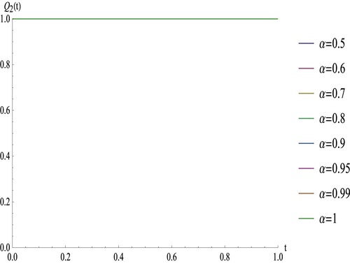The approximate solution for different values of α and m=50 are given in Figures 1 and 2. We should note that from Figure 2, since the solution $Q_2$ is constant and equal to one, we observe that the approximate solutions of $Q_2$ for different values of α form the same horizontal line, $Q_2\left(t\right)=1$.

Figure 1. Approximate solutions of $Q_1$ for different values of α of Example 6.1.

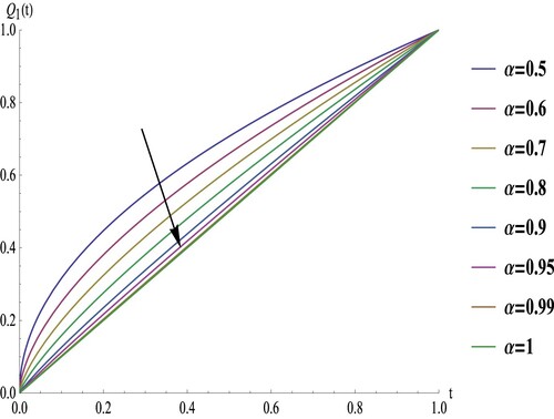
Figure 2. Approximate solutions of $Q_2$ for different values of α of Example 6.1.

Simple calculations imply that (70) $\begin{array}{rl}\underset{m\to \mathrm{\infty }}{lim}\underset{\alpha \to 1}{lim}{Q}_{1,m}\left(t\right)& =\underset{m\to \mathrm{\infty }}{lim}\underset{\alpha \to 1}{lim}\sum _{j=0}^{m-1}{q}_{1,j}{\text{β}}_j\left(t\right)=\underset{m\to \mathrm{\infty }}{lim}\sum _{j=0}^{m-1}\frac{(j+1{)}^2-j^2}{2m}{\text{β}}_j\left(t\right)=x,\end{array}$(70) (71) $\begin{array}{rl}\underset{m\to \mathrm{\infty }}{lim}\underset{\alpha \to 1}{lim}{Q}_{2,m}\left(t\right)& =\underset{m\to \mathrm{\infty }}{lim}\underset{\alpha \to 1}{lim}\sum _{j=0}^{m-1}{q}_{2,j}{\text{β}}_j\left(t\right)=\sum _{j=0}^{\mathrm{\infty }}{\text{β}}_j\left(t\right)=1,\end{array}$(71) which converges to the exact solution of the model given in [16] and [37] for $\alpha =1$. In the next two examples, we use the same procedure but we report the results only without the details since we explain them in this example.

Example 6.2

[19,36,38,39] Consider the following system $\begin{array}{rl}& D^{\alpha }{Q}_1\left(t\right)=Q_1\left(t\right)(1-\frac{1}{3}{Q}_2(t)-{\int }_{t-\frac{1}{2}}^t{Q}_2\left(s\right)\mathrm{d}s)+f_1\left(t\right),\\ & D^{\alpha }{Q}_2\left(t\right)=Q_2\left(t\right)(-2+Q_1(t)+{\int }_{t-\frac{1}{2}}^t(t-s-1)Q_1\left(s\right)\mathrm{d}s)+f\left(t\right),\end{array}$with $Q_1\left(0\right)=1,Q_2\left(0\right)=0.$and $\begin{array}{rl}{f}_1\left(t\right)& =-3\mathrm{\Gamma }(\alpha +1)\\ & -(1-3t^{\alpha })(1-\frac{t^{2\alpha }}{3}+\frac{t^{\alpha }}{3}+\frac{(t-\frac{1}{2}{)}^{2\alpha +1}-t^{2\alpha +1}}{2\alpha +1}+\frac{t^{\alpha +1}-(t-\frac{1}{2}{)}^{\alpha +1}}{\alpha +1}),\\ f_2\left(t\right)& =\frac{\mathrm{\Gamma }(2\alpha +1)}{\mathrm{\Gamma }(\alpha +1)}{t}^{\alpha }-\mathrm{\Gamma }(\alpha +1)\\ & -(t^{2\alpha +2}-t^{\alpha })(\frac{3t^{\alpha +2}-3(t-\frac{1}{2}{)}^{\alpha +2}}{\alpha +2}+\frac{(3-3t)(t^{\alpha +1}-(t-\frac{1}{2}{)}^{\alpha +1}}{\alpha +1}-3t^{\alpha }-\frac{11}{8}).\end{array}$

Then, ${\eta }_1=1,{\eta }_2=2,{\omega }_1=\frac{1}{3},{\omega }_2=1,\mathrm{\Delta }=\frac{1}{2}$. Moreover, the Kernels $K_1\left(t\right)=1,K_2\left(t\right)=t-1$. When $\alpha =1$, the exact solution is $Q_1\left(t\right)=-3t+1$ and $Q_2\left(t\right)=t^2-t$. Following the procedure described in Example 6.1, we get (72) $\begin{array}{rl}{q}_{1,j}& =\frac{\alpha +3j{\left(\frac{j-1}{m}\right)}^{\alpha }-3{\left(\frac{j-1}{m}\right)}^{\alpha }-3j{\left(\frac{j}{m}\right)}^{\alpha }+1}{\alpha +1},\end{array}$(72) (73) $\begin{array}{rl}{q}_{2,j}& =\frac{(2\alpha +1)(-j){\left(\frac{j}{m}\right)}^{\alpha }+(\alpha +1)j{\left(\frac{j}{m}\right)}^{2\alpha }+m{\left(\frac{j-1}{m}\right)}^{\alpha +1}(2\alpha -(\alpha +1){\left(\frac{j-1}{m}\right)}^{\alpha }+1)}{(\alpha +1)(2\alpha +1)},\end{array}$(73)

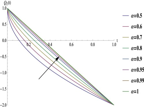
for $j=0,1,\dots ,m-1$. The approximate solution for different values of α and m=50 are given in Figures 3 and 4. We will compare our results produced by the operational matrix method (OMM) with Adomian decomposition method (ADM) [36], variational iteration method (VIM) [19], Taylor collocation method (TCM) [38], and Legendre method (LM) [39]. The absolute errors $e_1\left(t_i\right)=\mid Q_1\left(t_i\right)-Q_{1}app\left(t_i\right)\mid ,e_2\left(t_i\right)=\mid Q_2\left(t_i\right)-Q_{2}app\left(t_i\right)\mid .$are reported in Tables 1 and 2. In our approach we use m=25.

Figure 3. Approximate solutions of $Q_1$ for different values of α of Example 6.2.

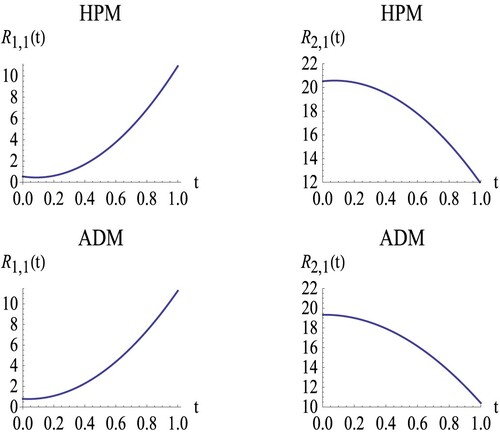
Example 6.3

[40,41] Consider the following system $\begin{array}{rl}& D^{\alpha }{Q}_1\left(t\right)=Q_1\left(t\right)(0.02-0.01Q_2(t)-{\int }_{t-0.1}^t{e}^{-(t-s)}{Q}_2\left(s\right)\mathrm{d}s),\\ & D^{\alpha }{Q}_2\left(t\right)=Q_2\left(t\right)(-0.01+0.01Q_1(t)+{\int }_{t-0.1}^t{e}^{-(t-s)}{Q}_1\left(s\right)\mathrm{d}s),\end{array}$with $Q_1\left(0\right)=10,Q_2\left(0\right)=10.$Then, ${\eta }_1=0.02,{\eta }_2=0.01,{\omega }_1={\omega }_2=0.01,\mathrm{\Delta }=0.1$. Moreover, the Kernels $K_1\left(t\right)=k_2\left(t\right)=e^{-t}$. When $\alpha =1$, the approximate solution using HPM [40] is $Q_1\left(t\right)=0.1557t^2-10.6162t+10$ and $Q_2\left(t\right)=10+10.4163t+\frac{t^2}{2000}$ while the approximate solutions using the ADM [41] is $Q_1\left(t\right)=10-10.3162t+0.02t^2$ and $Q_2\left(t\right)=10+11.6162t+\frac{t^2}{2000}$. Since the exact solution of this system is unknown, we define another measure for the error which is the residual errors by $\begin{array}{rl}& R_{1,\alpha }\left(t\right)=\mid D^{\alpha }{Q}_1\left(t\right)-Q_1\left(t\right)(0.02-0.01Q_2(t)-{\int }_{t-0.1}^t{e}^{-(t-s)}{Q}_2\left(s\right)\mathrm{d}s)\mid ,\\ & R_{2,\alpha }\left(t\right)=\mid D^{\alpha }{Q}_2\left(t\right)-Q_2\left(t\right)(-0.01+0.01Q_1(t)+{\int }_{t-0.1}^t{e}^{-(t-s)}{Q}_1\left(s\right)\mathrm{d}s)\mid ,\end{array}$For the fractional case, we should note the operational matrix of $D^{\alpha }$ is ${\mathrm{\Omega }}_2^{-1}$. Thus, the residual error for the fractional case is (74) $\begin{array}{rl}& R_{1,\alpha }\left(t\right)=\mid (P_1{\mathrm{\Omega }}_2^{-1}-({\eta }_1{P}_1-{\omega }_1{P}_1\odot P_2-\frac{1}{h}{P}_1\odot P_2{\mathrm{\Pi }}_1+F_1))\text{β}\left(t\right)\mid ,\end{array}$(74) (75) $\begin{array}{rl}& R_{2,\alpha }\left(t\right)=\mid (P_2{\mathrm{\Omega }}_2^{-1}-(-{\eta }_2{P}_2+{\omega }_2{P}_1\odot P_2+\frac{1}{h}{P}_2\odot P_1{\mathrm{\Pi }}_2+F_2))\text{β}\left(t\right)\mid .\end{array}$(75) Following the procedure described in Example 6.1, the residual error for $\alpha =0.8$ and 1.0 are reported in Table 3 for m=50. Also, the residual errors for $\alpha =1$ using HPM and ADM are given in Figure 5.

Table 1. The absolute errors for $Q_1\left(t\right)$ when $\alpha =1$.

$t_i$	ADM	VIM	TCM	LM	OMM
0.1	$1.1\ast {10}^{-4}$	$3.2\ast {10}^{-4}$	$0.54\ast {10}^{-12}$	$2.0\ast {10}^{-13}$	$2.4\ast {10}^{-16}$
0.2	$1.8\ast {10}^{-4}$	$4.3\ast {10}^{-4}$	$0.10\ast {10}^{-11}$	$3.2\ast {10}^{-13}$	$2.2\ast {10}^{-16}$
0.3	$1.1\ast {10}^{-4}$	$4.7\ast {10}^{-4}$	$0.13\ast {10}^{-11}$	$3.6\ast {10}^{-13}$	$1.8\ast {10}^{-16}$
0.4	$3.1\ast {10}^{-4}$	$4.9\ast {10}^{-4}$	$0.15\ast {10}^{-11}$	$3.2\ast {10}^{-13}$	$1.9\ast {10}^{-16}$
0.5	$1.4\ast {10}^{-3}$	$4.7\ast {10}^{-4}$	$0.19\ast {10}^{-11}$	$2.1\ast {10}^{-13}$	$2.1\ast {10}^{-16}$
0.6	$1.4\ast {10}^{-3}$	$4.5\ast {10}^{-4}$	$0.23\ast {10}^{-11}$	$3.4\ast {10}^{-14}$	$2.4\ast {10}^{-16}$
0.7	$6.4\ast {10}^{-3}$	$4.4\ast {10}^{-4}$	$0.29\ast {10}^{-11}$	$2.0\ast {10}^{-13}$	$3.1\ast {10}^{-15}$
0.8	$1.1\ast {10}^{-2}$	$5.4\ast {10}^{-4}$	$0.36\ast {10}^{-11}$	$4.8\ast {10}^{-13}$	$2.7\ast {10}^{-15}$
0.9	$1.5\ast {10}^{-2}$	$9.1\ast {10}^{-4}$	$0.45\ast {10}^{-11}$	$8.1\ast {10}^{-13}$	$1.9\ast {10}^{-15}$
1.0	$2.0\ast {10}^{-2}$	$1.8\ast {10}^{-3}$	$0.83\ast {10}^{-11}$	$1.2\ast {10}^{-12}$	$2.1\ast {10}^{-15}$

Table 2. The absolute errors for $Q_2\left(t\right)$ when $\alpha =1$.

$t_i$	ADM	VIM	TCM	LM	OMM
0.1	$7.6\ast {10}^{-6}$	$3.3\ast {10}^{-5}$	$0.59\ast {10}^{-11}$	$4.5\ast {10}^{-14}$	$6.3\ast {10}^{-15}$
0.2	$1.5\ast {10}^{-8}$	$8.5\ast {10}^{-5}$	$0.38\ast {10}^{-11}$	$3.7\ast {10}^{-14}$	$6.1\ast {10}^{-15}$
0.3	$7.7\ast {10}^{-4}$	$1.3\ast {10}^{-4}$	$0.34\ast {10}^{-11}$	$1.1\ast {10}^{-14}$	$4.9\ast {10}^{-15}$
0.4	$2.8\ast {10}^{-3}$	$1.8\ast {10}^{-4}$	$0.26\ast {10}^{-11}$	$9.0\ast {10}^{-14}$	$3.8\ast {10}^{-15}$
0.5	$7.6\ast {10}^{-3}$	$2.2\ast {10}^{-4}$	$0.21\ast {10}^{-11}$	$1.9\ast {10}^{-13}$	$3.2\ast {10}^{-15}$
0.6	$1.8\ast {10}^{-2}$	$2.4\ast {10}^{-4}$	$0.17\ast {10}^{-11}$	$3.0\ast {10}^{-13}$	$3.8\ast {10}^{-15}$
0.7	$3.6\ast {10}^{-2}$	$1.6\ast {10}^{-4}$	$0.11\ast {10}^{-11}$	$4.1\ast {10}^{-13}$	$4.1\ast {10}^{-15}$
0.8	$6.7\ast {10}^{-2}$	$1.1\ast {10}^{-4}$	$0.15\ast {10}^{-11}$	$5.1\ast {10}^{-13}$	$6.2\ast {10}^{-14}$
0.9	$1.1\ast {10}^{-1}$	$7.3\ast {10}^{-4}$	$0.44\ast {10}^{-11}$	$5.8\ast {10}^{-13}$	$4.4\ast {10}^{-14}$
1.0	$1.8\ast {10}^{-1}$	$1.9\ast {10}^{-3}$	$0.25\ast {10}^{-9}$	$6.2\ast {10}^{-13}$	$2.8\ast {10}^{-14}$

Table 3. The residual errors for $\alpha =0.8,1$.

$t_i$	$R_{1,0.8}$	$R_{2,0.8}$	$R_{1,1}$	$R_{2,1}$
0.1	$0.5\ast {10}^{-4}$	$0.6\ast {10}^{-4}$	$0.5\ast {10}^{-4}$	$0.7\ast {10}^{-4}$
0.2	$0.4\ast {10}^{-4}$	$0.3\ast {10}^{-4}$	$0.4\ast {10}^{-4}$	$0.4\ast {10}^{-4}$
0.3	$0.6\ast {10}^{-4}$	$0.7\ast {10}^{-4}$	$0.7\ast {10}^{-4}$	$0.8\ast {10}^{-4}$
0.4	$1.0\ast {10}^{-4}$	$1.1\ast {10}^{-4}$	$1.1\ast {10}^{-4}$	$1.2\ast {10}^{-4}$
0.5	$1.7\ast {10}^{-4}$	$2.1\ast {10}^{-4}$	$1.7\ast {10}^{-4}$	$1.9\ast {10}^{-4}$
0.6	$2.6\ast {10}^{-4}$	$2.8\ast {10}^{-4}$	$2.5\ast {10}^{-4}$	$2.8\ast {10}^{-4}$
0.7	$3.7\ast {10}^{-4}$	$3.6\ast {10}^{-4}$	$2.9\ast {10}^{-4}$	$3.8\ast {10}^{-4}$
0.8	$5.2\ast {10}^{-4}$	$5.7\ast {10}^{-4}$	$4.1\ast {10}^{-4}$	$5.4\ast {10}^{-4}$
0.9	$6.9\ast {10}^{-4}$	$7.1\ast {10}^{-4}$	$5.3\ast {10}^{-4}$	$7.0\ast {10}^{-4}$
1.0	$8.8\ast {10}^{-4}$	$9.1\ast {10}^{-4}$	$7.9\ast {10}^{-4}$	$8.9\ast {10}^{-4}$

7. Discussion of the results

In this paper, we test the proposed method using three different applications and conduct comparisons with other researchers. In the first example, we study a system of integro-differential equations, which is an application related to biological species living together. We then compare our results with those obtained using the ADM [36]. In the second example, we explore another application from mathematical biology and compare our results with those from ADM [36], VIM [19], TCM [38], and LM [39]. Finally, we solve the third problem in the field of mathematical biology and compare our results with those from [40,41].

From these examples, we made the following observations:

• In Example 6.1, we observed that the solution of the fractional system (1(1) $\begin{array}{rl}{D}^{\alpha }{Q}_1\left(t\right)& =Q_1\left(t\right)({\eta }_1-{\omega }_1{Q}_2(t)-{\int }_{t-\mathrm{\Delta }}^t{K}_1(t-s)Q_2\left(s\right)\mathrm{d}s)+f_1\left(t\right),\end{array}$(1) )–(3(3) $Q_1\left(0\right)=a_1,Q_2\left(0\right)=a_2,$(3) ) converges to the exact solution when $\alpha =1$. Our findings are in line with those presented in [36]. Furthermore, based on Figures 1 and 2, it is evident that the profile of $Q_1\left(t\right)$ decreases as α increases within the interval $[0,1]$, while the profile of $Q_2\left(t\right)$ remains constant with increasing α.

• In Example 6.2, as depicted in Figures 3 and 4, it is apparent that the profile of $Q_1\left(t\right)$ increases as α rises within the interval $[0,1]$. However, the behaviour of $Q_2\left(t\right)$ differs between the intervals $[0,0.4]$ and $[0.4,1]$, where it increases initially and then decreases as α increases. When $\alpha =1$, we compared our results with ADM [36], VIM [19], TCM [38], and LM [39]. We found that OMM yields superior results, as shown in Tables 1 and 2. We employed the absolute error as a measure of accuracy for the proposed method and for comparisons with other approaches.

• In Example 6.3, where the exact solution is unknown, we defined the residual error. Our results, reported in Table 3, showed that the residual error is within ${10}^{-4}$ for $\alpha =0.8$ and 1.0. We compared our results with [40,41], as shown in Figure 5, and noted that the residual error exceeds 10 at some points, with the minimum value for $R_{1,1}\left(t\right)$ being about 0.5, while the minimum value for $R_{2,1}\left(t\right)$ is approximately 10. This demonstrates that our results, using OMM, are superior as the residual error remains within ${10}^{-4}$.

Figure 4. Approximate solutions of $Q_2$ for different values of α of Example 6.2.

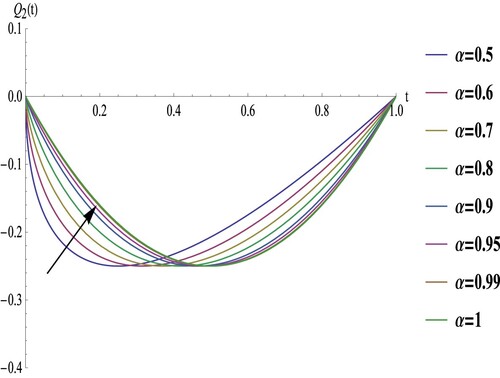
Figure 5. Residual errors for $\alpha =1$ using HPM and ADM of Example 6.3.

8. Conclusions

In this paper, we have explored the solution of a nonlinear system of fractional integro-differential equations in the Caputo sense, a system with significant relevance in various scientific applications. Our approach to solving this system involved the utilization of the operational matrix method, where we derived the operational matrices in Section 3 and detailed the solution method in Section 4.

Throughout our study, we established several crucial theoretical results, including the proof of existence and uniqueness of solutions for system (1(1) $\begin{array}{rl}{D}^{\alpha }{Q}_1\left(t\right)& =Q_1\left(t\right)({\eta }_1-{\omega }_1{Q}_2(t)-{\int }_{t-\mathrm{\Delta }}^t{K}_1(t-s)Q_2\left(s\right)\mathrm{d}s)+f_1\left(t\right),\end{array}$(1) )–(3(3) $Q_1\left(0\right)=a_1,Q_2\left(0\right)=a_2,$(3) ). We also delved into the topics of Ulam–Hyers stability and generalized Ulam–Hyers stability. Furthermore, we provided insights into three illustrative examples and compared our results with various methods, including ADM [36,41], VIM [19], TCM [38], and LM [39].

From the analysis of these examples, it becomes evident that the proposed method is practical, offers increased accuracy compared to alternative methods, and significantly reduces computational time and costs. Additionally, we considered these examples as applications from mathematical biology, specifically addressing biological species living together.

Author contributions

The authors confirm contribution to the paper as follows: All authors have equal contribution. All authors reviewed the results and approved the final version of the manuscript.

Disclosure statement

No potential conflict of interest was reported by the author(s).

Additional information

Funding

The authors would like to thank the Deanship of Scientific Research at Umm Al-Qura University for supporting this work [grant code: 23UQU4310382DSR03].

References

- Baleanu D, Jaiami A, Sajjadi S, et al. A new fractional model and optimal control of a tumor-immune surveillance with non-singular derivative operator. Chaos. 2019;29(8):083–127. doi: 10.1063/1.5096159
- Caputo M, Fabrizio M. A new definition of fractional derivative without singular kernel. Prog Fract Differ Appl. 2015;1(2):73–85.
- Kilbas AA, Srivastava HM, Trujillo JJ. Theory and applications of fractional differential equations. North-Holland math. studies. Amsterdam: Elsevier; 2006.
- Arora S, Mathur T, Agarwal S, et al. Applications of fractional calculus in computer vision: a survey. Neurocomputing. 2022;489:407–428. doi: 10.1016/j.neucom.2021.10.122
- Rahman M, Arfan M, Deebani W, et al. Analysis of time-fractional Kawahara equation under Mittag–Leffler power law. Fractals. 2022;30(01):Article ID 2240021. doi: 10.1142/S0218348X22400217
- Anjam YN, Shafqat R, Sarris IE, et al. A fractional order investigation of smoking model using caputo-Fabrizio differential operator. Fractal Fract . 2022;6:623. doi: 10.3390/fractalfract6110623
- Adnan Ali A, Shah Z, Kumam P. Investigation of a time-fractional COVID-19 mathematical model with singular kernel. Adv Cont Discr Mod. 2022;2022:34. doi: 10.1186/s13662-022-03701-z
- Xu C, Rahman MU, Fatima B, et al. Theoretical and numerical investigation of complexities in fractional-order chaotic system having torus attractors. Fractals. 2022;30:Article ID 2250164. doi: 10.1142/S0218348X2250164X
- Rahman M, Althobaiti A, Riaz MB, et al. A theoretical and numerical study on fractional order biological models with caputo fabrizio derivative. Fractal Fract. 2022;6:446. doi: 10.3390/fractalfract6080446
- Haidong Q, Al Hazmi SE, Yassen MF, et al. Analysis of non-equilibrium 4D dynamical system with fractal fractional Mittag–Leffer kernel. Eng Sci Technol. 2023;37:Article ID 101319. doi: 10.1016/j.jestch.2022.101319
- Wang M, Karaca Y, Zhou M. A theoretical view of existence results by using fixed point theory for quasi-variational inequalities. Appl Math Sci Eng. 2023;31:1. doi: 10.1080/27690911.2023.2167990
- Amin R, Ahmad H, Shah K, et al. Theoretical and computational analysis of nonlinear fractional integro-differential equations via collocation method. Chaos Solitons Fractals. 2021;151:Article ID 111252. doi: 10.1016/j.chaos.2021.111252
- Biazar J, Sadri K. Solution of weakly singular fractional integro-differential equations by using a new operational approach. J Comput Appl Math. 2019;352:453–477. doi: 10.1016/j.cam.2018.12.008
- Sahu P, Saha Ray S. Legendre spectral collocation method for the solution of the model describing biological species living together. J Comput Appl Math. 2016;296:47–55. doi: 10.1016/j.cam.2015.09.011
- Jerri AJ. Introduction to integral equations and applications. New York: John Wiley and Sons Inc; 1999.
- Bourazza S, Altoum Sami H, Ayed H, et al. Discharging process within a storage container considering numerical method. J Energy Storage. 2023;66:Article ID 107490. doi: 10.1016/j.est.2023.107490
- Kilbas AA, Srivastava HM, Trujillo JJ. Theory and applications of fractional differential equations. Amsterdam: Elsevier; 2006.
- Roul P, Meyer P. Numerical solutions of systems of nonlinear-differential equations by homotopy-perturbation method. Appl Math Model. 2011;35:4234–4242. doi: 10.1016/j.apm.2011.02.043
- Shakeri F, Dehghan M. Solution of a model describing biological species living together using the variational iteration method. Math Comput Model. 2008;48:685–699. doi: 10.1016/j.mcm.2007.11.012
- Youbi F, Momani S, Hasan S, et al. Effective numerical technique for nonlinear Caputo-Fabrizio systems of fractional volterra integro-differential equations in Hilbert space. Alexandria Eng J. 61(3):1778–1786. doi: 10.1016/j.aej.2021.06.086
- Akbar M, Nawaz R, Ahsan S, et al. New approach to approximate the solution for the system of fractional order volterra integro-differential equations. Results Phys. 2020;19:Article ID 103453. doi: 10.1016/j.rinp.2020.103453
- Jangveladze T, Kiguradze Z, Neta B. Finite difference approximation of a nonlinear integro-differential system. Appl Math Comput. 2009;215(2):615–628. doi: 10.1016/j.amc.2009.05.061.
- Wei L, Agarwal RP, Wong PJ. Discussion on the existence and uniqueness of solution to nonlinear integro-differential systems. Comput Math Appl. 2015;69(5):374–389. doi: 10.1016/j.camwa.2014.12.007.
- Syam SM, Siri Z, Altoum SH, et al. An efficient numerical approach for solving systems of fractional problems and their applications in science. Mathematics. 2023;11(14):3132. doi: 10.3390/math11143132
- Syam SM, Yildirim K. A new method for solving sequential fractional wave equations. J. Math.. 2023;2023:Article ID 5888010–16. doi: 10.1155/2023/5888010
- Hatamzadeh-Varmazyar S, Masouri Z, Babolian E. Numerical method for solving arbitrary linear differential equations using a set of orthogonal basis functions and operational matrix. Appl Math Model. 2016;40(1):233–253. doi: 10.1016/j.apm.2015.04.048.
- Najafalizadeh S, Ezzati R. A block pulse operational matrix method for solving two-dimensional nonlinear integro-differential equations of fractional order. J Comput Appl Math. 2017;326:159–170. doi: 10.1016/j.cam.2017.05.039
- Zamanpour I, Ezzati R. Operational matrix method for solving fractional weakly singular 2D partial volterra integral equations. J Comput Appl Math. 2023;419:Article ID 114704. doi: 10.1016/j.cam.2022.114704
- Syam MI, Sharadga M, Hashim I. A numerical method for solving fractional delay differential equations based on the operational matrix method. Chaos Solitons Fractals. 2021;147:Article ID 110977. doi: 10.1016/j.chaos.2021.110977
- Altoum Sami H, Syam Muhammed I, Syam Sondos M, et al. Effcacy of magnetic force on nanofuid laminar transportation and convective fow. J Magn Magn Mater. 2023;581:Article ID 170964. doi: 10.1016/j.jmmm.2023.170964
- Syam SM, Siri Z, Kasmani R M. “Operational matrix method for solving fractional system of riccati equations,” 2023 International Conference on Fractional Differentiation and Its Applications (ICFDA); 2023. p. 1–6; Ajman, United Arab Emirates. doi: 10.1109/ICFDA58234.2023.10153350
- Syam SM, Zailan S, Altoum SH, et al. Analytical and numerical methods for solving second-Order two-Dimensional symmetric sequential fractional integro-differential equations. Symmetry. 2023;15:1263. doi: 10.3390/sym15061263
- Samko SG, Kilbas AA, Marichev OI. Fractional integrals and derivatives: theory and applications. Yverdon: Gordon and Breach; 1993.
- Podlubny I. Fractional differential equations. San Diego: Academic Press; 1999.
- Khan A, Syam MI, Zada A, et al. Stability analysis of nonlinear fractional differential equations with Caputo and Riemann-Liouville derivatives. Eur Phys J Plus. 2018;133:264. doi: 10.1140/epjp/i2018-12119-6
- Babolian E, Biazar J. Solving the problem of biological species living together by adomian decomposition method. Appl Malt Comput. 2002;129:339–343.
- Hassan I, Collins A, Obiajulu O. The revised new iterative method for solving the model describing biological species living together. Amer J Comput Appl Math. 2016;6(3):136–143. doi: 10.5923/j.ajcam.20160603.03.
- Gokmen E, Sezer M. Approximate solution of a model describing biological species living together by Taylor collocation method. New Trends Math Sci. 2005;3(2):147–158.
- Yousefi SA. Numerical solution of a model describing biological species living together by using Legendre multiwalet method. Int J Nonlinear Sci. 2011;11(1):109–113.
- Biazar J, Ayati Z, Partovi M. Homotopy perturbation method for biological species living together. Int J Appl Math Res. 2013;2(1):44–48.
- Babolian E, Biazar J. Solving the problem of biological species living together by adomian decomposition method. Appl Math Comput. 2002;129:339–343. doi: 10.1016/S0096-3003(01)00043-1