Analysis and estimation of the COVID-19 pandemic by modified homotopy perturbation method

Abstract

The Bernoulli equation is useful to assess the motility and recovery rate with respect to time in order to measure the COVID-19 outbreak. The homotopy perturbation method was applied in the current article to compute the Bernoulli equation. For the existence and uniqueness of solutions, we also used the Caputo–Fabrizio Integral and differential operators. Additionally, we conducted a corresponding investigation for derivatives of integer and fractional orders on the estimated motility and recovery rate.

Keywords:

• SARS-CoV-2
• homotopy decomposition method (HDM)
• ODE
• COVID-19
• mathematical modelling

Mathematics Subject Classifications:

• 92-10
• 49M27
• 34A12

1. Introduction

Globally, the coronavirus COVID-19 has spread. There are numerous mathematical models available for analysing the patterns and rough solutions to this epidemic. This virus originated in Wuhan, China, as is well known. The worldometer website, which is accessible online, states that the number of infected people in China is at an all-time high in the month of May. There are over 4 million instances of the coronavirus in the final week of May. Cherniha [1] proposed a Mathematical Model for the Corona.

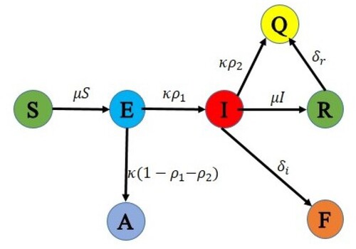
The first model of this pandemic is known as the SIR (Susceptible-Infectious-Recovered) model which includes three ODE's is the most common model defined by Cooper [2] and the dynamic chart of the behaviour is given in Figure 1. After this model [3] gives the SEIR model for the outbreak of COVID-19 with the appropriate parameters as shown in Figure 2. In the continuation of getting the approximate solutions of the COVID-19 model, Pang [4] studied SEIQRD Model (Susceptible-Exposed-Infectious-Quarantine-Recovered-Death) with the more generalization of types of infected people as given in Figure 3. Similarly, Cherniha [1] proposed the SEAIRQF (Susceptible-Exposed-Asymptomatic-Infectious-Recovered-Quarantined-Fatility class) Model using the asymptomatic exposed behaviour given in Figure 4. Anirudh [5] described the outcome and the challenges of these models mentioned above using the study of corona behaviour.

Figure 1. The progression of the dynamic of SIR model.

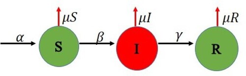
Figure 2. The progression of the dynamic of SEIR model.

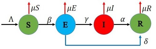
Figure 3. The progression of the dynamic of SEIQDR model.

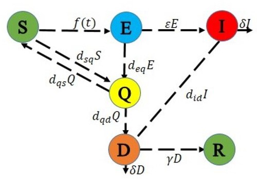
Figure 4. The progression of the dynamic of SEAIQRF model.

The flow chart of these mathematical models is given as:

In the year of 2020, Nisar [6,7] studied a Bats-hosts-reservoir People transmission fractional order COVID-19 model which was controlled and measured by the government.

Also, Thabet [8] proposed a mathematical model of COVID-19 under nonsingular derivative of fractional order.

For the prediction of this pandemic in different states of India, Jaspreet [9] also gave a preprint-based mathematical model of prediction of COVID-19. In May 2020, Ning [10] developed reliable epidemiological models to forecast the evolution of the virus and estimate the effectiveness of various intervention measures and their impacts on the economy. This was the first model based on the impact on economic conditions.

The numerical solution using Runge Kutta fourth-order method for this epidemic [11] gave a mathematical model with a nonstandard finite difference (NSFD) scheme and the wavelet based `numerical scheme for fractional order SEIR epidemic is discussed by Kumar et al. [12].

Ali et al. [13] also introduced a mathematical model for the study of the HIV-1 virus.

In the same manner, Izhan [14] used a hybrid model and a hybrid model and Ghosh et al. [15] studied the fractional model for population dynamics.

In the fractional order analysis with the comparison of this work in COVID, more study was also done [16–18].

The relationship of the mentioned model with the literature and comparison results are also reflected in the papers, in which Yavuz et al. studied about diabetes and hereditary and COVID-10 treatment rate [18–20].

Also in the cure of cancer, Altun [21] analysed Quantitative and numerical simulation. In the field of plant-pathogen herbivore interaction, Rahman [22] did a piecewise fractional analysis of the migration effect. In a similar manner, Joshi [17] analysed the stability of a non-singular fractional-order COVID-19 model with nonlinear incidence and treatment rate and Laxmi [16] studied on the vaccinational model for incorporating environmental transmission.

For the loss of immunity and quarantined class, Arif [23] gave models and numerical simulations and non-linear Burgers' equations via a semi-analytical technique [24].

A Modified Homotopy Perturbation Transform Method (Fractional-Order Newell-Whitehead-Segel Equation) is also analysed by N. Iqbal, A.M. Albalahi, M.S. Abdo and W. Mohammed [25].

In this direction the studies are also relatable to the comparison of this method given by Zeb et al. [26], Evirgin et al. [27], Ozkose [28], Jha [29], Naik [18,30]

In this paper, we applied the first nontrivial biological model (Logistic model) given by Verhulst [31] in the proposition of COVID-19 mathematical model by two smooth function $\zeta \left(\tau \right)$ (total arised cases) and $\phi \left(\tau \right)$ (total deaths) so that the study of behaviour of these graphs with the comparison of fractional order, Integer order and exact solution could be analysed.

The flow chart of this model is given in Figure 5.

Figure 5. Flow chart of total cases $\zeta \left(\tau \right)$ including total recovered $\sigma \left(\tau \right)$and deaths $\phi \left(\tau \right)$.

2. Methodology

2.1. Homotopy decomposition method and modified homotopy perturbation method

It is the most practical technique to utilize recently in fractional calculus. This method of fractional derivatives provides numerous general instances of the fractional derivative model. Its use in the area of fractional calculus in applied mathematics is therefore more pertinent.

Atangana and Botha (2012) were the first to develop the Homotopy Decomposition Method (HDM) to solve partial differential equations, which are frequently encountered in problems involving heat diffusion, time fraction, groundwater flow, etc.

Since the modified Homotopy perturbation method is used in this paper along with Adomian polynomials, it is technically a modified Homotopy perturbation approach.

Baleanu et al. [32] also presented a fractional order model.

2.2. The mathematical model

In 1838, Verhulst [31] developed the first nontrivial biological model. This model is also known as the Logistic Model. The ODE of this model is given by (1) $\frac{\mathrm{d}\mathrm{\Psi }}{\mathrm{d}\tau }=\mathrm{\Psi }(1-\mathrm{\Psi }),\mathrm{\Psi }\left(0\right)={\mathrm{\Psi }}_0.$(1) It is the classical example of Mathematical Biology. The exact solution of this model is (2) $\mathrm{\Psi }\left(\tau \right)=\frac{{\mathrm{\Psi }}_0{e}^{\tau }}{1+{\mathrm{\Psi }}_0(e^{\tau }-1)}.$(2) Its curve is sigmoid (logistic) and useful for fractional value ${\mathrm{\Psi }}_0<1/2$. In this paper, we used HDM to find the approximate solution for the total people and death people and compare to integer and fractional order solution with the general function $\zeta \left(\tau \right)$ that denotes the number of the Corona cases identifying to day τ (for some integer). The initial cases at $\tau =0$ is $\zeta \left(0\right)={\zeta }_0$. Now let the general equation of this model be (3) $\frac{\mathrm{d}\zeta }{\mathrm{d}\tau }=\zeta (a-b{\zeta }^{\gamma }),\zeta \left(0\right)={\zeta }_0>0.$(3) a and b are here positive constants and τ is the exponent which confirms the number of Corona cases that bounds in time τ.

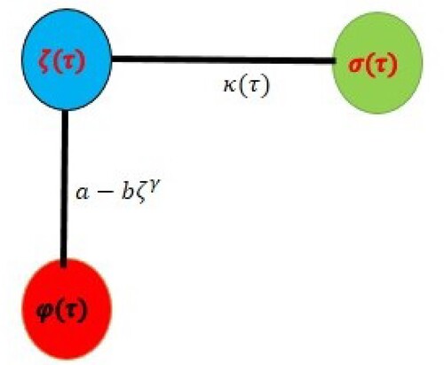
Ayala, Gilpin and Ehrenfeld in Ref. [33] introduced nonlinearity of (3(3) $\frac{\mathrm{d}\zeta }{\mathrm{d}\tau }=\zeta (a-b{\zeta }^{\gamma }),\zeta \left(0\right)={\zeta }_0>0.$(3) ) for describing the competition between species, while the logistic equation here shows some common assumptions by Brauer [34]. There are two possibilities for the infected person during the epidemic first one is φ which shows the population of dead persons and the other one is σ which represents the population of recovered persons from the corona. (4) $\zeta =\phi +\sigma .$(4) Now the ‘ which is directly proportional to total number ζ is (5) $\frac{\mathrm{d}\phi }{\mathrm{d}\tau }=k\left(\tau \right)\zeta ,\phi \left(0\right)={\phi }_0>0.$(5) Where $k\left(\tau \right)$ is the effectiveness coefficient of the system of health care in the process of epidemic and related to the expression $k\left(\tau \right)=k_0\mathrm{e}\mathrm{x}\mathrm{p}(-s\tau ),s>0.$All the parameters and defined functions are listed in Table 1:

Table 1. Table 1.

Notation	Meaning of parameters
$\zeta \left(\tau \right)$	At the time τ
The coronavirus cases
$\phi \left(\tau \right)$	At the time τ the dead people
$\sigma \left(\tau \right)$	Recovered people at the time τ
a	Modulus of spreading virus
b	Modulus of the government rules
γ	Bounding parameter in time τ
$k\left(\tau \right)$	Modulus of health care

The model (3(3) $\frac{\mathrm{d}\zeta }{\mathrm{d}\tau }=\zeta (a-b{\zeta }^{\gamma }),\zeta \left(0\right)={\zeta }_0>0.$(3) )–(5(5) $\frac{\mathrm{d}\phi }{\mathrm{d}\tau }=k\left(\tau \right)\zeta ,\phi \left(0\right)={\phi }_0>0.$(5) ) is used under essential simplifications of the epidemic process where it is assumed that $\zeta >>\phi$ Also, it is known that this pandemic is so severe that the rate of mortality is quite greater, which means the prediction $\zeta >>\phi$ is wrong and hence in this epidemic not useful. For example, $v\cong 0.14u$ in Italy [35]. In that type of case, the above-mentioned mathematical model (3(3) $\frac{\mathrm{d}\zeta }{\mathrm{d}\tau }=\zeta (a-b{\zeta }^{\gamma }),\zeta \left(0\right)={\zeta }_0>0.$(3) )–(5(5) $\frac{\mathrm{d}\phi }{\mathrm{d}\tau }=k\left(\tau \right)\zeta ,\phi \left(0\right)={\phi }_0>0.$(5) ) would be more specified using the difference factor ($\zeta -\varphi$) [since $\zeta >>\phi$] instead of a single function as follows (6) $\begin{array}{rl}& \frac{\mathrm{d}\zeta }{\mathrm{d}\tau }=(\zeta -\phi )(a-b(\zeta -\phi {)}^{\gamma }),\zeta (0)={\zeta }_0,\end{array}$(6) (7) $\begin{array}{rl}& \frac{\mathrm{d}\phi }{\mathrm{d}\tau }=k\left(\tau \right)(\zeta -\phi ),\phi \left(0\right)={\phi }_0.\end{array}$(7) Now from (4(4) $\zeta =\phi +\sigma .$(4) ) it is clear that $\sigma =(\zeta -\phi )$, so (8) $\frac{d\sigma }{\mathrm{d}\tau }=\frac{\mathrm{d}\zeta }{\mathrm{d}\tau }-\frac{\mathrm{d}\phi }{\mathrm{d}\tau },$(8) using (6(6) $\begin{array}{rl}& \frac{\mathrm{d}\zeta }{\mathrm{d}\tau }=(\zeta -\phi )(a-b(\zeta -\phi {)}^{\gamma }),\zeta (0)={\zeta }_0,\end{array}$(6) ) and (7(7) $\begin{array}{rl}& \frac{\mathrm{d}\phi }{\mathrm{d}\tau }=k\left(\tau \right)(\zeta -\phi ),\phi \left(0\right)={\phi }_0.\end{array}$(7) ) in (8(8) $\frac{d\sigma }{\mathrm{d}\tau }=\frac{\mathrm{d}\zeta }{\mathrm{d}\tau }-\frac{\mathrm{d}\phi }{\mathrm{d}\tau },$(8) ), we get (9) $\frac{\mathrm{d}\zeta }{\mathrm{d}\tau }=\sigma (a-b{\sigma }^{\gamma }).\zeta \left(0\right)={\zeta }_0,$(9) And (10) $\frac{\mathrm{d}\phi }{\mathrm{d}\tau }=k\left(\tau \right)\sigma ,\phi \left(0\right)={\phi }_0.$(10) This equation (9(9) $\frac{\mathrm{d}\zeta }{\mathrm{d}\tau }=\sigma (a-b{\sigma }^{\gamma }).\zeta \left(0\right)={\zeta }_0,$(9) ) is called Bernoulli equation.

These Equations (9(9) $\frac{\mathrm{d}\zeta }{\mathrm{d}\tau }=\sigma (a-b{\sigma }^{\gamma }).\zeta \left(0\right)={\zeta }_0,$(9) ) and (10(10) $\frac{\mathrm{d}\phi }{\mathrm{d}\tau }=k\left(\tau \right)\sigma ,\phi \left(0\right)={\phi }_0.$(10) ) are time evolution equations of total cases and dead people. Now our aim is to compare these equations solutions by plotting the graphs between integer and fractional order.

For this first of all applying fractional order derivative [36] on (9(9) $\frac{\mathrm{d}\zeta }{\mathrm{d}\tau }=\sigma (a-b{\sigma }^{\gamma }).\zeta \left(0\right)={\zeta }_0,$(9) ) and (10(10) $\frac{\mathrm{d}\phi }{\mathrm{d}\tau }=k\left(\tau \right)\sigma ,\phi \left(0\right)={\phi }_0.$(10) ) (11) $\begin{array}{rl}& D_{\tau }^{\alpha }\left[\zeta \right(\tau \left)\right]=\sigma \left(\tau \right)[a-b{\sigma \left(\tau \right)}^{\gamma }],\end{array}$(11) (12) $\begin{array}{rl}& D_{\tau }^{\text{β}}\left[\phi \right(\tau \left)\right]=k\left(\tau \right)\sigma \left(\tau \right).\end{array}$(12) And the solutions are given by (13) $\begin{array}{rl}& \zeta \left(\tau \right)=\zeta \left(0\right)+\frac{1}{\mathrm{\Gamma }\left(\alpha \right)}{\int }_0^{\tau }(\tau -\theta {)}^{\alpha -1}[\sigma \left(\theta \right)[a-b{\sigma \left(\theta \right)}^{\gamma }]]\mathrm{d}\theta ,\end{array}$(13) (14) $\begin{array}{rl}& \phi \left(\tau \right)=\phi \left(0\right)+\frac{1}{\mathrm{\Gamma }\left(\text{β}\right)}{\int }_0^{\tau }(\tau -\theta {)}^{\alpha -1}[k\left(\theta \right)\sigma \left(\theta \right)]\mathrm{d}\theta .\end{array}$(14) Here the sets of kernels are $k_1(\tau ,\zeta )=\sigma \left(\tau \right)[a-b{\sigma \left(\tau \right)}^{\gamma }],$and $k_2(\tau ,\phi )=k\left(\tau \right)\sigma \left(\tau \right).$

2.3. Existence and uniqueness of model solution

The Lipschitz conditions give the existence and uniqueness condition for mathematical models, which are studied by Moore et al. [37] for HIV/AIDS, which is given with a treatment compartment.

In this section, we studied the existence and uniqueness condition by applying Caputo–Fabrizio fractional operators in (11(11) $\begin{array}{rl}& D_{\tau }^{\alpha }\left[\zeta \right(\tau \left)\right]=\sigma \left(\tau \right)[a-b{\sigma \left(\tau \right)}^{\gamma }],\end{array}$(11) ) and (12(12) $\begin{array}{rl}& D_{\tau }^{\text{β}}\left[\phi \right(\tau \left)\right]=k\left(\tau \right)\sigma \left(\tau \right).\end{array}$(12) ) on both sides, we get (15) $\begin{array}{rl}& \zeta \left(\tau \right)-\zeta \left(0\right)={}^{CF}{I}_t^{{\rho }_1}\left[\sigma \right(\tau \left)a-b\sigma (\tau {)}^{\gamma }\right],\end{array}$(15) (16) $\begin{array}{rl}& \phi \left(\tau \right)-\phi \left(0\right)={}^{CF}{I}_t^{{\rho }_2}\left[\kappa \right(\tau \left)\sigma \right(\tau \left)\right].\end{array}$(16) Where ${}^{CF}{I}_t^{\rho }$ is defined as the Caputo-fractional operator [38].

Then for simplicity, we define two kernels as follows: $k_1(\tau ,\zeta )=\sigma \left(\tau \right)[a-b{\sigma \left(\tau \right)}^{\gamma }],$and $k_2(\tau ,\phi )=k\left(\tau \right)\sigma \left(\tau \right).$For proving the theorems, we will suppose that ζ and φ are nonnegative bounded functions, that means $\Vert \zeta \left(\tau \right)\Vert \le {\theta }_1$, $\Vert \phi \left(\tau \right)\Vert \le {\theta }_2$. Where ${\theta }_1$ and ${\theta }_2$ are positive constants. Now represent (17) ${\mathrm{\Gamma }}_1=a-b\sigma (\tau {)}^{\gamma },{\mathrm{\Gamma }}_2=\kappa (\tau ).$(17) Applying the definition of the Caputo-Fabrizio fractional integral in (11(11) $\begin{array}{rl}& D_{\tau }^{\alpha }\left[\zeta \right(\tau \left)\right]=\sigma \left(\tau \right)[a-b{\sigma \left(\tau \right)}^{\gamma }],\end{array}$(11) ) and (12(12) $\begin{array}{rl}& D_{\tau }^{\text{β}}\left[\phi \right(\tau \left)\right]=k\left(\tau \right)\sigma \left(\tau \right).\end{array}$(12) ), we get (18) $\begin{array}{r}\zeta \left(\tau \right)-\zeta \left(0\right)=\mathrm{\Omega }\left({\rho }_1\right)k_1(\tau ,\zeta )+\omega \left({\rho }_1\right){\int }_0^{\tau }{k}_1(y,\zeta )\mathrm{d}y,\\ \phi \left(\tau \right)-\phi \left(0\right)=\mathrm{\Omega }\left({\rho }_2\right)k_2(\tau ,\phi )+\omega \left({\rho }_2\right){\int }_0^{\tau }{k}_2(y,\phi )\mathrm{d}y.\end{array}$(18) where the integral function is defined as: $\mathrm{\Omega }\left(\rho \right)=\frac{2(1-\rho )}{(2-\rho )M\left(\rho \right)},$and (19) $\omega \left(\rho \right)=\frac{2\rho }{(2-\rho )M\left(\rho \right)}.$(19) in which ρ is known as the order parameter.

2.4. Theorem 1

If the following inequality holds (20) $0\le M=max\left({\mathrm{\Gamma }}_1,{\mathrm{\Gamma }}_2\right)<1.$(20) Then the kernels $k_1$, and $k_2$ satisfy Lipschitz conditions and are contraction mappings.

Proof: We consider the kernels $k_1$. Let ζ and ${\zeta }_1$ are any two functions, then we have (21) $\Vert k_1(\tau ,\zeta )-k_1(\tau ,{\zeta }_1)\Vert =\Vert a\left[\sigma \right(\tau )-{\sigma }_1(\tau \left)\right]-b\left[\sigma \right(\tau {)}^{\gamma }-{\sigma }_1\left(\tau {)}^{\gamma }\right]\Vert .$(21) With the help of the norms of triangle inequality on the right side of the above equation, we get (22) $\begin{array}{rl}& \Vert k_1(\tau ,\zeta )-k_1(\tau ,{\zeta }_1)\Vert \le \Vert a\left[\sigma \right(\tau )-{\sigma }_1(\tau \left)\right]\Vert +\Vert b\left[\sigma \right(\tau {)}^{\gamma }-{\sigma }_1\left(\tau {)}^{\gamma }\right]\Vert \\ & \le (a-b\sigma (\tau {)}^{\gamma })\Vert \zeta (\tau )-{\zeta }_1(\tau )\Vert \\ & ={\mathrm{\Gamma }}_1\Vert \zeta \left(\tau \right)-{\zeta }_1\left(\tau \right)\Vert .\end{array}$(22) Similarly, we can get (23) $\Vert k_2(\tau ,\phi )-k_2(\tau ,{\phi }_2)\Vert \le {\mathrm{\Gamma }}_2\Vert \phi \left(\tau \right)-{\phi }_2\left(\tau \right)\Vert .$(23) where ${\mathrm{\Gamma }}_1$ and ${\mathrm{\Gamma }}_2$ are defined in (17(17) ${\mathrm{\Gamma }}_1=a-b\sigma (\tau {)}^{\gamma },{\mathrm{\Gamma }}_2=\kappa (\tau ).$(17) ). Therefore for $k_1$ and $k_2$ the Lipschitz conditions are satisfied. From (19) the variables are written in kernel terms as follows: (24) $\begin{array}{rl}& \zeta \left(\tau \right)=\zeta \left(0\right)+\mathrm{\Omega }\left({\rho }_1\right)k_1(\tau ,\zeta )+\omega \left({\rho }_1\right){\int }_0^{\tau }{k}_1(y,\zeta )\mathrm{d}y,\\ & \phi \left(\tau \right)=\phi \left(0\right)+\mathrm{\Omega }\left({\rho }_2\right)k_2(\tau ,\phi )+\omega \left({\rho }_2\right){\int }_0^{\tau }{k}_2(y,\phi )\mathrm{d}y.\end{array}$(24) From these equations, the following recursive formulas be: (25) $\begin{array}{rl}& {\zeta }_n\left(\tau \right)=\mathrm{\Omega }\left({\rho }_1\right)k_1(\tau ,{\zeta }_{n-1})+\omega \left({\rho }_1\right){\int }_0^{\tau }{k}_1(y,{\zeta }_{n-1})\mathrm{d}y,\\ & {\phi }_n\left(\tau \right)=\mathrm{\Omega }\left({\rho }_2\right)k_2(\tau ,{\phi }_{n-1})+\omega \left({\rho }_2\right){\int }_0^{\tau }{k}_2(y,{\phi }_{n-1})\mathrm{d}y.\end{array}$(25) The initial conditions are as follows: (26) ${\zeta }_0\left(\tau \right)=\zeta \left(0\right),{\phi }_0\left(\tau \right)=\phi \left(0\right).$(26) In the recursive formulae, the differences between the successive terms are given as: (27) $\begin{array}{rl}& {\varphi }_n\left(\tau \right)={\zeta }_n\left(\tau \right)-{\zeta }_{n-1}\left(\tau \right)=\mathrm{\Omega }\left({\rho }_1\right)\left[k_1\right(\tau ,{\zeta }_{n-1})-k_1(\tau ,{\zeta }_{n-2}\left)\right]\\ & +\omega \left({\rho }_1\right){\int }_0^{\tau }\left[k_1\right(y,{\zeta }_{n-1})-k_1(y,{\zeta }_{n-2}\left)\right]\mathrm{d}y,\\ & {\psi }_n\left(\tau \right)={\phi }_n\left(\tau \right)-{\phi }_{n-1}\left(\tau \right)=\mathrm{\Omega }\left({\rho }_2\right)\left[k_2\right(\tau ,{\phi }_{n-1})-k_2(\tau ,{\phi }_{n-2}\left)\right]\end{array}$(27) (28) $\begin{array}{rl}& +\omega \left({\rho }_2\right){\int }_0^{\tau }\left[k_2\right(y,{\phi }_{n-1})-k_2(y,{\phi }_{n-2}\left)\right]\mathrm{d}y.\end{array}$(28) It is noticeable that: (29) ${\zeta }_n\left(\tau \right)=\sum _{i=1}^n{\varphi }_i\left(\tau \right),{\phi }_n\left(\tau \right)=\sum _{i=1}^n{\psi }_i\left(\tau \right).$(29)

Next, we arrange the recursive inequalities of the differences ${\varphi }_n\left(\tau \right)$,${\psi }_n\left(\tau \right)$ as follows: (30) $\begin{array}{rl}& \Vert {\varphi }_n\left(\tau \right)\Vert =\Vert {\zeta }_n\left(\tau \right)-{\zeta }_{n-1}\left(\tau \right)\Vert \\ & =\Vert \mathrm{\Omega }\left({\rho }_1\right)\left(k_1\right(\tau ,{\zeta }_{n-1})-k_1(\tau ,{\zeta }_{n-2}\left)\right)\\ & +\omega \left({\rho }_1\right){\int }_0^{\tau }\left(k_1\right(y,{\zeta }_{n-1})-k_1(y,{\zeta }_{n-2}\left)\right)\mathrm{d}y\Vert .\end{array}$(30) solving the last equation, we get $\begin{array}{rl}& \Vert {\zeta }_n\left(\tau \right)-{\zeta }_{n-1}\left(\tau \right)\Vert \le \mathrm{\Omega }\left({\rho }_1\right)\Vert k_1(\tau ,{\zeta }_{n-1})-k_1(\tau ,{\zeta }_{n-2})\Vert \\ & +\omega \left({\rho }_1\right){\int }_0^{\tau }\Vert k_1(y,{\zeta }_{n-1})-k_1(y,{\zeta }_{n-2})\Vert \mathrm{d}y.\end{array}$Then, since the Lipschitz condition is satisfied by the kernel $k_1$ with Lipschitz constant ${\mathrm{\Gamma }}_1$, we have $\begin{array}{rl}& \Vert {\zeta }_n\left(\tau \right)-{\zeta }_{n-1}\left(\tau \right)\Vert \le \mathrm{\Omega }\left({\rho }_1\right){\mathrm{\Gamma }}_1\Vert {\zeta }_{n-1}-{\zeta }_{n-2}\Vert \\ & +\omega \left({\rho }_1\right){\mathrm{\Gamma }}_1{\int }_0^{\tau }\Vert {\zeta }_{n-1}-{\zeta }_{n-2}\Vert \mathrm{d}y.\end{array}$Hence we get (31) $\Vert {\varphi }_n\left(\tau \right)\Vert \le \mathrm{\Omega }\left({\rho }_1\right){\mathrm{\Gamma }}_1\Vert {\varphi }_{n-1}\left(\tau \right)\Vert +\omega \left({\rho }_1\right){\mathrm{\Gamma }}_1{\int }_0^{\tau }\Vert {\varphi }_{n-1}\left(y\right)\Vert \mathrm{d}y,$(31) similarly, the second result would be (32) $\Vert {\psi }_n\left(\tau \right)\Vert \le \mathrm{\Omega }\left({\rho }_2\right){\mathrm{\Gamma }}_2\Vert {\psi }_{n-1}\left(\tau \right)\Vert +\omega \left({\rho }_2\right){\mathrm{\Gamma }}_2{\int }_0^{\tau }\Vert {\psi }_{n-1}\left(y\right)\Vert \mathrm{d}y.$(32) Hence the existence and similarly the uniqueness is governed by these equations.

2.5. Solution by modified homotopy perturbation method

Writing these variables in summation form and using the Homotopy Perturbation Method (HPM) [39] steps: (33) $\begin{array}{rl}& \sum _{n=0}^{\mathrm{\infty }}{p}^n{\zeta }_n\left(\tau \right)=\zeta \left(0\right)+\frac{p}{\mathrm{\Gamma }\left(\alpha \right)}{\int }_0^{\tau }(\tau -\theta {)}^{\alpha -1}[\sum _{n=0}^{\mathrm{\infty }}{p}^n{\sigma }_n\left(\theta \right)[a-b\sum _{n=0}^{\mathrm{\infty }}{p}^n{\sigma }_n(\theta {)}^{\gamma }]]\mathrm{d}\theta ,\end{array}$(33) (34) $\begin{array}{rl}& \sum _{n=0}^{\mathrm{\infty }}{p}^n{\phi }_n\left(\tau \right)=\phi \left(0\right)+\frac{p}{\mathrm{\Gamma }\left(\text{β}\right)}{\int }_0^{\tau }(\tau -\theta {)}^{\text{β}-1}[k\left(\theta \right)\sum _{n=0}^{\mathrm{\infty }}{p}^n{\sigma }_n\left(\theta \right)]\mathrm{d}\theta .\end{array}$(34) Where $0<\alpha \le 1$, $0<\text{β}\le 1$. On computing the coefficient of the same powers of, we get the following integral equations (35) $\begin{array}{rl}& p^0:{\zeta }_0\left(\tau \right)=\zeta \left(0\right)={\zeta }_0,\\ & p^0:{\phi }_0\left(t\tau \right)=\phi \left(0\right)={\phi }_0.\end{array}$(35) Similarly, (36) $\begin{array}{rl}& p^1:{\zeta }_1\left(\tau \right)=\frac{1}{\mathrm{\Gamma }\left(\alpha \right)}{\int }_0^{\tau }(\tau -\theta {)}^{\alpha -1}[{\sigma }_0(a-b{\sigma }_0^{\gamma }]\mathrm{d}\theta ,\\ & p^1:{\phi }_1\left(\tau \right)=\frac{1}{\mathrm{\Gamma }\left(\text{β}\right)}{\int }_0^{\tau }(\tau -\theta {)}^{\text{β}-1}[k\left(\theta \right){\sigma }_0]\mathrm{d}\theta .\end{array}$(36) And, (37) $\begin{array}{rl}& p^2:{\zeta }_2\left(\tau \right)=\frac{1}{\mathrm{\Gamma }\left(\alpha \right)}{\int }_0^{\tau }(\tau -\theta {)}^{\alpha -1}[{\sigma }_1\left(\theta \right)(a-b{\sigma }_1^{\gamma }(\theta \left)\right]\mathrm{d}\theta ,\\ & p^2:{\phi }_2\left(\tau \right)=\frac{1}{\mathrm{\Gamma }\left(\text{β}\right)}{\int }_0^{\tau }(\tau -\theta {)}^{\text{β}-1}[k\left(\tau \right){\sigma }_1\left(\theta \right)]\mathrm{d}\theta .\end{array}$(37) Continuing this process up to n times, we get (38) $\begin{array}{rl}& p^n:{\zeta }_n\left(\tau \right)=\frac{1}{\mathrm{\Gamma }\left(\alpha \right)}{\int }_0^{\tau }(\tau -\theta {)}^{\alpha -1}[{\sigma }_{n-1}\left(\theta \right)(a-b{\sigma }_{n-1}^{\gamma }(\tau \left)\right]\mathrm{d}\theta ,\\ & p^n:{\phi }_n\left(\tau \right)=\frac{1}{\mathrm{\Gamma }\left(\text{β}\right)}{\int }_0^{\tau }(\tau -\theta {)}^{\text{β}-1}[k\left(\theta \right){\sigma }_{n-1}\left(\theta \right)]\mathrm{d}\theta .\end{array}$(38) Now since the Bernoulli equation gives the general form of the equation by taking the exponent of boundness $\gamma =1$, so on solving the last set of equations (39) $\begin{array}{rl}& {\zeta }_1\left(\tau \right)=\frac{{\alpha }^{\prime }{\tau }^{\alpha }}{\mathrm{\Gamma }(\alpha +1)};{\alpha }^{\prime }={\sigma }_0(a-b{\sigma }_0),\end{array}$(39) (40) $\begin{array}{rl}& {\phi }_1\left(\tau \right)=\frac{{\text{β}}^{\prime }{\tau }^{\text{β}}}{\mathrm{\Gamma }(\text{β}+1)};{\text{β}}^{\prime }=k{\sigma }_0.\end{array}$(40) Similarly, in solving ${\zeta }_2\left(\tau \right)=\frac{1}{\mathrm{\Gamma }\left(\alpha \right)}{\int }_0^{\tau }(\tau -\theta {)}^{\alpha -1}[{\zeta }_1\left(\theta \right)-{\phi }_1\left(\theta \right)\left]\right[a-b\left[{\zeta }_1\left(\theta \right)-{\phi }_1\left(\theta \right)\right]]\mathrm{d}\theta .$after simplification (41) ${\zeta }_2\left(\tau \right)=(a-b)[\frac{{\alpha }^{\prime }{\tau }^{2\alpha }}{\mathrm{\Gamma }(2\alpha +1)}-\frac{{\text{β}}^{\prime }{\tau }^{\alpha +\text{β}}}{\mathrm{\Gamma }(\alpha +\text{β}+1)}].$(41) and ${\phi }_2\left(\tau \right)=\frac{1}{\mathrm{\Gamma }\left(\text{β}\right)}{\int }_0^{\mathrm{\infty }}(\tau -\theta {)}^{\text{β}-1}k[{\zeta }_1\left(\theta \right)-{\phi }_1\left(\theta \right)]\mathrm{d}\theta .$after simplification (42) ${\phi }_2\left(\tau \right)=k[\frac{{\alpha }^{\prime }{\tau }^{\alpha +\text{β}}}{\mathrm{\Gamma }(\alpha +\text{β}+1)}-\frac{{\text{β}}^{\prime }{\tau }^{2\text{β}}}{\mathrm{\Gamma }(2\text{β}+1)}].$(42) Finally, the generalized series solution is given by $\zeta \left(\tau \right)={\zeta }_0+{\zeta }_1\left(\tau \right)+{\zeta }_2\left(\tau \right)+\cdots$and $\phi \left(\tau \right)={\phi }_0+{\phi }_1\left(\tau \right)+{\phi }_2\left(\tau \right)+\cdots$Putting the above values, we get (43) $\zeta \left(\tau \right)={\zeta }_0+\frac{{\alpha }^{\prime }{\tau }^{\alpha }}{\mathrm{\Gamma }(\alpha +1)}+(a-b)[\frac{{\alpha }^{\prime }{\tau }^{2\alpha }}{\mathrm{\Gamma }(2\alpha +1)}-\frac{{\text{β}}^{\prime }{\tau }^{\alpha +\text{β}}}{\mathrm{\Gamma }(\alpha +\text{β}+1)}]+\cdots$(43) and (44) $\phi \left(\tau \right)={\phi }_0+\frac{{\text{β}}^{\prime }{\tau }^{\text{β}}}{\mathrm{\Gamma }(\text{β}+1)}+k[\frac{{\alpha }^{\prime }{\tau }^{\alpha +\text{β}}}{\mathrm{\Gamma }(\alpha +\text{β}+1)}-\frac{{\text{β}}^{\prime }{\tau }^{2\text{β}}}{\mathrm{\Gamma }(2\text{β}+1)}]+\cdots$(44)

2.6. Fractional order (0.5)

For this putting $\alpha =\text{β}=1/2$ Also the required coefficient in the case of China Population [35] the following data are helpful $\begin{array}{rl}& {\zeta }_0=571;{\phi }_0=17;a=28;b=3.5\ast {10}^{-6};k\approx k_0=0.0094;\\ & {\sigma }_0={\zeta }_0-{\phi }_0=571-17=554.\end{array}$From these ${\alpha }^{\prime }={\sigma }_0[a-b{\sigma }_0]=554[0.28-554(3.5\ast {10}^{-6}\left)\right].$Hence ${\alpha }^{\prime }=154.04$ and similarly ${\text{β}}^{\prime }=5.2076$ Using all these coefficients in (39(39) $\begin{array}{rl}& {\zeta }_1\left(\tau \right)=\frac{{\alpha }^{\prime }{\tau }^{\alpha }}{\mathrm{\Gamma }(\alpha +1)};{\alpha }^{\prime }={\sigma }_0(a-b{\sigma }_0),\end{array}$(39) ) and (40(40) $\begin{array}{rl}& {\phi }_1\left(\tau \right)=\frac{{\text{β}}^{\prime }{\tau }^{\text{β}}}{\mathrm{\Gamma }(\text{β}+1)};{\text{β}}^{\prime }=k{\sigma }_0.\end{array}$(40) ), we get $\zeta \left(\tau \right)=571+\frac{154.04}{\mathrm{\Gamma }\left(3/2\right)}{\tau }^{1/2}+\left(0.2799\right)[\frac{154.04}{\mathrm{\Gamma }\left(2\right)}{\tau }^{1/2}-\frac{5.2076}{\mathrm{\Gamma }\left(2\right)}{\tau }^{1/2}]{\tau }^{1/2}+\cdots$Which in simplification gives (45) $\zeta \left(\tau \right)=571+\left(173.86\right){\tau }^{1/2}+\left(41.6581\right)\tau +\cdots$(45) and $\phi \left(\tau \right)=17+\frac{5.2076}{\mathrm{\Gamma }\left(3/2\right)}{\tau }^{1/2}+\left(0.0094\right)[\frac{154.04}{\mathrm{\Gamma }\left(2\right)}-\frac{5.2076}{\mathrm{\Gamma }\left(2\right)}]\tau +\cdots$which in simplification gives (46) $\phi \left(\tau \right)=17+\left(5.8776\right){\tau }^{1/2}+\left(1.3990\right)\tau +\cdots$(46)

2.7. Fractional order (0.9)

For this putting $\alpha =\text{β}=0.9$ and remaining all the same data and simplifying, we get (47) $\begin{array}{r}\zeta \left(\tau \right)=571+\left(154.03\right){\tau }^{0.9}+\left(20.8176\right){\tau }^{1.8}+\cdots \end{array}$(47) (48) $\begin{array}{r}\phi \left(\tau \right)=17+\left(5.2075\right){\tau }^{0.9}+\left(0.5978\right){\tau }^{1.8}+\cdots \end{array}$(48)

2.8. Integer order (1)

For this putting $\alpha =\text{β}=1$ and remaining all the same data and simplifying, we get (49) $\begin{array}{rl}& \zeta \left(\tau \right)=571+\left(154.04\right)\tau +\left(20.8290\right){\tau }^2+\cdots \end{array}$(49) (50) $\begin{array}{rl}& \phi \left(\tau \right)=17+\left(5.2076\right)\tau +\left(0.69951\right){\tau }^2+\cdots \end{array}$(50)

3. Conclusion

Figure 6 from the graphical study illustrates how the graph varies in integer order versus fractional order. In fractional order ($\rho =0.9$), the total number of cases starts at 571 and rises to 2500 (about) after 60 days (here, x stands for time τ), which is more important and treatable than in integer order, where the cases rise to more than 80000 after 60 days. Figure 7 depicts how the graph's integer-order changes about fractional order. In fractional order ($\rho =0.9$), the overall death toll starts at 17, and after 60 days (here, x stands for time τ), it rises to 70 (about). This is more significant and results in fewer deaths than in integer order ($\rho =0.9$), where the cases rise to more than 3000 after 60 days. The data leads to the conclusion that fractional order performs better than integer order. This type of analysis will be more useful for the analysis and prediction of further improvements and future studies of such types of pandemics and diseases.

Figure 6. Graphs of $\zeta \left(\tau \right)$ fractional order (0.9) [green], integer order (1) [red], and exact solution [blue] with respect to time τ (x-axis).

Figure 7. Graphs of $\phi \left(t\right)$ fractional order (0.9) [green], integer order (1) [red], and exact solution [blue] with respect to time τ (x-axis).

Disclosure statement

No potential conflict of interest was reported by the author(s).

References

- Cherniha R, Davydovych V. A mathematical model for the COVID-19 outbreak. arXiv Vol. 2, 2020.
- Cooper I, Mondal A. A SIR model assumption for the spread of COVID-19 in different communities. NCBI. 2020;139:139–148.
- Efimov D, Ushirobira U. On interval prediction of COVID-19 development based on a SEIR epidemic model. Vol. 32, Lille, France: CRISTAL-University de; 2020.
- Pang L, Yang W, Zhang D, et al. Epidemic analysis of COVID-19 in China by dynamical modeling. arXiv. Vol. 2002, 2020.
- Anirudh A. Mathematical modeling and the transmission dynamics in predicting the COVID-19-What next in combating the pandemic. Infect Dis Model. 2020;5:366–374.
- Shaikh AS, Shaikh IN, Nisar KS. A mathematical model of COVID-19 using fractional derivative: outbreak in india with dynamics of transmission and control. preprints Not Peer-Reviewed. Vol. 1, 2020.
- Nisar KS, Kumar S, Kumar R. A new Robotnov fractional-ewponential function based fractional derivative for diffusion equation under external force. Math Methods Appl Sci. 2020;43:1–11.
- Shah K, Abdeljawed T, Mahariq I. Qualitative analysis of a mathematical model in the time of COVID-19. Hindawi BioMed Res Int. 2020;2020:145–149.
- Singh J, Ahluwalia PK, Kumar A. Spread of COVID-19 in india: a mathematical model based COVID-19 prediction in India and its different states. medRxiv. Vol. 10, 2020.
- Wang N., Fu Y., Zhang H., et al. An evaluation of mathematical models for the outbreak of COVID-19. Precis Clin Med. 2020;3(2):85–93. doi: 10.1093/pcmedi/pbaa016
- Zeb A, Alzahrani E, Erturk VS, et al. Mathematical model for coronavirus disease 2019 (COVID-19) containing isolation class. Biomed Res Int. 2020:2020:415–436.
- Kumar S, Kumar R, Osman MS, et al. A wavelet based numerical scheme for fractional order SEIR epidemic of measles by using Genocchi polynomials. Numer Methods Partial Differ Equ. 2021;37(2):1250–1268. doi:10.1002/num.v37.2.
- Ali KK, Osman MS. Analytical and numerical study of the HIV-1 infection of CD4+ T-cells conformable fractional mathematical model that causes acquired immunodeficiency syndrome with the effect of antiviral drug therapy. Math Methods Appl Sci. 2023;46(7):7654–7670. doi: 10.1002/mma.v46.7
- Izhan M, Yusoff M. The use of system dynamics methodology in building a COVID-19 confirmed case model. Com Math Med. 2020:2020:321–337.
- Ghosh S, Kumar S, Kumar R. A fractional model for population dynamics of two interacting species by using spectral and hermite wavelets methods. Numer Methods Partial Differ Equ. 2020;37(2):1652–1672.
- Vijayalaxmi GM, Besi R. A fractional order vaccination model for COVID-19 incorporating environmental transmission. Bull Math Biol. 2022;1:78–110.
- Joshi H, Yavuz M, Townley S, et al. Stability analysis of a non-singular fractional-order covid-19 model with nonlinear incidence and treatment rate. Phys Scr. 2023;98(4):045216. doi: 10.1088/1402-4896/acbe7a
- Naik PA, Yavuz M, Qureshi S, et al. Modeling and analysis of COVID-19 epidemics with treatment in fractional derivatives using real data from Pakistan. Euro Phys J Plus. 2020;135(1):1–42. doi: 10.1140/epjp/s13360-019-00059-2
- Yavuz M, Cosar FO, Usta F. A novel modeling and analysis of fractional-order COVID-19 pandemic having a vaccination strategy. In: AIP Conference Proceedings, Vol. 2483, AIP Publishing LLC; 2022.
- Yavuz M, Hader W. A new mathematical modelling and parameter estimation of COVID-19: a case study in Iraq. AIMS Bioeng. 2022;9(4):420–446. doi: 10.3934/bioeng.2022030
- Ucar E, Ozdemir N, Altun E. Qualitative analysis and numerical simulations of new model describing cancer. J Comput Appl Math. 2023;422:114899. doi: 10.1016/j.cam.2022.114899
- Rahman M, Arfan M, Baleanu D. Piecewise fractional analysis of the migration effect in plant-pathogen-herbivore interactions. Bull Math Biol. 2023;1:1–23.
- Arif F, Majeed Z, Rahman JU, et al. Mathematical modeling and numerical simulation for the outbreak of COVID-19 involving loss of immunity and quarantined class. Math Stat Aspects Health Sci. 2022;2022:89–94.
- Iqbal N, Chughtai MT, Ullah R. Fractional study of the non-linear Burgers’ equations via a semi-analytical technique. Fractal Fract. 2023;7(2):103. doi: 10.3390/fractalfract7020103
- Iqbal N, Albalahi AM, Abdo MS, et al. Analytical analysis of fractional-order Newell-Whitehead-Segel equation: a modified homotopy perturbation transform method. Adv Nonlinear Anal Appl. 2022;2022:1–10.
- Naim M, Sabbar Y, Zeb A. Stability characterization of a fractional-order viral system with the non-cytolytic immune assumption. Math Model Numer Simul Appl. 2022;2:164–176.
- Evirgin F, Ucar E, Ucar S, et al. Modelling influenza a disease dynamic under Caputo-Fabrizio fractional derivative with distinct contact rates. Math Model Numer Simul Appl. 2023;3:58–73.
- Ozkose F, Yavuz M. Investigation of interactions between COVID-19 and diabetes with hereditary traits using real data: a case study in Turkey. Comput Biol Med. 2022;141:105044. doi: 10.1016/j.compbiomed.2021.105044
- Joshi H, yavuz M, Jha BK. Modelling and analysis of fractional-order vaccination model for control of COVID-19 outbreak using real data. Math Biosci Eng. 2023;20(1):213–240. doi: 10.3934/mbe.2023010
- Kumar S., Ghosh S., Samet B., et al. An analysis for heat equations arises in diffusion process using new Yang–Abdel– Aty–Cattani fractional operator. Math Methods Appl Sci. 2020;43(9):6062–6080. doi: 10.1002/mma.v43.9.
- Verhulst P. nitice sur la loi que la population suit dans son accroissement. Corr Math Phys. 1838;10:113–129.
- Baleanu D, Mohammadi H, Rezapour S. A fractional differential equation model for the COVID-19 transmission by using the Caputo-Fabrizio derivative. Adv Differ Equ. 2020;299:552–561.
- Ayala FJ, Gilpin ME, Ehrenfeld JG. Competetion between species: theoretical models and experimental tests. Theor Pop Biol. 1973;4(3):331–356. doi: 10.1016/0040-5809(73)90014-2
- Brauer F, Castillo Chavez C. Mathematical models in populations biology and epidemiology. Vol. 6, New York (NY): Springer; 2012.
- https://www.worldometers.info/coronavirus/ (accessed on 1 May 2020).
- Matlob MA, Jamali Y. The concepts and applications of fractional order differential calculus in modeling of viscoelastic systems: a primer. arxiv.org. Vol. 6, 2017.
- Moore EJ, Sirisubtawee S. A Caputo-Fabrizio fractional differential equation model for HIV/AIDS with treatment compartment. Vol. 9. Cham: Springer; 2019. doi: 10.1186/s13662-019-2138-9.
- Nosheen A, Tariq M, Khan KA. On Caputo fractional derivatives and Caputo-Fabrizio integral operators via (s,m)- convex functions. MDPI. 2023;7(2):187.
- Srivastava HM, Dubey RS, Jain M. A study of the fractional-order mathematical model of diabetes and its resulting complications. Vol. 26, London: Wiley publication; 2019. doi: 10.1002/mma.5681.