Data assimilation in 2D hyperbolic/parabolic systems using a stabilized explicit finite difference scheme run backward in time

ABSTRACT

An artificial example of a coupled system of three nonlinear partial differential equations generalizing 2D thermoelastic vibrations, is used to demonstrate the effectiveness, as well as the limitations, of a non iterative direct procedure in data assimilation. A stabilized explicit finite difference scheme, run backward in time, is used to find initial values, $\left[u\right(.,0),v(.,0),w(.,0\left)\right]$, that can evolve into a useful approximation to a hypothetical target result $\left[u^{\ast }\right(.,T_{max}),v^{\ast }(.,T_{max}),w^{\ast }(T_{max}\left)\right]$, at some realistic $T_{max}>0$. Highly non smooth target data are considered, that may not correspond to actual solutions at time $T_{max}$. Stabilization is achieved by applying a compensating smoothing operator at each time step. Such smoothing leads to a distortion away from the true solution, but that distortion is small enough to allow for useful results. Data assimilation is illustrated using $512\times 512$ pixel images. Such images are associated with highly irregular non smooth intensity data that severely challenge ill-posed reconstruction procedures. Computational experiments show that efficient FFT-synthesized smoothing operators, based on $(-\mathrm{\Delta }{)}^q$ with real q>3, can be successfully applied, even in nonlinear problems in non-rectangular domains. However, an example of failure illustrates the limitations of the method in problems where $T_{max}$, and/or the nonlinearity, are not sufficiently small.

KEYWORDS:

• Time reversed hyperbolic/parabolic systems
• non smooth data assimilation
• stabilized explicit backward marching scheme
• nonlinear problems
• numerical experiments

MATHEMATICS SUBJECT CLASSIFICATIONS:

• 35M31
• 35R25
• 65M12
• 65M30

1. Introduction

In dissipative evolution equations, data assimilation refers to the ill-posed problem of finding initial values at time t = 0, that can evolve into useful approximations to given hypothetical or desired target data, at a suitable time $T_{max}>0$. There is significant geophysical research activity in this area, using computationally intensive iterative methods, including neural networks coupled with machine learning, [1–15]. However, non iterative direct procedures, based on stabilized explicit finite difference schemes marched backward in time, while lagging the nonlinearities at the previous time step, may be a useful alternative in several data assimilation problems. This is demonstrated in [16,17] for the case of 2D viscous Burgers equations, and 2D nonlinear advection diffusion equations. The present paper further illustrates the capabilities of such explicit schemes, by considering more challenging test problems, involving hyperbolic/parabolic systems, and consisting of three coupled 2D nonlinear evolution equations in three unknown functions.

Backward marching stabilized explicit schemes have been successfully used in several ill-posed backward recovery problems, [18–25]. A compensating smoothing operator is applied at every time step to prevent the computational instability that would otherwise occur, [26, p.59]. While such smoothing leads to a distortion away from the true solution, in many problems of interest, the accumulated error is small, and does not prevent useful results.

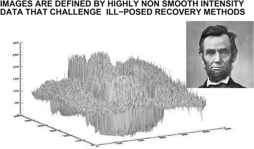
In the backward recovery problems discussed in [18–25], initial values at t = 0 are sought from relatively smooth noisy data at time $T_{max}>0$, data that are known to approximate an actual solution to within a known small $\delta >0,$ in an appropriate ${\mathcal{L}}^p$ norm. In the successful numerical experiments discussed in [18–25], the data at t = 0 are typically chosen to be grey-scale images, defined by highly non smooth intensity data that are not easily synthesized mathematically. An example of such an image is shown in Figure 1 below.

Figure 1. Plot of intensity values $u(x,y)$ versus $(x,y)$ in $512\times 512$ pixel Abraham Lincoln image. Intensity values range from 0 to 255, and result in highly non smooth surface. Such images provide excellent test examples for ill-posed reconstruction methods.

However, the data assimilation problem is fundamentally different from the above backward recovery problem. In the data assimilation case, the target data at time $T_{max}>0$ may not be smooth, may not correspond to an actual solution, and may differ from an actual solution by an unknown large $\delta >0$ in that same ${\mathcal{L}}^p$ norm. Moreover, it may not be possible to find useful initial values at t = 0. Unexpectedly, as shown in [16,17], and as will be shown below, stabilized explicit schemes may sometimes be useful in the data assimilation problem, by using more aggressive smoothing at each time step.

In the present paper, the backward recovery problem in the coupled system discussed in [22] is of particular interest. In [22, Figures 2 and 3], the complex forward evolution of the three independent non negative initial images at $t=0,$ is made evident. In the solution at time $T_{max}=7.5\times {10}^{-3},$ each image displays the influence of the other two images, as well as negative values. Nevertheless, as shown in the last row in Figure 2, successful recovery of the initial data was found possible from the data at $T_{max}$.

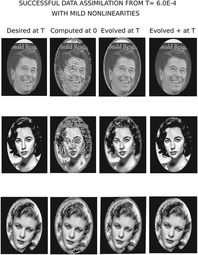
Figure 2. Leftmost column is the hypothetical data $W^{\ast }(\cdot ,T_{max})$. Second column from left is $U(\cdot ,0)$, the backward computation to t = 0, using the hypothetical data at $T_{max}$. Third column from left is the forward evolution at time $T_{max}$, of the computed initial data $U(\cdot ,0)$ at t = 0, shown in previous column. Last column is the result of applying the constraint $0\le z(x,y)\le 255$ to the data in the previous column.

As will now be shown, the stabilized explicit scheme developed in [22] can be useful even in more challenging data assimilation problems. With positive constants $\alpha ,\text{β}$, and with L a linear or nonlinear second order elliptic differential operator in two space variables $(x,y)$, defined on bounded domain Ω in $R^2$ with a smooth boundary $\mathrm{\partial }\mathrm{\Omega }$, the following system will be studied (1) $\begin{array}{rl}& u_t=-\text{β}Lu-\alpha Lv,\\ & v_t=Lw+\alpha Lu,\\ & w_t=-Lv,\\ & u(x,y,0)=f(x,y),v(x,y,0)=g(x,y),w(x,y,0)=h(x,y),\\ & u(x,y,t)=v(x,y,t)=w(x,y,t)=0,(x,y,t)\in \mathrm{\partial }\mathrm{\Omega }\times [0,T_{max}].\end{array}$(1) Given hypothetical or desired data $\left[u^{\ast }\right(\cdot ,T_{max}),v^{\ast }(\cdot ,T_{max}),w^{\ast }(\cdot ,T_{max}\left)\right]$, at an appropriate value of $T_{max}>0$, the following data assimilation problem is discussed: find initial values $\left[u\right(.,0),v(.,0),w(.,0\left)\right]$, that can evolve according to Equation (1(1) $\begin{array}{rl}& u_t=-\text{β}Lu-\alpha Lv,\\ & v_t=Lw+\alpha Lu,\\ & w_t=-Lv,\\ & u(x,y,0)=f(x,y),v(x,y,0)=g(x,y),w(x,y,0)=h(x,y),\\ & u(x,y,t)=v(x,y,t)=w(x,y,t)=0,(x,y,t)\in \mathrm{\partial }\mathrm{\Omega }\times [0,T_{max}].\end{array}$(1) ), into a useful approximation to the desired data at time $T_{max}$. Here, non smooth hypothetical data are considered that may not correspond to an actual solution of Equation (1(1) $\begin{array}{rl}& u_t=-\text{β}Lu-\alpha Lv,\\ & v_t=Lw+\alpha Lu,\\ & w_t=-Lv,\\ & u(x,y,0)=f(x,y),v(x,y,0)=g(x,y),w(x,y,0)=h(x,y),\\ & u(x,y,t)=v(x,y,t)=w(x,y,t)=0,(x,y,t)\in \mathrm{\partial }\mathrm{\Omega }\times [0,T_{max}].\end{array}$(1) ) at time $T_{max}$.

In the simplest linear case with $L=-\mathrm{\Delta },w=\mathrm{\Delta }z,v=z_t,$ the above system corresponds to the thermoelastic plate problem $z_{tt}=-{\mathrm{\Delta }}^{2}z-\alpha \mathrm{\Delta }u,u_t=\text{β}\mathrm{\Delta }u+\alpha \mathrm{\Delta }{z}_t,$ with hinged boundary conditions, $u=z=\mathrm{\Delta }z=0$ on $\mathrm{\partial }\mathrm{\Omega }$. This case has been studied by several authors [27–30], and the solution operator is known to be a holomorphic semigroup.

In the developments below, the principal results from [22] that will be needed will be listed without proof, using notation identical to that used in [22] for the reader's convenience. In Section 2, the linear selfadjoint problem is discussed. In Section 3, Theorems 3.1 and 3.2 establish error estimates for the forward and backward explicit schemes. These estimates imply limitations on the class of problems wherein the explicit scheme may be useful, as shown in Equation (17(17) $\parallel W^{\ast }(\cdot ,T_{max})-U(\cdot ,T_{max}){\parallel }_2\le \delta (1+K_1^2)+K_5(1+K_1).$(17) ) in Section 3.1. Section 4 discusses the use of smoothing operators based on the Laplacian, and leads to Theorems 4.1 and 4.2. Section 5 describes nonlinear data assimilation experiments. Finally, Section 6 offers some concluding remarks.

While there are no new theoretical results in the present paper other than the error estimate in Equation (17(17) $\parallel W^{\ast }(\cdot ,T_{max})-U(\cdot ,T_{max}){\parallel }_2\le \delta (1+K_1^2)+K_5(1+K_1).$(17) ), the unexpected success of stabilized explicit schemes in the more challenging data assimilation problems considered here and in [16,17], is of great interest. The numerical experiments discussed in Section 5 below, together with those in [16,17], invite valuable scientific debate and comparisons with what might be achieved on similar examples, using artificial intelligence methods based on neural networks coupled with machine learning.

2. Linear autonomous selfadjoint L in Equation (1)

In Equation (1(1) $\begin{array}{rl}& u_t=-\text{β}Lu-\alpha Lv,\\ & v_t=Lw+\alpha Lu,\\ & w_t=-Lv,\\ & u(x,y,0)=f(x,y),v(x,y,0)=g(x,y),w(x,y,0)=h(x,y),\\ & u(x,y,t)=v(x,y,t)=w(x,y,t)=0,(x,y,t)\in \mathrm{\partial }\mathrm{\Omega }\times [0,T_{max}].\end{array}$(1) ), let <, > and $\parallel {\parallel }_2$, respectively denote the scalar product and norm on ${\mathcal{L}}^2\left(\mathrm{\Omega }\right)$ and let L denote a linear, second order, time-independent, positive definite selfadjoint variable coefficient elliptic differential operator in Ω, with homogeneous Dirichlet boundary conditions on $\mathrm{\partial }\mathrm{\Omega }$. Let $\{{\varphi }_m{\}}_{m=1}^{\mathrm{\infty }}$, be the complete set of orthonormal eigenfunctions for L on Ω, and let $\{{\lambda }_m{\}}_{m=1}^{\mathrm{\infty }}$, satisfying (2) $0<{\lambda }_1\le {\lambda }_2\le \cdots \le {\lambda }_m\le \cdots \uparrow \mathrm{\infty },$(2) be the corresponding eigenvalues.

The initial value problem Equation (1(1) $\begin{array}{rl}& u_t=-\text{β}Lu-\alpha Lv,\\ & v_t=Lw+\alpha Lu,\\ & w_t=-Lv,\\ & u(x,y,0)=f(x,y),v(x,y,0)=g(x,y),w(x,y,0)=h(x,y),\\ & u(x,y,t)=v(x,y,t)=w(x,y,t)=0,(x,y,t)\in \mathrm{\partial }\mathrm{\Omega }\times [0,T_{max}].\end{array}$(1) ) becomes ill-posed when the time direction is reversed. Such time-reversed computations are contemplated by allowing for possible negative time steps $\mathrm{\Delta }t$ in the explicit difference scheme Equation (8(8) $U^{n+1}=S{U}^n+\mathrm{\Delta }tSG{U}^n\equiv R{U}^n,n=0,1,\dots (N-1),U^0=[f,g,h{]}^T.$(8) ) below. With ${\lambda }_m$ as in Equation (2(2) $0<{\lambda }_1\le {\lambda }_2\le \cdots \le {\lambda }_m\le \cdots \uparrow \mathrm{\infty },$(2) ), the positive constants $\alpha ,\text{β}$ and the operator L as in Equation (1(1) $\begin{array}{rl}& u_t=-\text{β}Lu-\alpha Lv,\\ & v_t=Lw+\alpha Lu,\\ & w_t=-Lv,\\ & u(x,y,0)=f(x,y),v(x,y,0)=g(x,y),w(x,y,0)=h(x,y),\\ & u(x,y,t)=v(x,y,t)=w(x,y,t)=0,(x,y,t)\in \mathrm{\partial }\mathrm{\Omega }\times [0,T_{max}].\end{array}$(1) ), fix $\omega >0$ and p>1. Given $\mathrm{\Delta }t$, define $\nu ,\mathrm{\Lambda },Q,{\zeta }_m,r_m$, as follows: (3) $\begin{array}{rl}& \nu =(3+\alpha +{\alpha }^2+2\text{β}),\mathrm{\Lambda }=\nu (I+L),Q=\exp (-\omega |\mathrm{\Delta }t|{\mathrm{\Lambda }}^p),\\ & {\zeta }_m=\nu (1+{\lambda }_m)>3,r_m=\exp (-\omega |\mathrm{\Delta }t|({\zeta }_m{)}^p),m\ge 1.\end{array}$(3) In the present discussion, the family $\{{\lambda }_m,{\varphi }_m\}$ in Equation (2(2) $0<{\lambda }_1\le {\lambda }_2\le \cdots \le {\lambda }_m\le \cdots \uparrow \mathrm{\infty },$(2) ), is assumed known or precomputed. However, as will be illustrated below, in many practical computations, a different smoothing operator, based on a substitute elliptic operator $L^{†}$ with known characteristic pairs, such as the negative Laplacian, can be used instead. Since p>1 has non integer values typically, both the operators ${\mathrm{\Lambda }}^p$ and Q in Equation (3(3) $\begin{array}{rl}& \nu =(3+\alpha +{\alpha }^2+2\text{β}),\mathrm{\Lambda }=\nu (I+L),Q=\exp (-\omega |\mathrm{\Delta }t|{\mathrm{\Lambda }}^p),\\ & {\zeta }_m=\nu (1+{\lambda }_m)>3,r_m=\exp (-\omega |\mathrm{\Delta }t|({\zeta }_m{)}^p),m\ge 1.\end{array}$(3) ), must be synthesized in terms of the characteristic pairs $\{{\lambda }_m,{\varphi }_m\}$ of L. With ${\zeta }_m,r_m$ as in Equation (3(3) $\begin{array}{rl}& \nu =(3+\alpha +{\alpha }^2+2\text{β}),\mathrm{\Lambda }=\nu (I+L),Q=\exp (-\omega |\mathrm{\Delta }t|{\mathrm{\Lambda }}^p),\\ & {\zeta }_m=\nu (1+{\lambda }_m)>3,r_m=\exp (-\omega |\mathrm{\Delta }t|({\zeta }_m{)}^p),m\ge 1.\end{array}$(3) ), define for every $h\in {\mathcal{L}}^2\left(\mathrm{\Omega }\right)$, (4) ${\mathrm{\Lambda }}^{p}h={\mathrm{\Sigma }}_{m=1}^{\mathrm{\infty }}({\zeta }_m{)}^p<h,{\varphi }_m>{\varphi }_m,Qh={\mathrm{\Sigma }}_{m=1}^{\mathrm{\infty }}{r}_m<h,{\varphi }_m>{\varphi }_m.$(4) Let G, S, and P, be the following $3\times 3$ matrices (5) $G=\left[\begin{array}{ccc}-\text{β}L& -\alpha L& 0\\ \alpha L& 0& L\\ 0& -L& 0\end{array}\right],S=\left[\begin{array}{ccc}Q& 0& 0\\ 0& Q& 0\\ 0& 0& Q\end{array}\right],P=\left[\begin{array}{ccc}{\mathrm{\Lambda }}^p& 0& 0\\ 0& {\mathrm{\Lambda }}^p& 0\\ 0& 0& {\mathrm{\Lambda }}^p\end{array}\right].$(5) Let W be the three component vector $[u,v,w{]}^T$. We may rewrite Equation (1(1) $\begin{array}{rl}& u_t=-\text{β}Lu-\alpha Lv,\\ & v_t=Lw+\alpha Lu,\\ & w_t=-Lv,\\ & u(x,y,0)=f(x,y),v(x,y,0)=g(x,y),w(x,y,0)=h(x,y),\\ & u(x,y,t)=v(x,y,t)=w(x,y,t)=0,(x,y,t)\in \mathrm{\partial }\mathrm{\Omega }\times [0,T_{max}].\end{array}$(1) ) as the equivalent first order system, (6) $W_t=GW,0<t\le T_{max},W(\cdot ,0)=[f,g,h{]}^T.$(6) An explicit time-marching finite difference scheme will be studied for Equation (6(6) $W_t=GW,0<t\le T_{max},W(\cdot ,0)=[f,g,h{]}^T.$(6) ), in which only the time variable is discretized, while the space variables remain continuous. With a given positive integer N, let $|\mathrm{\Delta }t|=T_{max}/N$ be the time step magnitude, and let $W^n$ denote $W(\cdot ,n\mathrm{\Delta }t),n=0,1,\dots N$. If $W(\cdot ,t)$ is the unique solution of Equation (6(6) $W_t=GW,0<t\le T_{max},W(\cdot ,0)=[f,g,h{]}^T.$(6) ), then (7) $W^{n+1}=W^n+\mathrm{\Delta }tG{W}^n+{\tau }^n,$(7) where the ‘truncation error’ ${\tau }^n=\frac{1}{2}\left(\mathrm{\Delta }t{)}^2{G}^{2}W\right(\cdot ,\tilde{t})$, with $n|\mathrm{\Delta }t|<\tilde{t}<(n+1)|\mathrm{\Delta }t|$. With G and S as in Equation (5(5) $G=\left[\begin{array}{ccc}-\text{β}L& -\alpha L& 0\\ \alpha L& 0& L\\ 0& -L& 0\end{array}\right],S=\left[\begin{array}{ccc}Q& 0& 0\\ 0& Q& 0\\ 0& 0& Q\end{array}\right],P=\left[\begin{array}{ccc}{\mathrm{\Lambda }}^p& 0& 0\\ 0& {\mathrm{\Lambda }}^p& 0\\ 0& 0& {\mathrm{\Lambda }}^p\end{array}\right].$(5) ), let R be the linear operator $R=S+\mathrm{\Delta }tSG$. Using the smoothing operator S, we consider approximating $W^n$ with $U^n\equiv [u^n,v^n,w^n{]}^T$, where (8) $U^{n+1}=S{U}^n+\mathrm{\Delta }tSG{U}^n\equiv R{U}^n,n=0,1,\dots (N-1),U^0=[f,g,h{]}^T.$(8) With $\mathrm{\Delta }t>0$ and the data $U^0$ at time t = 0, the forward marching scheme in Equation (8(8) $U^{n+1}=S{U}^n+\mathrm{\Delta }tSG{U}^n\equiv R{U}^n,n=0,1,\dots (N-1),U^0=[f,g,h{]}^T.$(8) ) aims to solve a well-posed problem. However, with $\mathrm{\Delta }t<0$, together with appropriate data $U^0$ at time $T_{max}$, marching backward from $T_{max}$ in Equation (8(8) $U^{n+1}=S{U}^n+\mathrm{\Delta }tSG{U}^n\equiv R{U}^n,n=0,1,\dots (N-1),U^0=[f,g,h{]}^T.$(8) ) attempts to solve an ill-posed problem. It remains to be seen whether $U^n$ can be a useful approximation to $W^n$, by proper choices of $\omega ,p$, and $|\mathrm{\Delta }t|$. Define the following norms for three component vectors such as $W(\cdot ,t)$ and $U^n$, (9) $\begin{array}{rl}\parallel W(\cdot ,t){\parallel }_2& ={\{\parallel u(\cdot ,t){\parallel }_2^2+\parallel v(\cdot ,t){\parallel }_2^2+\parallel w(\cdot ,t\left){\parallel }_2^2\right\}}^{1/2},\\ \parallel U^n{\parallel }_2& ={\{\parallel u^n{\parallel }_2^2+\parallel v^n{\parallel }_2^2+\parallel w^n{\parallel }_2^2\}}^{1/2},\\ |||W||{|}_{2,\mathrm{\infty }}& =\underset{0\le t\le T_{max}}{sup}\{\parallel W(\cdot ,t\left){\parallel }_2\right\}.\end{array}$(9) Lemma 2.1 below is proved in [22].

Lemma 2.1

With p>1, and ${\zeta }_m,r_m,$ as in Equation (3(3) $\begin{array}{rl}& \nu =(3+\alpha +{\alpha }^2+2\text{β}),\mathrm{\Lambda }=\nu (I+L),Q=\exp (-\omega |\mathrm{\Delta }t|{\mathrm{\Lambda }}^p),\\ & {\zeta }_m=\nu (1+{\lambda }_m)>3,r_m=\exp (-\omega |\mathrm{\Delta }t|({\zeta }_m{)}^p),m\ge 1.\end{array}$(3) ), fix a positive integer J, and choose $\omega \ge ({\zeta }_J{)}^{1-p}$. Then, (10) $r_m(1+|\mathrm{\Delta }t|{\zeta }_m)\le 1+|\mathrm{\Delta }t|{\zeta }_J,m\ge 1.$(10)

3. Error estimates and stabilization penalties

Explicit time differencing in systems of partial differential involving heat conduction, generally requires stringent Courant stability restrictions on the time step $\mathrm{\Delta }t$. The stabilizing smoothing operator S in the explicit scheme in Equation (8(8) $U^{n+1}=S{U}^n+\mathrm{\Delta }tSG{U}^n\equiv R{U}^n,n=0,1,\dots (N-1),U^0=[f,g,h{]}^T.$(8) ) leads to unconditional stability, but at the cost of introducing a small error at each time step. If the accumulated error at the final time $T_{max}$ is sufficiently small, the stabilized explicit scheme would offer considerable advantages in the computation of multidimensional problems on fine meshes. Theorems 3.1 and 3.2 below are proved in [22].

Theorem 3.1

With $\mathrm{\Delta }t>0$, let $W^n$ be the unique solution of Equation (6(6) $W_t=GW,0<t\le T_{max},W(\cdot ,0)=[f,g,h{]}^T.$(6) ) at $t=n\mathrm{\Delta }t$. Let $U^n$ be the corresponding solution of the forward explicit scheme in Equation (8(8) $U^{n+1}=S{U}^n+\mathrm{\Delta }tSG{U}^n\equiv R{U}^n,n=0,1,\dots (N-1),U^0=[f,g,h{]}^T.$(8) ), and let $p,{\zeta }_J,\omega ,$ be as in Lemma 2.1. If $Z\left(t\right)\equiv U^n-W^n,$ denotes the error at $t=n\mathrm{\Delta }t,n=0,1,2,\dots ,N,$ we have (11) $\begin{array}{rl}& \parallel Z\left(t\right){\parallel }_2\le {\mathrm{e}}^{t{\zeta }_J}\parallel Z\left(0\right){\parallel }_2+\left\{\omega \right({\mathrm{e}}^{t{\zeta }_J}-1\left)/{\zeta }_J\right\}|||PW||{|}_{2,\mathrm{\infty }}\\ & +\left\{\right({\mathrm{e}}^{t{\zeta }_J}-1\left)/{\zeta }_J\right\}\{\omega \mathrm{\Delta }t|||PGW||{|}_{2,\mathrm{\infty }}+(\mathrm{\Delta }t/2\left)|||G^{2}W||{|}_{2,\mathrm{\infty }}\right\}.\end{array}$(11)

In the forward problem, as $\mathrm{\Delta }t\downarrow 0,$ we are left with the error originating in the possibly erroneous initial data $U^0=[f,g,h{]}^T$, together with the stabilization penalty represented by the second term in Equation (11(11) $\begin{array}{rl}& \parallel Z\left(t\right){\parallel }_2\le {\mathrm{e}}^{t{\zeta }_J}\parallel Z\left(0\right){\parallel }_2+\left\{\omega \right({\mathrm{e}}^{t{\zeta }_J}-1\left)/{\zeta }_J\right\}|||PW||{|}_{2,\mathrm{\infty }}\\ & +\left\{\right({\mathrm{e}}^{t{\zeta }_J}-1\left)/{\zeta }_J\right\}\{\omega \mathrm{\Delta }t|||PGW||{|}_{2,\mathrm{\infty }}+(\mathrm{\Delta }t/2\left)|||G^{2}W||{|}_{2,\mathrm{\infty }}\right\}.\end{array}$(11) ). These errors grow monotonically as $t\uparrow T_{max}$. Clearly, if $T_{max}$ is large, the accumulated distortion may become unacceptably large as $t\uparrow T_{max}$, and the stabilized explicit scheme is not useful in that case.

Marching backward from $t=T_{max}$ in the backward problem, solutions exist only for a restricted class of data satisfying certain smoothness constraints. Such data are seldom known with sufficient accuracy. This is especially true of the hypothetical data $W^{\ast }(\cdot ,T_{max})$ in the present data assimilation problem. It will be assumed that the given data $W^{\ast }(\cdot ,T_{max})$, differ from the necessary exact data $W(\cdot ,T_{max})$, by an unknown amount δ in the ${\mathcal{L}}^2\left(\mathrm{\Omega }\right)$ norm. (12) $\parallel W^{\ast }(\cdot ,T_{max})-W(\cdot ,T_{max}){\parallel }_2\le \delta .$(12) This leads to the following result.

Theorem 3.2

With $\mathrm{\Delta }t<0$, let $W^n$ be the unique solution of the forward well-posed problem in Equation (6(6) $W_t=GW,0<t\le T_{max},W(\cdot ,0)=[f,g,h{]}^T.$(6) ) at $s=T_{max}-n|\mathrm{\Delta }t|$. Let $U^n$ be the solution of the backward explicit scheme in Equation (8(8) $U^{n+1}=S{U}^n+\mathrm{\Delta }tSG{U}^n\equiv R{U}^n,n=0,1,\dots (N-1),U^0=[f,g,h{]}^T.$(8) ), with initial data $U\left(0\right)=W^{\ast }(\cdot ,T_{max})$, as in Equation (12(12) $\parallel W^{\ast }(\cdot ,T_{max})-W(\cdot ,T_{max}){\parallel }_2\le \delta .$(12) ). Let $p,{\zeta }_J,\omega ,$ be as in Lemma 2.1. If $Z\left(s\right)\equiv U^n-W^n,$ denotes the error at $s=T_{max}-n|\mathrm{\Delta }t|,n=0,1,2,\dots ,N,$ we have, with δ as in Equation (12(12) $\parallel W^{\ast }(\cdot ,T_{max})-W(\cdot ,T_{max}){\parallel }_2\le \delta .$(12) ), (13) $\begin{array}{rl}& \parallel Z\left(s\right){\parallel }_2\le \delta {\mathrm{e}}^{n|\mathrm{\Delta }t|{\zeta }_J}+\left\{\omega \right({\mathrm{e}}^{n|\mathrm{\Delta }t|{\zeta }_J}-1\left)/{\zeta }_J\right\}|||PW||{|}_{2,\mathrm{\infty }}\\ & +\left\{\right({\mathrm{e}}^{n|\mathrm{\Delta }t|{\zeta }_J}-1\left)/{\zeta }_J\right\}\{\omega |\mathrm{\Delta }t||||PGW||{|}_{2,\mathrm{\infty }}+(|\mathrm{\Delta }t|/2\left)|||G^{2}W||{|}_{2,\mathrm{\infty }}\right\}.\end{array}$(13)

3.1. Application to data assimilation

In Theorems 3.1 and 3.2 above, define the constants $K_1$ through $K_5$ as follows, and consider the values shown in Table 1 below. (14) $\begin{array}{rl}& K_1={\mathrm{e}}^{{\zeta }_J{T}_{max}},K_2=\omega ({\mathrm{e}}^{{\zeta }_J{T}_{max}}-1)/{\zeta }_J,K_3=|\mathrm{\Delta }t|K_2,K_4=K_3/\left(2\omega \right),\\ & K_5=K_2|||PW||{|}_{2,\mathrm{\infty }}+K_3|||PGW||{|}_{2,\mathrm{\infty }}+K_4|||G^{2}W||{|}_{2,\mathrm{\infty }}.\end{array}$(14)

Table 1. Values of $K_1$ through $K_4$ in Equation (14(14) $\begin{array}{rl}& K_1={\mathrm{e}}^{{\zeta }_J{T}_{max}},K_2=\omega ({\mathrm{e}}^{{\zeta }_J{T}_{max}}-1)/{\zeta }_J,K_3=|\mathrm{\Delta }t|K_2,K_4=K_3/\left(2\omega \right),\\ & K_5=K_2|||PW||{|}_{2,\mathrm{\infty }}+K_3|||PGW||{|}_{2,\mathrm{\infty }}+K_4|||G^{2}W||{|}_{2,\mathrm{\infty }}.\end{array}$(14) ), with following parameter values: $T_{max}=6\times {10}^{-4},|\mathrm{\Delta }t|=3\times {10}^{-7},p=3.5,{\zeta }_J=3017,\omega ={\zeta }_J^{(1-p)}=2\times {10}^{-9}$.

$K_1={\mathrm{e}}^{{\zeta }_J{T}_{max}}$	$K_2=\left({\zeta }_J{)}^{-p}\right(K_1-1)$	$K_3=\left|\mathrm{\Delta }t\right|K_2$	$K_4=K_3/\left(2\omega \right)$
$K_1<6.2$	$K_2<3.5\times {10}^{-12}$	$K_3<1.1\times {10}^{-18}$	$K_4<2.8\times {10}^{-10}$

As outlined in the Introduction, data assimilation applied to the system in Equation (1(1) $\begin{array}{rl}& u_t=-\text{β}Lu-\alpha Lv,\\ & v_t=Lw+\alpha Lu,\\ & w_t=-Lv,\\ & u(x,y,0)=f(x,y),v(x,y,0)=g(x,y),w(x,y,0)=h(x,y),\\ & u(x,y,t)=v(x,y,t)=w(x,y,t)=0,(x,y,t)\in \mathrm{\partial }\mathrm{\Omega }\times [0,T_{max}].\end{array}$(1) ), is the problem of finding initial values $\left[u\right(.,0),v(.,0),w(.,0\left)\right]$, at t = 0, that can evolve into useful approximations to $W^{\ast }(\cdot ,T_{max})$, the given hypothetical data at an appropriate time $T_{max}>0$. If the true solution in Equation (1(1) $\begin{array}{rl}& u_t=-\text{β}Lu-\alpha Lv,\\ & v_t=Lw+\alpha Lu,\\ & w_t=-Lv,\\ & u(x,y,0)=f(x,y),v(x,y,0)=g(x,y),w(x,y,0)=h(x,y),\\ & u(x,y,t)=v(x,y,t)=w(x,y,t)=0,(x,y,t)\in \mathrm{\partial }\mathrm{\Omega }\times [0,T_{max}].\end{array}$(1) ) does not have exceedingly large values for $|||PW||{|}_{2,\mathrm{\infty }},|||PGW||{|}_{2,\mathrm{\infty }}$, or $|||G^{2}W||{|}_{2,\mathrm{\infty }}$, the parameter values chosen in Table 1, together with Theorem 3.2, indicate that marching backward to time t = 0 from the hypothetical data $W^{\ast }$ at $T_{max}$, leads to an error $Z\left(0\right)$, satisfying (15) $\parallel Z\left(0\right){\parallel }_2\le \delta K_1+K_5,$(15) with the constant $K_5$ defined in Equation (14(14) $\begin{array}{rl}& K_1={\mathrm{e}}^{{\zeta }_J{T}_{max}},K_2=\omega ({\mathrm{e}}^{{\zeta }_J{T}_{max}}-1)/{\zeta }_J,K_3=|\mathrm{\Delta }t|K_2,K_4=K_3/\left(2\omega \right),\\ & K_5=K_2|||PW||{|}_{2,\mathrm{\infty }}+K_3|||PGW||{|}_{2,\mathrm{\infty }}+K_4|||G^{2}W||{|}_{2,\mathrm{\infty }}.\end{array}$(14) ) presumed small. Next, from Theorem 3.1, marching forward to time $T_{max}$ using the inexact computed initial values $U(\cdot ,0)$, leads to an error $Z\left(T_{max}\right)$, satisfying (16) $\parallel Z\left(T_{max}\right){\parallel }_2\le K_1(\delta K_1+K_5)+K_5.$(16) The error $Z\left(T_{max}\right)$ in Theorem 3.1 is the difference at time $T_{max}$, between the unknown unique solution $W(\cdot ,t)$ in Equation (6(6) $W_t=GW,0<t\le T_{max},W(\cdot ,0)=[f,g,h{]}^T.$(6) ), and the computed numerical approximation to it, $U(\cdot ,t)$, provided by the stabilized forward explicit scheme. However, $\parallel W^{\ast }(\cdot ,T_{max})-W(\cdot ,(T_{max}){\parallel }_2\le \delta$, if $W^{\ast }(\cdot ,T_{max})$ is the given hypothetical data. Hence, using the triangle inequality, we find (17) $\parallel W^{\ast }(\cdot ,T_{max})-U(\cdot ,T_{max}){\parallel }_2\le \delta (1+K_1^2)+K_5(1+K_1).$(17) Therefore, data assimilation is successful only if the inexact computed initial values $U(\cdot ,0)$ at t = 0, lead to a sufficiently small right hand side in Equation (17(17) $\parallel W^{\ast }(\cdot ,T_{max})-U(\cdot ,T_{max}){\parallel }_2\le \delta (1+K_1^2)+K_5(1+K_1).$(17) ). Clearly, the value of ${\zeta }_J{T}_{max}$, together with the unknown value of δ, will play a vital role.

4. Using the Laplacian for smoothing when L has variable coefficients

As previously noted, the developments in Sections 2 and 3 presuppose knowledge of the characteristic pairs of the variable coefficient elliptic operator L, or the precomputation of a sufficiently large number of such pairs. However, it is often possible to use a substitute smoothing operator $Q^{†},$ based on a different elliptic operator with known characteristic pairs.

Let Δ denote the Laplacian operator in Ω, with homogeneous Dirichlet boundary conditions on $\mathrm{\partial }\mathrm{\Omega }$. With $\nu ,L,\mathrm{\Lambda },$ as in Equation (3(3) $\begin{array}{rl}& \nu =(3+\alpha +{\alpha }^2+2\text{β}),\mathrm{\Lambda }=\nu (I+L),Q=\exp (-\omega |\mathrm{\Delta }t|{\mathrm{\Lambda }}^p),\\ & {\zeta }_m=\nu (1+{\lambda }_m)>3,r_m=\exp (-\omega |\mathrm{\Delta }t|({\zeta }_m{)}^p),m\ge 1.\end{array}$(3) ), let $\mathrm{\Gamma }=\nu (I-\mathrm{\Delta })$. For any real q>1 and $ϵ>0,$ define (18) $Q_{\mathrm{\Delta }}=\exp \{-ϵ|\mathrm{\Delta }t|{\mathrm{\Gamma }}^q\},$(18) Closed form expressions for the eigenfunctions of the Laplacian are known for specific domains that are important in applications, including rectangles, circles, and spheres [31]. On such domains, it may be advantageous to construct smoothing operators $Q_{\mathrm{\Delta }}$ based on the Laplacian, in lieu of the smoothing operator Q in Equation (3(3) $\begin{array}{rl}& \nu =(3+\alpha +{\alpha }^2+2\text{β}),\mathrm{\Lambda }=\nu (I+L),Q=\exp (-\omega |\mathrm{\Delta }t|{\mathrm{\Lambda }}^p),\\ & {\zeta }_m=\nu (1+{\lambda }_m)>3,r_m=\exp (-\omega |\mathrm{\Delta }t|({\zeta }_m{)}^p),m\ge 1.\end{array}$(3) ). Such a program is feasible for those differential operators L for which the following result is valid: Given any $\omega >0$, and $p>1,$ there exist $ϵ>0,$ and real $q\ge p,$ such that for all $g\in {\mathcal{L}}^2\left(\mathrm{\Omega }\right)$ and sufficiently small $|\mathrm{\Delta }t|,$ (19) $\parallel \exp \{-ϵ|\mathrm{\Delta }t|{\mathrm{\Gamma }}^q\}g{\parallel }_2\le \parallel \exp \{-\omega |\mathrm{\Delta }t|{\mathrm{\Lambda }}^p\}g{\parallel }_2,⟺\parallel Q_{\mathrm{\Delta }}g{\parallel }_2\le \parallel Qg{\parallel }_2.$(19) The linear operator $H=(\exp \{-ϵ|\mathrm{\Delta }t|{\mathrm{\Gamma }}^q\left\}\right)(\exp \{\omega |\mathrm{\Delta }t|{\mathrm{\Lambda }}^p\left\}\right)$ is well-defined on the range of $(\exp \{-\omega |\mathrm{\Delta }t|{\mathrm{\Lambda }}^p\left\}\right)$, which is dense in ${\mathcal{L}}^2\left(\mathrm{\Omega }\right)$. The inequality in Equation (19(19) $\parallel \exp \{-ϵ|\mathrm{\Delta }t|{\mathrm{\Gamma }}^q\}g{\parallel }_2\le \parallel \exp \{-\omega |\mathrm{\Delta }t|{\mathrm{\Lambda }}^p\}g{\parallel }_2,⟺\parallel Q_{\mathrm{\Delta }}g{\parallel }_2\le \parallel Qg{\parallel }_2.$(19) ) would follow if it can be shown that H can be extended to a bounded operator on all of ${\mathcal{L}}^2\left(\mathrm{\Omega }\right)$, with $\parallel H{\parallel }_2\le 1$.

Equation (19(19) $\parallel \exp \{-ϵ|\mathrm{\Delta }t|{\mathrm{\Gamma }}^q\}g{\parallel }_2\le \parallel \exp \{-\omega |\mathrm{\Delta }t|{\mathrm{\Lambda }}^p\}g{\parallel }_2,⟺\parallel Q_{\mathrm{\Delta }}g{\parallel }_2\le \parallel Qg{\parallel }_2.$(19) ) appears to be validated in numerous computational experiments. Results of a somewhat similar nature are known in the theory of Gaussian estimates for heat kernels. See e.g. [32–35], and the references therein.

Let $S_{\mathrm{\Delta }}$ and $P_{\mathrm{\Delta }}$ be the following $3\times 3$ matrices (20) $S_{\mathrm{\Delta }}=\left[\begin{array}{ccc}{Q}_{\mathrm{\Delta }}& 0& 0\\ 0& Q_{\mathrm{\Delta }}& 0\\ 0& 0& Q_{\mathrm{\Delta }}\end{array}\right],P_{\mathrm{\Delta }}=\left[\begin{array}{ccc}{\mathrm{\Gamma }}^q& 0& 0\\ 0& {\mathrm{\Gamma }}^q& 0\\ 0& 0& {\mathrm{\Gamma }}^q\end{array}\right].$(20) The Laplacian stabilized explicit scheme corresponding to Equation (8(8) $U^{n+1}=S{U}^n+\mathrm{\Delta }tSG{U}^n\equiv R{U}^n,n=0,1,\dots (N-1),U^0=[f,g,h{]}^T.$(8) ) is given by (21) $U^{n+1}=S_{\mathrm{\Delta }}{U}^n+\mathrm{\Delta }t{S}_{\mathrm{\Delta }}G{U}^n\equiv R_{\mathrm{\Delta }}{U}^n,n=0,1,\dots (N-1),U^0=[f,g,h{]}^T,$(21)

Remark 4.1

Useful pairs $(ϵ,q)$ in the Laplacian stabilized scheme in Equation (21(21) $U^{n+1}=S_{\mathrm{\Delta }}{U}^n+\mathrm{\Delta }t{S}_{\mathrm{\Delta }}G{U}^n\equiv R_{\mathrm{\Delta }}{U}^n,n=0,1,\dots (N-1),U^0=[f,g,h{]}^T,$(21) ) are generally found interactively after relatively few trials. In many data assimilation experiments, typical values satisfy $2<q<4,{10}^{-10}\le ϵ\le {10}^{-6}.$

Theorem 4.1

Let $p,{\zeta }_J,\omega ,$ be as in Lemma 2.1, and choose $ϵ>0$ and $q\ge p$, such that Equation (19(19) $\parallel \exp \{-ϵ|\mathrm{\Delta }t|{\mathrm{\Gamma }}^q\}g{\parallel }_2\le \parallel \exp \{-\omega |\mathrm{\Delta }t|{\mathrm{\Lambda }}^p\}g{\parallel }_2,⟺\parallel Q_{\mathrm{\Delta }}g{\parallel }_2\le \parallel Qg{\parallel }_2.$(19) ) is satisfied. With $\mathrm{\Delta }t>0$, let $W^n$ be the unique solution of Equation (6(6) $W_t=GW,0<t\le T_{max},W(\cdot ,0)=[f,g,h{]}^T.$(6) ) at $t=n\mathrm{\Delta }t$, and let $U^n$ be the corresponding solution of the forward explicit scheme in Equation (21(21) $U^{n+1}=S_{\mathrm{\Delta }}{U}^n+\mathrm{\Delta }t{S}_{\mathrm{\Delta }}G{U}^n\equiv R_{\mathrm{\Delta }}{U}^n,n=0,1,\dots (N-1),U^0=[f,g,h{]}^T,$(21) ). If $Z_{\mathrm{\Delta }}\left(t\right)\equiv U^n-W^n,$ denotes the error at $t=n\mathrm{\Delta }t,n=0,1,2,\dots ,N,$ then (22) $\begin{array}{rl}\parallel Z_{\mathrm{\Delta }}\left(t\right){\parallel }_2& \le {\mathrm{e}}^{t{\zeta }_J}\parallel Z_{\mathrm{\Delta }}\left(0\right){\parallel }_2+\left\{ϵ\right({\mathrm{e}}^{t{\zeta }_J}-1\left)/{\zeta }_J\right\}|||P_{\mathrm{\Delta }}W||{|}_{2,\mathrm{\infty }}\\ & +\left\{\right({\mathrm{e}}^{t{\zeta }_J}-1\left)/{\zeta }_J\right\}\{ϵ\mathrm{\Delta }t|||P_{\mathrm{\Delta }}GW||{|}_{2,\mathrm{\infty }}+(\mathrm{\Delta }t/2\left)|||G^{2}W||{|}_{2,\mathrm{\infty }}\right\}.\end{array}$(22)

Theorem 4.2

Let $p,{\zeta }_J,\omega ,$ be as in Lemma 2.1, and choose $ϵ>0$ and $q\ge p$, such that Equation (19(19) $\parallel \exp \{-ϵ|\mathrm{\Delta }t|{\mathrm{\Gamma }}^q\}g{\parallel }_2\le \parallel \exp \{-\omega |\mathrm{\Delta }t|{\mathrm{\Lambda }}^p\}g{\parallel }_2,⟺\parallel Q_{\mathrm{\Delta }}g{\parallel }_2\le \parallel Qg{\parallel }_2.$(19) ) is satisfied. With $\mathrm{\Delta }t<0$, let $W^n$ be the unique solution of the forward well-posed problem in Equation (6(6) $W_t=GW,0<t\le T_{max},W(\cdot ,0)=[f,g,h{]}^T.$(6) ) at $s=T_{max}-n|\mathrm{\Delta }t|$. Let $U^n$ be the solution of the backward explicit scheme in Equation (21(21) $U^{n+1}=S_{\mathrm{\Delta }}{U}^n+\mathrm{\Delta }t{S}_{\mathrm{\Delta }}G{U}^n\equiv R_{\mathrm{\Delta }}{U}^n,n=0,1,\dots (N-1),U^0=[f,g,h{]}^T,$(21) ), with initial data $U\left(0\right)=W^{\ast }(\cdot ,T_{max})$ as in Equation (12(12) $\parallel W^{\ast }(\cdot ,T_{max})-W(\cdot ,T_{max}){\parallel }_2\le \delta .$(12) ). If $Z_{\mathrm{\Delta }}\left(s\right)\equiv U^n-W^n,$ denotes the error at $s=T_{max}-n|\mathrm{\Delta }t|,n=0,1,2,\dots ,N,$ we have, with δ as in Equation (12(12) $\parallel W^{\ast }(\cdot ,T_{max})-W(\cdot ,T_{max}){\parallel }_2\le \delta .$(12) ), (23) $\begin{array}{rl}\parallel Z_{\mathrm{\Delta }}\left(s\right){\parallel }_2& \le \delta {\mathrm{e}}^{n|\mathrm{\Delta }t|{\zeta }_J}+\left\{ϵ\right({\mathrm{e}}^{n|\mathrm{\Delta }t|{\zeta }_J}-1\left)/{\zeta }_J\right\}|||P_{\mathrm{\Delta }}W||{|}_{2,\mathrm{\infty }}\\ & +\left\{\right({\mathrm{e}}^{n|\mathrm{\Delta }t|{\zeta }_J}-1\left)/{\zeta }_J\right\}\{ϵ|\mathrm{\Delta }t||||P_{\mathrm{\Delta }}GW||{|}_{2,\mathrm{\infty }}+(|\mathrm{\Delta }t|/2\left)|||G^{2}W||{|}_{2,\mathrm{\infty }}\right\}.\end{array}$(23)

Remark 4.2

In rectangular regions, the Fast Fourier Transform is an efficient tool for synthesizing ${\mathrm{\Gamma }}^q$ for positive non-integer q, when $\mathrm{\Gamma }=\nu (I-\mathrm{\Delta })$. In [22, Section 6.1], an approach to the use of FFT Laplacian smoothing in non rectangular regions is discussed, and that approach is the one used in the numerical experiments described below.

5. Nonlinear computational experiments with FFT Laplacian smoothing

While the theoretical developments in Sections 2, 3, and 4, are restricted to linear, autonomous, selfadjoint elliptic operators L, the stabilized scheme in Equation (21(21) $U^{n+1}=S_{\mathrm{\Delta }}{U}^n+\mathrm{\Delta }t{S}_{\mathrm{\Delta }}G{U}^n\equiv R_{\mathrm{\Delta }}{U}^n,n=0,1,\dots (N-1),U^0=[f,g,h{]}^T,$(21) ) may be applied to more general problems. Let Ω be the open elliptical region in the $(x,y)$ plane, defined by (24) $0<x,y<1,2.75(x-0.5{)}^2+1.75(y-0.5{)}^2\le 1.$(24) Let L be the nonlinear differential operator defined as follows on functions $z(x,y,t)$ on $\mathrm{\Omega }\times (0,T_{max})$: (25) $Lz=-0.001s\left(z\right)\mathrm{\nabla }.\left\{q\right(x,y,t\left)\mathrm{\nabla }z\right\}-\gamma (z{z}_x+z{z}_y),$(25) where (26) $\begin{array}{rl}s\left(z\right)& =\exp \left\{0.0075\sqrt{|z]}\right\},\gamma =0.01,\\ q(x,y,t)& =\exp \left(10t\right)\{1+2\sin \pi x\sin \pi y\}\ge 1.\end{array}$(26) With $\alpha =\text{β}=3,$ and $(x,y,t)\in \mathrm{\Omega }\times (0,T_{max})$, we now consider the system described in Equation (1(1) $\begin{array}{rl}& u_t=-\text{β}Lu-\alpha Lv,\\ & v_t=Lw+\alpha Lu,\\ & w_t=-Lv,\\ & u(x,y,0)=f(x,y),v(x,y,0)=g(x,y),w(x,y,0)=h(x,y),\\ & u(x,y,t)=v(x,y,t)=w(x,y,t)=0,(x,y,t)\in \mathrm{\partial }\mathrm{\Omega }\times [0,T_{max}].\end{array}$(1) ). Such a system differs from that considered in Section 2, in that the operator L in Equation (25(25) $Lz=-0.001s\left(z\right)\mathrm{\nabla }.\left\{q\right(x,y,t\left)\mathrm{\nabla }z\right\}-\gamma (z{z}_x+z{z}_y),$(25) ) is nonlinear, time-dependent, and non-selfadjoint. Therefore, the theoretical developments in Sections 2, 3, and 4, do not apply to Equation (1(1) $\begin{array}{rl}& u_t=-\text{β}Lu-\alpha Lv,\\ & v_t=Lw+\alpha Lu,\\ & w_t=-Lv,\\ & u(x,y,0)=f(x,y),v(x,y,0)=g(x,y),w(x,y,0)=h(x,y),\\ & u(x,y,t)=v(x,y,t)=w(x,y,t)=0,(x,y,t)\in \mathrm{\partial }\mathrm{\Omega }\times [0,T_{max}].\end{array}$(1) ) with L as in Equation (25(25) $Lz=-0.001s\left(z\right)\mathrm{\nabla }.\left\{q\right(x,y,t\left)\mathrm{\nabla }z\right\}-\gamma (z{z}_x+z{z}_y),$(25) ). In particular, the hypothesis in Equation (19(19) $\parallel \exp \{-ϵ|\mathrm{\Delta }t|{\mathrm{\Gamma }}^q\}g{\parallel }_2\le \parallel \exp \{-\omega |\mathrm{\Delta }t|{\mathrm{\Lambda }}^p\}g{\parallel }_2,⟺\parallel Q_{\mathrm{\Delta }}g{\parallel }_2\le \parallel Qg{\parallel }_2.$(19) ) is not applicable. Nevertheless, backward reconstruction of solutions to Equation (1(1) $\begin{array}{rl}& u_t=-\text{β}Lu-\alpha Lv,\\ & v_t=Lw+\alpha Lu,\\ & w_t=-Lv,\\ & u(x,y,0)=f(x,y),v(x,y,0)=g(x,y),w(x,y,0)=h(x,y),\\ & u(x,y,t)=v(x,y,t)=w(x,y,t)=0,(x,y,t)\in \mathrm{\partial }\mathrm{\Omega }\times [0,T_{max}].\end{array}$(1) ) can still be attempted using the Laplacian stabilized explicit scheme in Equation (21(21) $U^{n+1}=S_{\mathrm{\Delta }}{U}^n+\mathrm{\Delta }t{S}_{\mathrm{\Delta }}G{U}^n\equiv R_{\mathrm{\Delta }}{U}^n,n=0,1,\dots (N-1),U^0=[f,g,h{]}^T,$(21) ). The above system is primarily of mathematical interest, and may not reflect any actual physical problem. It is designed to test the robustness of the stabilized explicit scheme in the presence of nonlinearities.

As outlined in the Introduction, data assimilation experiments will be conducted using highly non smooth hypothetical data, associated with $512\times 512$ pixel gray scale images prescribed at a time $T_{max}$. These data may not correspond to any actual solution of the system in Equation (1(1) $\begin{array}{rl}& u_t=-\text{β}Lu-\alpha Lv,\\ & v_t=Lw+\alpha Lu,\\ & w_t=-Lv,\\ & u(x,y,0)=f(x,y),v(x,y,0)=g(x,y),w(x,y,0)=h(x,y),\\ & u(x,y,t)=v(x,y,t)=w(x,y,t)=0,(x,y,t)\in \mathrm{\partial }\mathrm{\Omega }\times [0,T_{max}].\end{array}$(1) ) at time $T_{max}$. Nevertheless, the stabilized scheme in Equation (21(21) $U^{n+1}=S_{\mathrm{\Delta }}{U}^n+\mathrm{\Delta }t{S}_{\mathrm{\Delta }}G{U}^n\equiv R_{\mathrm{\Delta }}{U}^n,n=0,1,\dots (N-1),U^0=[f,g,h{]}^T,$(21) ) will be used to find corresponding initial data at t = 0 that might evolve into useful approximations to the desired data at $T_{max}$. This may not always be possible. The values for $\mathrm{\Delta }t,p,\omega ,{\zeta }_J,$ shown in Table 1, together with $ϵ=6.0\times {10}^{-12},q=3.875$, will be used in the experiments described below.

The first experiment is summarized in Figures 2, 3, and Table 2. The leftmost column in Figure 2 represents the hypothetical or desired data at $T_{max}=6.0\times {10}^{-4}$, consisting of the Ronald Reagan postage stamp image, $u(x,y,T_{max})$, the Elizabeth Taylor image, $v(x,y,T_{max})$, and the Ginger Rogers image, $w(x,y,T_{max})$. Each of these three images has pixel values ranging from 0 to 255. Marching backward from these data produces the second from the left column in Figure 2, corresponding to t = 0. The artifacts in the images in that second column reflect the negative values that necessarily result at t = 0, given the desired data at $T_{max}$. This is documented in Table 2. Next, marching forward to time $T_{max}$, using these second column data, produces the resulting evolved data in the third from the left column in Figure 2. The image artifacts in that third column have been noticeably reduced, and Table 2 confirms that the range of values in the evolved data at $T_{max}$, is a useful approximation to the desired range of values in the leftmost column of Figure 2. Indeed, the ${\mathcal{L}}^1$ relative errors range from $4\mathrm{\%}$ to $6\mathrm{\%}$ in Table 2.

Figure 3. Magnitudes of positive and negative pixel values in ‘Evolved’ column in Figure 2. The relatively small negative values account for the successsful data assimilation, the small ${\mathcal{L}}^1$ relative errors in Table 2, as well as the behavior in the ‘Evolved +’ column in Figure 2.

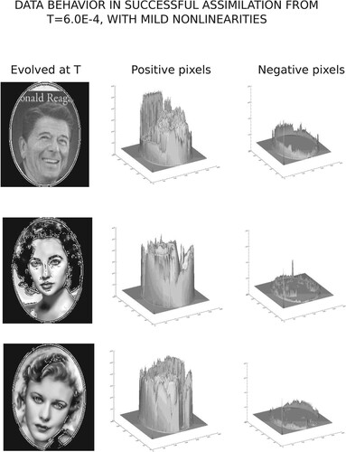
Table 2. Successful data assimilation with mild nonlinearity.

Image	Desired at $T_{max}$	Computed at 0	Evolved at $T_{max}$	${\mathcal{L}}^1$ Err
Reagan	0 $\le u\le 255$	$-153\le u\le 360$	$-29\le u\le 316$	$5\mathrm{\%}$
Taylor	$0\le v\le 255$	$-122\le v\le 395$	$-37\le v\le 285$	$6\mathrm{\%}$
Rogers	$0\le w\le 255$	$-33\le w\le 286$	$-25\le w\le 283$	$4\mathrm{\%}$

Note: Range of data values and ${\mathcal{L}}^1$ relative errors, from target at $T_{max}=6.0\times {10}^{-4}$.

Figure 3 displays the intensity data associated with the evolved data at $T_{max}$, shown in the third column of Figure 2. In the rightmost column of Figure 3, the magnitudes of the negative pixel values are shown, and compared with the significantly larger positive pixel values in the middle column of Figure 3. The results in Table 2 and Figure 3, suggest application of the following constraint to the evolved data at $T_{max}$ in the third column of Figure 2, namely, replace any pixel value exceeding 255 by the value 255, and replace any negative pixel value by the value zero. This results in the rightmost column ‘Evolved +’ in Figure 2, which is almost indistinguishable from the leftmost column in Figure 2. However, less successful results are obtained in this experiment when larger values of $T_{max}$ are used.

In the next experiment, summarized in Figures 4, 5, and Table 3, a smaller value of $T_{max}$ is used, $T_{max}=4.5\times {10}^{-4}$, but a stronger nonlinearity is considered in the system in Equation (1(1) $\begin{array}{rl}& u_t=-\text{β}Lu-\alpha Lv,\\ & v_t=Lw+\alpha Lu,\\ & w_t=-Lv,\\ & u(x,y,0)=f(x,y),v(x,y,0)=g(x,y),w(x,y,0)=h(x,y),\\ & u(x,y,t)=v(x,y,t)=w(x,y,t)=0,(x,y,t)\in \mathrm{\partial }\mathrm{\Omega }\times [0,T_{max}].\end{array}$(1) ), with $\gamma =0.05$ in Equation (26(26) $\begin{array}{rl}s\left(z\right)& =\exp \left\{0.0075\sqrt{|z]}\right\},\gamma =0.01,\\ q(x,y,t)& =\exp \left(10t\right)\{1+2\sin \pi x\sin \pi y\}\ge 1.\end{array}$(26) ). Moreover, different hypothetical data are used in the leftmost column of Figure 4, with the USAF Resolution chart replacing the Ronald Reagan stamp image, and an Alphanumeric image replacing the Ginger Rogers image. Data assimilation is highly unsuccessful in this case, with severe artifacts in the images in the second and third columns from the left in Figure 4, reflecting the very large negative and positive pixel values shown in Table 3. Now, the ${\mathcal{L}}^1$ relative errors range from $89\mathrm{\%}$ to $103\mathrm{\%}$ in Table 3. In Figure 5, the intensity data associated with the evolved data at $T_{max}$, shows equally large positive and negative pixel values. Applying the constraint $0\le z(x,y)\le 255$, is not meaningful in this case, and produces the barely recognizable rightmost column ‘Evolved +’ in Figure 4.

Figure 4. Leftmost column is the hypothetical data $W^{\ast }(\cdot ,T_{max})$. Second column from left is $U(\cdot ,0)$, the backward computation to t = 0, using the hypothetical data at $T_{max}$. Third column from left is the forward evolution at time $T_{max}$, of the computed initial data $U(\cdot ,0)$ at t = 0, shown in previous column. Last column is the result of applying the constraint $0\le z(x,y)\le 255$ to the data in the previous column.

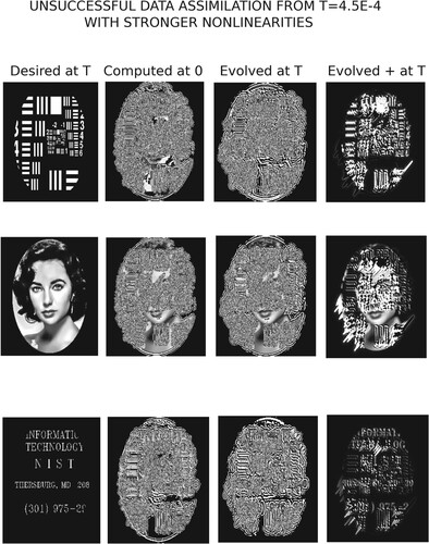
Figure 5. Magnitudes of positive and negative pixel values in ‘Evolved’ column in Figure 4. The equally large positive and negative values in this unsuccessful example are reflected in the large ${\mathcal{L}}^1$ relative errors in Table 3, and the behavior in the ‘Evolved +’ column in Figure 4.

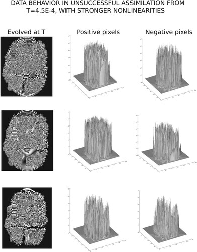
Table 3. Unsuccessful data assimilation with stronger nonlinearity.

Image	Desired at $T_{max}$	Computed at 0	Evolved at $T_{max}$	${\mathcal{L}}^1$ Err
USAF	0 $\le u\le 255$	$-6218\le u\le 6594$	$-9222\le u\le 14508$	$96\mathrm{\%}$
Taylor	$0\le v\le 255$	$-5763\le v\le 9109$	$-9889\le v\le 10963$	$89\mathrm{\%}$
Alpha	$0\le w\le 255$	$-2029\le w\le 3250$	$-4464\le w\le 7429$	$103\mathrm{\%}$

Note: Range of data values and ${\mathcal{L}}^1$ relative errors, from target at $T_{max}=4.5\times {10}^{-4}$.

6. Concluding remarks

In [16,17], and the present paper, non iterative direct methods, based on stabilized explicit backward marching finite difference schemes, were applied to 2D data assimilation problems, involving highly non smooth target data that did not correspond to actual solutions at time $T_{max}>0$. Successful and unsuccessful assimilation examples were presented. Of significant interest is whether equally good or better results can be obtained, on these or similar examples, using iterative methods such as are discussed in [1–15].

Disclosure statement

No potential conflict of interest was reported by the author(s).

References

- He Q, Barajas-Solano D, Tartakovsky G, et al. Physics-informed neural networks for multiphysics data assimilation with application to subsurface transport. Adv Water Resour. 2020;141:103610. doi: 10.1016/j.advwatres.2020.103610
- Arcucci R, Zhu J, Hu S, et al. Deep data assimilation: integrating deep learning with data assimilation. Appl Sci. 2021;11:1114. doi: 10.3390/app11031114
- Antil H, Lohner R, Price R. Data assimilation with deep neural nets informed by nudging. preprint, Nov 2021. arXiv:abs/2111.11505.
- Chen C, Dou Y, Chen J, et al. A novel neural network training framework with data assimilation. J Supercomput. 2022;78:19020–19045. doi: 10.1007/s11227-04629-7
- Lundvall J, Kozlov V, Weinerfelt P. Iterative methods for data assimilation for Burgers' equation. J Inverse Ill-Posed Probl. 2006;14:505–535. doi: 10.1515/156939406778247589
- Auroux D, Blum J. A nudging-based data assimilation method for oceanographuc problems: the back and forth nudging (BFN) algorithm. Proc Geophys. 2008;15:305–319. doi: 10.5194/npg-15-305-2008
- Ou K, Jameson A. Unsteady adjoint method for the optimal control of advection and Burgers' equation using high order spectral difference method. In: 49th AIAA Aerospace Science Meeting; 2011 Jan 4–7; Orlando, Florida.
- Auroux D, Nodet M. The back and forth nudging algorithm for data assimilation problems: theoretical results on transport equations. ESAIM:COCV. 2012;18:318–342.
- Auroux D, Bansart P, Blum J. An evolution of the back and forth nudging for geophysical data assimilation: application to Burgers equation and comparison. Inverse Probl Sci Eng. 2013;21:399–419. doi: 10.1080/17415977.2012.712528
- Allahverdi N, Pozo A, Zuazua E. Numerical aspects of large-time optimal control of Burgers' equation. Esaim Math Model Numer Anal. 2016;50:1371–1401. doi: 10.1051/m2an/2015076
- Gosse L, Zuazua E. Filtered gradient algorithms for inverse design problems of one-dimensional Burgers equation. In: Gosse L, Natalini R, editors. Innovative algorithms and analysis. Cham: Springer; 2017. p. 197–227. doi: 10.1007/978-3-319-49262-9
- de Campos Velho HF, Barbosa VCF, Cocke S. Special issue on inverse problems in geosciences. Inverse Probl Sci Eng. 2013;21:355–356. doi: 10.1080/17415977.2012.712532
- Gomez-Hernandez JJ, Xu T. Contaminant source identification in acquifers: a critical view. Math Geosci. 2022;54:437–458. doi: 10.1007/s11004-021-09976-4
- Xu T, Zhang W, Gomez-Hernandez JJ, et al. Non-point contaminant source identification in an acquifer using the ensemble smoother with multiple data assimilation. J Hydrol. 2022;606:127405. doi: 10.1016/j.jhydrol.2021.127405
- Vukicevic T, Steyskal M, Hecht M. Properties of advection algorithms in the context of variational data assimilation. Mon Weather Rev. 2001;129:1221–1231. doi: 10.1175/1520-0493(2001)129¡1221:POAAIT¿2.0.CO;2
- Carasso AS. Data assimilation in 2D viscous Burgers equation using a stabilized explicit finite difference scheme run backward in time. Inverse Probl Sci Eng. 2021;29:3475–3489. doi: 10.1080/17415977.2021.200947
- Carasso AS. Data assimilation in 2D nonlinear advection diffusion equations, using an explicit stabilized leapfrog scheme run backwrd in time. NIST Technical Note 2227, 2022 Jul 12.doi: 10.6028/NIST.TN2227
- Carasso AS. Compensating operators and stable backward in time marching in nonlinear parabolic equations. Int J Geomath. 2014;5:1–16. doi: 10.1007/s13137-014-0057-1
- Carasso AS. Stable explicit time-marching in well-posed or ill-posed nonlinear parabolic equations. Inverse Probl Sci Eng. 2016;24:1364–1384. doi: 10.1080/17415977.2015.1110150
- Carasso AS. Stable explicit marching scheme in ill-posed time-reversed viscous wave equations. Inverse Probl Sci Eng. 2016;24:1454–1474. doi: 10.1080/17415977.2015.1124429
- Carasso AS. Stabilized Richardson leapfrog scheme in explicit stepwise computation of forward or backward nonlinear parabolic equations. Inverse Probl Sci Eng. 2017;25:1–24. doi: 10.1080/17415977.2017.1281270
- Carasso AS. Stabilized backward in time explicit marching schemes in the numerical computation of ill-posed time-reversed hyperbolic/parabolic systems. Inverse Probl Sci Eng. 2018;1:1–32. doi: 10.1080/17415977.2018.1446952
- Carasso AS. Stable explicit stepwise marching scheme in ill- posed time-reversed 2D Burgers' equation. Inverse Probl Sci Eng. 2018;27(12):1–17. doi: 10.1080/17415977.2018.1523905
- Carasso AS. Computing ill-posed time-reversed 2D Navier-Stokes equations, using a stabilized explicit finite difference scheme marching backward in time. Inverse Probl Sci Eng. 2020; 28:988–1010. doi: 10.1080/17415977.2019.1698564
- Carasso AS. Stabilized leapfrog scheme run backward in time, and the explicit O(Δt)2 stepwise computation of ill-posed time-reversed 2D Navier-Stokes equations. Inverse Probl Sci Eng. 2021; 29:3062–3085. doi: 10.1080/17415977.2021.1972997
- Richtmyer RD, Morton KW. Difference methods for initial value problems. 2nd ed., New York (NY): Wiley; 1967.
- Liu Z, Renardy M. A note on the equations of a thermoelastic plate. Appl Math Lett. 1995;8:1–6. doi: 10.1016/0893-9659(95)00020-Q
- Liu K, Liu Z. Exponential stability and analyticity of abstract linear thermoelastic systems. Z Angew Math Phys. 1997;48:885–904. doi: 10.1007/s000330050071
- Liu Z, Zheng S. Semigroups associated with dissipative systems. New York: Chapman and Hall/CRC; 1999.
- Lasiecka I, Triggiani R. Analyticity, and lack thereof, of thermoelastic semigroups. ESAIM Proc. 1998;4:199–222. doi: 10.1051/proc:1998029
- Morse PM, Feshbach H. Methods of theoretical physics. New York (NY): McGraw-Hill; 1953.
- Arendt W, Ter Elst AFM. Gaussian estimates for second order elliptic operators with boundary conditions. J Oper Theory. 1997;38:87–130.
- Aronson DG. Bounds for the fundamental solution of a parabolic equation. Bull Am Math Soc. 1967;73:890–896. doi: 10.1090/bull/1967-73-06
- Ouhabaz EM. Gaussian estimates and holomorphy of semigroups. Proc Am Math Soc. 1995;123:1465–1474. doi: 10.1090/proc/1995-123-05
- Ouhabaz EM. Gaussian upper bounds for heat kernels of second order elliptic operators with complex coefficients on arbitrary domains. J Oper Theory. 2004;51:335–360.