Data Science Distance: When Close Seems Far

Abstract

Distance measures lie at the core of many data science methods. Euclidean distance can measure the distance between two points in space, Levenshtein distance can measure the difference between two words, and cosine distance can measure the angular distance between two vectors. Finding the right sense of distance is of integral importance in data science. Else, a method can produce “optimal” results under a distance measure but not match our physical and cognitive experience. In this article, we will see visually how the choice of distance in colors fundamentally impacts an algorithm. In particular, different measures result in different mosaics, including mosaics produced by colorful candies and emoji.

Keywords:

• Distance formula
• Euclidean distance
• CIELAB color model
• data science
• photomosaics

Introduction

Distance measures lie at the core of many data science methods. Euclidean distance can measure the distance between two points in space, Levenshtein distance can measure the difference between two words, and cosine distance can measure the angular distance between two vectors. Finding the right sense of distance is of integral importance in data science. Else, a method can produce “optimal” results under a distance measure but not match our physical and cognitive experience. In this article, we will see visually how the choice of distance in colors fundamentally impacts an algorithm. The authors have found this example helps contextualize more abstract choices in their work in data science.

Color is a fundamental building block for the world around us. Developers and designers choose the colors of the architecture around us, nature has developed its own colors through millions of years of evolutionary processes, and responding to our sensitivity to color, which can vary widely, we choose our own color palette through our own senses of style. We differentiate colors, consciously and subconsciously, every day.

The problem

To give context to differences in measuring the distance of colors, we’ll algorithmically create photomosaics. Specifically, a target image is partitioned into blocks, each of size $(a\times b).$ If the target image is of size $(\mathit{\text{ma}}\times \mathit{\text{nb}}),$ then the partitioning results in m rows and n columns of blocks. Else, a few options include excluding rows or columns of pixels in the target image (which is akin to cropping the image so it is $(\mathit{\text{ma}}\times \mathit{\text{nb}})$) or, in essence, expanding the image with rows or columns of background pixels (which one could choose to be a color of choice) so the expanded image’s size is $(\mathit{\text{ma}}\times \mathit{\text{nb}}).$ Then, each $(a\times b)$ 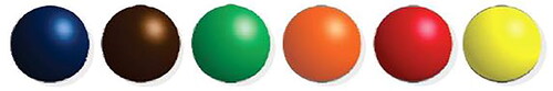block of the target image is overwritten with a new image, which we call a sub-image. The sub-image can be a single color if one were making a mosaic of Legos, for instance, or images themselves. The goal is to minimize the distance or difference between the average color of the assigned sub-image and the average color of the pixels in the block of the target image. For this paper, the target image is shown in Figure 1, and the sub-images are shown in Figure 2.

Figure 1. The target image for mosaic generation.

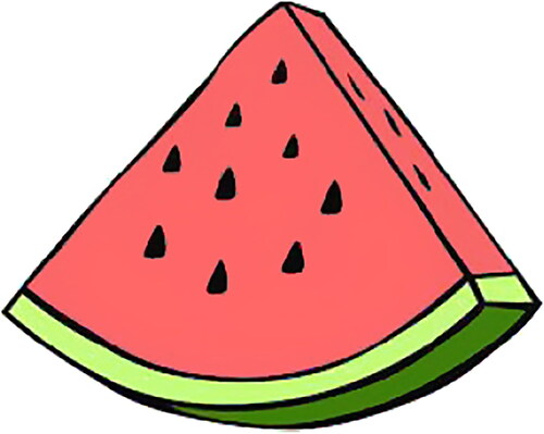
Figure 2. The six images used to create the mosaics.

We will replace each block with the sub-image that has an average color that is closest to the average color of the block. (The details of storing color and computing average color will come.) For example, the block in Figure 3a will be replaced with an image like that in Figure 3b. From the selection of options in Figure 2, is Figure 3b the best choice to replace Figure 3a? How does an algorithm determine this?

Figure 3. The linear program will attempt to minimize the color difference between each assigned sub-image (a) and each block of the target image (b).

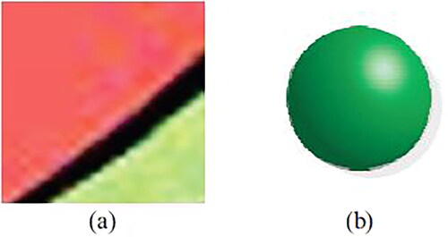
Stating this question in the context of distance, which image in Figure 2 has an overall color that is closest to the overall color in Figure 1? As such, the problem of how to quantify color differences plays a fundamental role in the resulting mosaic.

The RGB model and its issues with distance

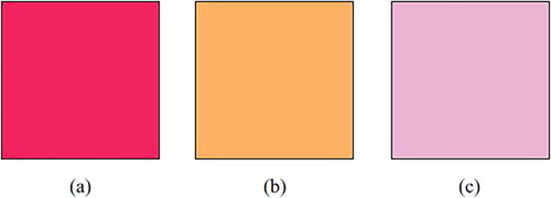
As one addresses this problem, it’s natural to turn to the most common color model in computer graphics, the RGB model, which defines a color based on the amount of red, green, and blue it contains. A pixel is stored as $(r,g,b),$ where r, g, and b are integers between 0 and 255, representing the amount of red, green, and blue, respectively, in the pixel. For example, the color of the square in Figure 4a is $(255,50,102)$ in the RGB model. The colors of the squares in Figure 4b and 4c have RGB values $(255,178,102)$ and $(255,180,255),$ respectively.

Figure 4. The colors of the squares in (a), (b), and (c) have RGB values of $(255,50,102),(255,178,102),$ and $(255,180,255),$ respectively.

This model is helpful for several reasons; first, the human eye contains three cones that are each most sensitive to different wavelengths of light. Though there is overlap between the wavelengths that the cones are sensitive to, the colors red, green, and blue are relatively closely aligned with the peak sensitivities of each of these cones. Note that this explanation is dramatically oversimplified. For more information, an interested reader can reference [1] or [2]. Second, the simple RGB model encompasses a large amount of the true color space and therefore allows for a large array of colors to be represented, as shown in Figure 5. Finally, the RGB model is an additive model in which colors are created by adding together a certain amount of red, green, and blue. This additive property makes the RGB color model useful in such areas as image display, where tiny pixels contain varying amounts of red, green, and blue light and are placed next to each other so our brains “see” different colors. (If you’ve ever pressed your eye up against an old TV screen, you may have seen those individual red, green, and blue pixels!)

Figure 5. The RGB color space compared to the entire visible spectrum [3]. Note how the RGB color triangle encompasses much of the visible spectrum.

RGB and photomosaics

Using the RGB model, a pixel in the sub-image will be stored as $(r_s,g_s,b_s),$ and a pixel in a block of the target image will be stored as $(r_t,g_t,b_t),$ where $r_s,g_s,b_s,r_t,g_t,$ and $b_t$ are integers between 0 and 255. Thus, the average color, $(R_s,G_s,B_s),$ of a sub-image is the average red, blue, and green intensities over all its pixels. Note, $R_s,G_s,$ and $B_s$ won’t necessarily be integers but still range between 0 and 255. Similarly, the average color, $(R_t,G_t,B_t),$ of a block of the target image is the average red, blue, and green intensities over all its pixels.

The distance between $(R_s,G_s,B_s)$ and $(R_t,G_t,B_t)$ can be viewed as the distance between two points in 3-space. As such, we can measure the distance between two colors stored in RGB color space as the Euclidean distance between the colors, making the distance between $(R_s,G_s,B_s)$ and $(R_t,G_t,B_t):$ $$D_{i,j}=\sqrt{{(R_s-R_t)}^2+{(G_s-G_t)}^2+{(B_s-B_t)}^2}.$$

To create our photomosaic, we find the average color for every sub-image in Figure 2. For a block in the target image, we find it’s average color and replace the block with the subimage with the closest average color as measured by the Euclidean distance.

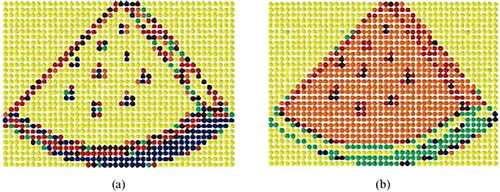
Running this model with Figure 1 as the target image and Figure 2 as the sub-images, we get the results shown in Figure 6a. The frequent use of yellow colored candies can be surprising, especially when one looks at the options for sub-images in Figure 2. A closer color match would be the red or orange sub-images. Further, the green rind of the watermelon is also visually problematic with largely blue sub-images being assigned by our algorithm to this region. How can such color choices be optimal?

Figure 6. The difference between using RGB and $\Delta E^{*}$ is striking when generating image mosaics. The mosaic generated using Euclidean distance within the RGB model is seen in (a) and the image via the $\Delta E^{*}$ within the CIELAB model is seen in (b).

To help explain our algorithm’s sense of optimality, let’s look at blocks with constant colors, as given in Figure 4. The squares in Figure 4a–c have RGB values of $(255,50,102),(255,178,102),$ and $(255,180,255),$ respectively. The distance between $(255,50,102)$ and $(255,178,102)$ is $$\sqrt{{(255-255)}^2+{(50-178)}^2+{(102-102)}^2}=128.$$

The distance between $(255,50,102)$ and $(255,180,255)$ is $$\sqrt{{(255-255)}^2+{(50-180)}^2+{(102-255)}^2}\approx \mathrm{200.8.}$$

Therefore, Euclidean distance would determine the square in Figure 4a is closer in color to the square in Figure 4b than the square in Figure 4c, although many people would likely disagree.

Is our algorithm doomed? Only if our program simply must use Euclidean distance. We chose to define an optimal solution as minimizing the Euclidean distance of the average color of an assigned sub-image and the average color of the corresponding block over the entire image within the RGB color space. We need a measure of distance that more closely matches visual differences in color.

A similar phenomenon happens in more abstract data science problems. An algorithm with a defined distance measure can lead to nonsensical results. When this happens, the data scientist needs to consider if better results could be attained with another distance measure. Or, is another overarching data science technique a better fit for the problem of interest? Let’s consider another distance measure for colors.

The CIELAB model and $\Delta E_{00}^{*}$

The CIELAB color model was developed in an attempt to address the fact that existing color models were not uniform; that is, distances between colors within the color spaces did not correspond to perceptual differences between colors as perceived by the human eye. Adopted by the International Commission on Illumination (Commission internationale de l’éclairage, or CIE) in 1974, the CIELAB color model defines a color within the $(L,a*,b*)$-space (also known as the CIELAB color space), where the L coordinate defines the color’s lightness (0 is black, 100 is white), the $a*$ coordinate defines the color’s position on the green-red axis (green is negative, red is positive), and the $b*$ coordinate defines the color’s position on the blue-yellow axis (blue is negative, yellow is positive). Despite the intent, the model is not perfectly uniform, so Euclidean distance is still not a feasible distance function to use. As such, researchers developed a color difference formula, the latest of which was developed by Luo et al. [4] and is known as $\Delta E_{00}^{*},$ to be used within the CIELAB color space. This color formula is arguably the most well-calibrated formula for numerically defining color differences as perceived by what the CIE calls the “standard observer” [5], and seems to fit well to our problem, given that perceptual color difference is exactly what we want our program to minimize.

CIELAB and photomosaics

In this case, rather than using the RGB color model and Euclidean distance to represent color differences between sub-images and blocks of the target image, the CIELAB color space is used, with the $\Delta E_{00}^{*}$ formula dictating numerical differences between colors. The $\Delta E_{00}^{*}$ is given at the end of the paper as the impact of the change in how to measure distance is the focus of this paper.

Again, color differences will be computed pixel-wise – same as with the RGB color space – over the sub-images and blocks of the target image. This time, average CIELAB color space values will be taken to determine a single value for the color of the overall block and sub-image. As such, our program analyzes the average $\Delta E_{00}^{*}$ value between pixels of the sub-image and a block of the target image.

Using the CIELAB color model has a drastic effect on the resulting mosaic, as seen in Figure 6 (b). The mosaic from the CIELAB color model, as opposed to the RGB model, is more pleasing visually. The green edge of the watermelon is evident, the black seeds in the middle have remained, and the center of the watermelon actually has a watermelon color, unlike its RGB counterpart. Coloring is not a perfect match since our solution space is limited by the sub-images shown in Figure 2. Including more colors within the sub-images would certaintly lead to an even better approximation of the target image.

Distant conclusions

This simple experiment highlights the importance of considering the impact of the metrics underlying an experiment at hand. In this case, the consequences are apparent but not preventative; however, in other cases, the consequences of using a metric that is not well-suited to the problem could be more costly.

Though it gives better results than Euclidean distance in the RGB color space, as desired, the CIELAB color difference formula makes our program more computationally intensive. The difference is imperceivable when a mosaic is constructed using the small set of images in Figure 2. This changes when the number of images available in a mosaic grows. There may be less computationally costly metrics that could acheive results quite close to the CIELAB color model, especially given our results are mosaic approximations.

Further, the $\Delta E_{00}^{*}$ formula, given in the next section, is neither simple nor quickly digestable. At times, simplicity is helpful in data science, even when overall accuracy is reduced. This is inherent in modeling. Simplifying assumptions can be removed. In a way, moving from the RGB color space to the CIELAB color space is an increase in complexity.

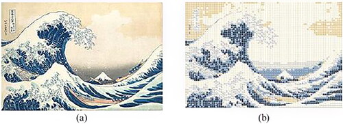
Note, such mosaics can have considerable detail. In Figure 7, we see an approximation of “The Great Wave off Kanagawa” by Katsushika Hokusai (1831) seen in (a) using sub-images that are emojis. With enough patience, you could tap out the sequence of emojis on our phone or computer to create the approximation in (b).

Figure 7. Using “The Great Wave off Kanagawa” by Katsushika Hokusai (1831) as a target image (a) can produce the mosaic in (b) created entirely with emojis using the CIELAB color space.

To find the distance between two colors in CIELAB color space, $(L_1^{*},a_1^{*},b_1^{*}),$ and $(L_2^{*},a_2^{*},b_2^{*})$ equals: $$\Delta E_{00}^{*}=\sqrt{{\left(\frac{\Delta L^{\prime }}{k_L{S}_k}\right)}^2+{\left(\frac{\Delta C^{\prime }}{k_C{S}_C}\right)}^2+{\left(\frac{\Delta H^{\prime }}{k_H{S}_H}\right)}^2+R_T\frac{\Delta C^{\prime }}{k_C{S}_C}\frac{\Delta H^{\prime }}{k_H{S}_H}},$$

where $$\begin{array}{c}\Delta L^{\prime }=L_2^{*}-L_1^{*},\hfill \\ \overline{L}=\frac{L_1^{*}+L_2^{*}}{2},\overline{C}=\frac{C_1^{*}+C_2^{*}}{2},\hfill \\ a_1^{\prime }=a_1^{*}+\frac{a_1^{*}}{2}\left(1-\sqrt{\frac{{\overline{C}}^7}{{\overline{C}}^7+{25}^7}}\right),\hfill \\ a_2^{\prime }=a_2^{*}+\frac{a_2^{*}}{2}\left(1-\sqrt{\frac{{\overline{C}}^7}{{\overline{C}}^7+{25}^7}}\right)\hfill \\ {\overline{C}}^{\prime }=\frac{C_1^{\prime }+C_2^{\prime }}{2}\text{and}\Delta C^{\prime }=C_2^{\prime }-C_1^{\prime }\hfill \\ \text{where}{C}_1^{\prime }=\sqrt{a_1^{{}^{\prime }2}+b_1^{*2}},C_2^{\prime }=\sqrt{a_2^{{}^{\prime }2}+b_2^{*2}}\hfill \\ h_1^{\prime }=\mathrm{\text{atan}}2(b_1^{*},a_1^{\prime })\hspace{1em}\mathrm{\text{mod }}{360}^{°},h_2^{\prime }=\mathrm{\text{atan}}2(b_2^{*},a_2^{\prime })\hspace{1em}\hfill \\ \mathrm{\text{mod }}{360}^{°}\hfill \end{array}$$ $$\begin{array}{l}\Delta h^{\prime }=\{\begin{array}{cc}{h}_2^{\prime }-h_1^{\prime }\hfill & |h_1^{\prime }-h_2^{\prime }|\le {180}^{°}\hfill \\ h_2^{\prime }-h_1^{\prime }+{360}^{°}\hfill & |h_1^{\prime }-h_2^{\prime }|>{180}^{°},h_2^{\prime }\le h_1^{\prime }\hfill \\ h_2^{\prime }-h_1^{\prime }-{360}^{°}\hfill & |h_1^{\prime }-h_2^{\prime }|>{180}^{°},h_2^{\prime }>h_1^{\prime }\hfill \end{array}\hfill \\ \Delta H^{\prime }=2\sqrt{C_1^{\prime }{C}_2^{\prime }}\hspace{0.17em}\mathrm{\text{sin}}\hspace{0.17em}(\Delta h^{\prime }/2),{\overline{H}}^{\prime }=\{\begin{array}{cc}(h_1^{\prime }+h_2^{\prime })/2\hfill & |h_1^{\prime }-h_2^{\prime }|\le {180}^{°}\hfill \\ (h_1^{\prime }+h_2^{\prime }+{360}^{°})/2\hfill & |h_1^{\prime }-h_2^{\prime }|>{180}^{°},h_2^{\prime }+h_1^{\prime }<{360}^{°}\hfill \\ (h_1^{\prime }+h_2^{\prime }-{360}^{°})/2\hfill & |h_1^{\prime }-h_2^{\prime }|>{180}^{°},h_2^{\prime }+h_1^{\prime }\ge {360}^{°}\hfill \end{array}\hfill \\ T=1-0.17\hspace{0.17em}\mathrm{\text{cos}}\hspace{0.17em}({\overline{H}}^{\prime }-{30}^{°})+0.24\hspace{0.17em}\mathrm{\text{cos}}\hspace{0.17em}(2{\overline{H}}^{\prime })+0.32\hspace{0.17em}\mathrm{\text{cos}}\hspace{0.17em}(3{\overline{H}}^{\prime }+6^{°})-0.20\hspace{0.17em}\mathrm{\text{cos}}\hspace{0.17em}(4{\overline{H}}^{\prime }-{63}^{°})\hfill \\ S_L=1+\frac{0.015{(\overline{L}-50)}^2}{\sqrt{20+{(\overline{L}-50)}^2}},S_C=1+0.045{\overline{C}}^{\prime },S_H=1+0.015{\overline{C}}^{\prime }T\hfill \\ R_T=-2\sqrt{\frac{{\overline{C}}^{\prime 7}}{{\overline{C}}^{\prime 7}+{25}^7}}\hspace{0.17em}\mathrm{\text{sin}}\hspace{0.17em}\left({60}^{°}·\hspace{0.17em}\mathrm{\text{exp}}\hspace{0.17em}\left(-{\left(\frac{{\overline{H}}^{\prime }-{275}^{°}}{{25}^{°}}\right)}^2\right)\right).\hfill \end{array}$$

Disclosure statement

No potential conflict of interest was reported by the author(s).

References

- Rod Nave. The Color-Sensitive Cones. GSU HyperPhysics. 2022. http://hyperphysics.phy-astr.gsu.edu/hbase/vision/colcon.html
- Purves D, et al. Cones and color vision. In: Neuroscience. 2nd ed. Sunderland: Sinauer Associates; 2001. https://www.ncbi.nlm.nih.gov/books/NBK11059/
- Amara M, et al. Temperature and color management of silicon solar cells for building integrated photovoltaic. EPJ Photovolt. 2018;9:1. https://www.epj- doi: 10.1051/epjpv/2017008
- Luo MR, Cui G, Rigg B. The development of the CIE 2000 colour-difference formula: CIEDE2000. Color Res Appl J. 2001;26(5):340–350. doi: 10.1002/col.1049
- Schanda J. Colorimetry: Understanding the CIE system. Hoboken: John Wiley & Sons; 2007. p. 501.