Effect of image resolution on intensity based scene illumination classification using neural network

Abstract

In this paper, a framework for testing scene illumination classification with different image resolutions is proposed. The testing aims to provide the researchers with valuable information about the effect of image resolution on scene illumination classification using a neural network. The experiment is done by extracting three types of features from the images. These three types consist of statistical features, physic based features and histogram based features. It has been demonstrated that scene illumination classification can be affected by changing the image resolution. Despite the popular belief that high resolution images lead to better results, scene illumination classification by the proposed method performed best using low resolution images. At the second part of discussion, the reason behind this phenomenon is mathematically analysed and explained.

Keywords:

• Scene illumination classification
• Image resolution
• Neural network

Introduction

Recently, the amount of studies on image classification has increased significantly due to its wide usage in many different applications, especially scene illumination classification, which focuses on classifying the properties of light in the scene to prepare them for further applications like correction.

Scene illumination classification can be helpful in object recognition and detection, white balance, color constancy, color reproduction, illumination correction, intelligent vehicle and robot navigation.^1,2

The huge progress in imaging systems enables users to capture images with very high resolution, such as 15 to 20 megapixels, even for compact cameras for home entertainment. Although super high resolution cameras that are able to take photos with resolutions up to a couple of gigapixels are on the way to the market, these high resolution images bring various side effects for applications that want to use them. For instance, transferring, storing, retrieving, querying and processing will be more costly. In addition, many applications are not able to process high resolution images due to their limitations. The hypothesis that “a higher resolution will to better performance” is widespread.

The question of “Do high resolution images deliver better performance?” is a general question that can be modified to any image processing system or method and has been previously explored by various studies to answer the aforementioned concern. The motivation behind this study is to answer the above question in scene illumination classification field and to propose the optimum resolution. Finding this optimised resolution has some major achievements. First, delivering better performance and accuracy. Second, reduce the processing load by avoiding processing the unnecessary high resolution images and subsequently decrease the response time of the system.

The relationship of image resolution and performance of face recognition has been the subject of many studies.^3–5 In summary, the findings of such research demonstrate that the performance of the face recognition system will remain constant by reducing the image resolution; however, this trend will only continue up to a certain threshold by decreasing the resolution, after which the performance will deteriorate.⁶ In Ref. 3, the authors investigated the effect of image resolution on the performance of a face recognition system. This experiment is done in three parts: face detection, face registration and normalisation and face recognition. The experiment is repeated for the same images but various resolution starting from 128 × 128 to 8 × 8 and each time tested on separate face components. Their results proved that the face recognition system is not very sensitive to image resolution, and moreover, good accuracy can still be obtained by reducing the image resolution to 32 × 32 pixels. In a separate study,⁷ the authors try to know “Are high resolution images are more effective in face recognition results?” The results achieved by this study also demonstrate that relatively low resolution images perform better than high resolution representation. In this study, a neural network is applied to accomplish the recognition with the basic assumption of “high resolution images the amounts of noise contaminated pixels are higher.”

Nevertheless, low resolution images have been acknowledged to be suitable for certain applications. However, decreasing the image resolution increases the effect of noise, which means these tiny images are not appropriate for some general purposes.⁸ The experiment done in Ref. 8 shows that full resolution images delivered better accuracy compared to resized images in terms of non-parametric object recognition. This can be related to the types of feature applied in the experiment.

In the multimedia field, this issue has been addressed by various studies that focused on object or movement recognition. For example, in order to boost the accuracy of detecting a full 3D body scan, the approach of using high resolution images was proposed.⁹ However, this approach was later implemented by combining several low resolution images from multiple views.¹⁰ Such a method not only benefits from low resolution images but also obtained more accurate representation compared to its predecessors.

In medical imaging, one study focused on surveying the effect of the image resolution on the accuracy of its system. The final presented results showed that a higher image resolution leads to better accuracy, albeit there is some limitation in increasing the image resolution due to the increased amount of noise.¹¹

Methodology

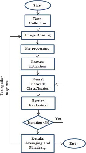
The methodology that is used for this study is a neural network based classification consisting of seven main steps. The steps are shown in Fig. 1.

1 Step by step flow chart of implemented system

A database of 338 scene images was applied in this study with resolution of 4368 × 2096. Then, the images are presented with six different image resolutions: 2048 × 2048, 1024 × 1024, 512 × 512, 256 × 256, 128 × 128 and 64 × 64. For each image set with specific resolution, the corresponding feature set has been extracted. The process of resizing the images is done by using the following two steps: first dividing the image to equal size windows and then merging the pixel values of each window into one single pixel. The intensity of such pixel is the average intensity of all exciting pixels in the window⁷ (Fig. 1, image resizing).

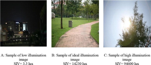
All original images are accompanied by the surrounding illumination value (SIV).¹² The SIV as a physics based feature presents the amount of light at the moment of capturing the photo (Fig. 1, feature extraction). Using SIV can help bridge the gap between the image presented data and the real data from the scene (Fig. 2).

2 Sample of input images with their corresponding SIV value

The second class of input feature was a subset of statistical scene illumination classification approaches.^13,14 The statistical feature set consists of mean, mode and median of the image illumination, which were all extracted from the Y component of the image and transferred from the RGB color model to CIE XYZ.

The range of varying illumination (0 to 117000 lux) in the real scene was mapped from 0 to 255 in the image illumination component (Y). Therefore, a direct relationship between the real scene illumination and the image illumination could be deduced. The mean of illumination depicts the average illumination of the image pixels, which is equivalent to SIV and represents the illumination of the real scene. The mode of illumination can help in determining the most frequent illumination value that could be helpful in finding light spots. The median of image illumination represents the varying range of illumination in the image.

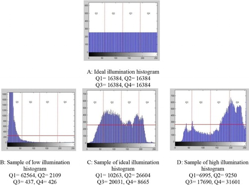
The third type of input feature for this classification system was the histogram quartering feature. This feature helps to increase the performance of classification by better histogram comparison. The illumination histogram of the image was divided into four quarters and then compared to the corresponding quarter of the most ideal image illumination histogram (Fig. 3). The differences are presented in four values for the four histogram quarters.

3 Sample of image histograms (256 × 256) with their corresponding quarter's value. Vertical lines separating quarters from each other and horizontal line refer to ideal histogram level. Horizontal axis represents CIE XYZ y component value; vertical axis represents number of pixels in each Y component value

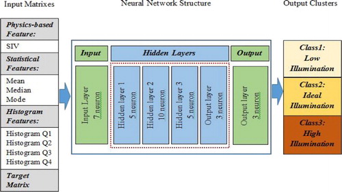
The proposed classifier for this study is a feed forward pattern recognition network with three hidden layers (Fig. 1, neural network classification). The number of neurons in the layers are 5, 10 and 5 for the first, second and third layers respectively. All the aforementioned extracted features are the inputs of this network. Using a target matrix that indicates the belonging group of the training samples enables the network to sort out the test samples into predefined clusters (Fig. 4). Levenberg–Marquardt is used as a training algorithm for this network, which is highly recommended as a first choice supervised algorithm for those problems that have up to a few hundreds of weight.¹⁵

4 Designed neural network structure: eight inputs correspond to eight features (mean, mode, median, SIV and Q1 to Q4), and three outputs correspond to three output clusters (low, ideal and high illumination)

Starting from the highest image resolution set (2048 × 2048), the corresponding feature set was the input of the neural network. In addition, a target matrix carrying the belonging group of each image was also fed into the neural network for the training phase. Then, the process of classification was repeated 30 times to guarantee the accuracy of the system.

The training algorithm performance was monitored by mean square error (MSE) (Fig. 1, result evaluation); this parameter was used as one of the evaluating and comparing parameters of the system.^16,17 In order to have a very clear understandable estimate of the system performance, the error percentage was proposed. The classification error or simply the misclassification rate is the ultimate measure of the performance of a classifier. The capability of defining a target value based on reducing the misclassification rate is another motivating point for using it.¹⁸ Since any estimation may follow a prediction, providing an accurate measure for system prediction, efficiency is necessary. Using the coefficient of determination (R square) as the measure of system accuracy in order to compare the estimated value and the proposed model is a common solution for evaluating the system efficiency in this aspect.¹⁹

Finally, for each image resolution set, the classification process was done, and the results recorded in terms of accuracy rate, MSE and R square value (Fig. 1, iteration and result finalising). All the recorded values are the average of 30 times repeat of the test. The 30 times repeat will minimise the inherent randomness behavior in the training procedure of the neural network.¹⁸ Repeating the test for 30 times will ensure the results are following a normal distribution pattern and not a random one.

Results and discussion

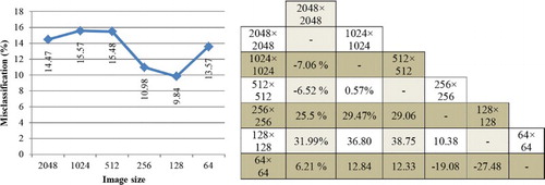
The results presented in Fig. 5 depict that the misclassification rate of the system varies by changing the image resolution. A reduction of 4.62% occurs between the lowest and highest misclassification rate, travelling from the lowest image resolution to the highest image resolution. This simply demonstrates the effect of image resolution on misclassification rate. The system misclassification rate has a downward trend by decreasing the image resolution from 2048 × 2048 to 128 × 128. This trend dramatically increases from 512 × 512 to 128 × 128. Then, after that, by reducing the image resolution, the upward trend starts. As an example on how to use the table in Fig. 5, let us assume that there is an image with resolution of 1024 × 1024; then, by referring to the table, we can see that if the resolution decreased to 512 × 512 the misclassification rate will improve by 0.57%, if reduced to the misclassification rate will improve by 29.47% and finally reducing the image resolution to 128 ×  128 will improve the rate by 31.99%.

5 Misclassification rate analysis. On left, chart shows misclassification rate changes by changing image resolution. On right, separated improvement of each image resolution is compared to others by percentages. Negative values in table show that instead of reduction increase occurred

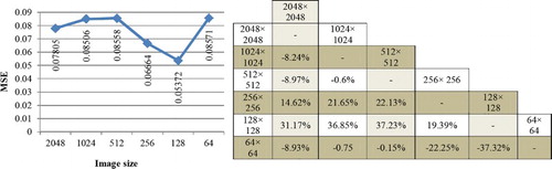
The same scenario happens in the MSE chart. Figure 6 clearly depicts the effect of image resolution on MSE. The general trend of the MSE chart is the same as the misclassification rate, and an improvement of 37.23% is achieved from the worst to the best case. In the MSE chart, the differences are clearer, for instance, from 256 to 128, a reduction of 1.14% occurs, whereas in the MSE, a reduction of 19.34% occurs. However, although the 1.14% is not very remarkable for some applications, the 19.34% reduction in MSE for same cases demonstrates the significant improvement delivered by reducing the image resolution from 256 to 128.

6 Mean square error analysis. On left, chart shows MSE changes by changing image resolution. On right, separated improvement of each image resolution is compared to others by percentages in terms of MSE

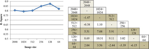
R square as a measure for goodness of fit of the modeling can represent the performance of the system for predicting based on current modeling.^19,20 As can be seen in Fig. 7, the predicting power of a scene illumination classification system is also affected by changing the image resolution. A slight continuous improvement is achieved by discounting the image resolution from 2048 to128. However, similar to the other two parameters, the trend starts to decline by reducing the image size to 64. A growth of 10.31% occurred in the R square value from the worst case up to the optimal point (128 × 128).

7 R square analysis. On left, chart shows R square changes by changing image resolution. On right, separated improvement of each image resolution is compared to others by percentages in terms of R square

The previous discussions clearly prove that decreasing the resolution up to a certain threshold will increase the performance, whereas the performance will deteriorate when the threshold is crossed. The tables in Figs. 5, 6 and 7 help to show how much improvement will be achieved in percentage by reducing the higher image resolution. To study and determine what is the reason for such behavior, we need to go back to feature sets and their corresponding values for each image resolution test. Table 1 shows the feature values for all image resolutions. For a more detailed analysis, the table presents the values for three samples, each belonging to a different illumination class.

Table 1 Feature values for three different images from various illumination classes presented by various image resolutions

Sample	Resolution	Avg	Mode	Median	Q1	Q2	Q3	Q4	CV
Low	64	54	22	53	2727	1208	132	29	1.0608
	128	54	23	52	10986	4637	601	160	1.0605
	256	54	21	51	43,858	18,334	2,503	831	1.054
	512	54	23	50	174,465	74,096	9,506	4,077	1.047
	1024	54	23	50	694,001	299,930	36,403	18,242	1.041
	2048	54	15	49	2,768,017	1,206,272	141,736	78,279	1.038
Ideal	64	109	34	104	1021	1460	1381	234	0.473
	128	109	47	103	5633	5314	1197	2660	0.427
	256	109	157	101	17,489	22,080	20,464	5503	0.397
	512	109	160	100	71,570	86,389	80,112	23,893	0.375
	1024	109	86	100	292,092	341,148	315,081	100,255	0.362
	2048	109	163	99	1,178,477	1,356,504	124,932	409891	0.356
High	64	158	248	167	640	466	1561	1429	0.1587
	128	159	248	170	2707	1691	5844	57600	0.1472
	256	159	238	171	11156	6308	24022	24050	0.1447
	512	159	255	173	46043	24512	93283	98306	0.1410
	1024	159	255	175	188512	100383	353208	406473	0.1393
	2048	159	255	175	188512	100383	353208	406473	0.1399

As can be seen in Table 1, the average illumination value remains constant by changing the image resolution. Since the resizing process is done by dividing pixels in windows and averaging them, there would be no difference in the average values in various image sizes. Hence, the average illumination value does not involve performance improvement. In the case of the median illumination value, the changes occurred in the vicinity of a certain value with very little variation. Therefore, even though the small contribution of median value in the improvement of system performance is negligible, the values for mode feature are highly affected by changing the image resolution, especially in the ideal illumination samples. For the other two groups based on the exaggerated property of light intensity, the changes in mode value are not as much as for the ideal class.

In order to analyse the effect of the image resolution changes on histogram quartering features, we need to apply the coefficient of variation (CV), which shows a normalised measure for the distribution of pixel values over four quarters. This statistic enables the changes in the quarter value of the illumination histogram to be clearly monitored by image resolution. Figure 8 depicts the effect of the image resolution changes on the CV of the histogram quarter features.

8 Coefficient of variation of histogram quarter features separated by image illumination class: (A) low illumination class, (B) ideal illumination class and (C) high illumination class

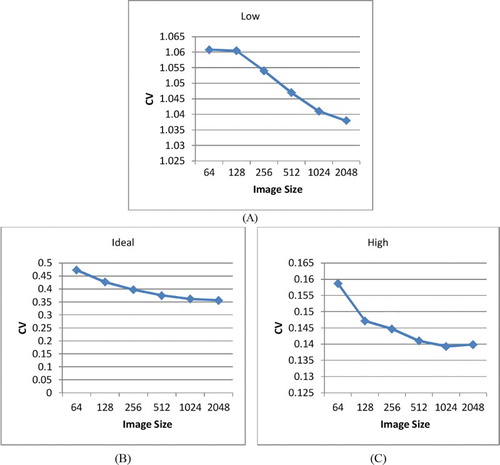
The CV for the quarters declines by increasing the image resolution. This means that the differences in quarter values are decreasing by increasing the image resolution, and the values are going to be same. This phenomenon results in reducing the discriminating power of the histogram quartering features by the neural network. Therefore, having quarter values with a higher CV (much more differences in distribution) is the main reason for having better performance for the lower resolutions.

By looking at Fig. 8 again, it can be seen that the CV for the high and low illumination samples is more affected by the image resolution than the ideal illumination. This is related to the natural histogram shape of the illumination value in each cluster. The ideal illumination histogram has closer values in each quarter, and by changing the image resolution, it has been less affected. However, the high and low illumination histograms have huge differences in the quarters, and by changing image size, they have been more influenced. Hence, the CV value in the high and low illumination samples decreased the misclassification and the error dramatically and much more than for the ideal illumination. In general, it can be concluded that changing the image resolution has much more effect on the classification of high and low illumination samples than the samples with ideal illumination.

Conclusion

The effect of image resolution on the illumination classification was investigated. The experiment shows that the performance was improved by reducing the image resolution, but this improvement only continued up to a threshold. The best performance was delivered by the image set with a resolution of 128 × 128 by improvement of 4.62% in misclassification rate, 31.17% in MSE and 8.69% in R square. As the performance started to deteriorate by reducing the image resolution to values of less than 128 × 128, this resolution setting could be set as the threshold for image illumination classification and estimation.

The changes in CV for the quarter values of the illumination histogram are acknowledged to be the main reason for performance changes. Increasing the image resolution will lead to a decrease in the CV of the histogram quarter values. Once the CV in histogram quarter values decrease, these values get more similar, and it will lead to reduction in discrimination power of NN. Finally, it will result in more misclassification, more error and lower R square value. This phenomenon affects the high and low illumination cluster more than the ideal illumination class due to the larger changes in CV in the corresponding group.

References

- Zhou, L., Zhou, Z. and Hu, D. Scene classification using a multi-resolution bag-of-features model. Pattern Recognition, 2013, 46, 424–433. doi: 10.1016/j.patcog.2012.07.017
- Tominaga, S., Ebisui, S. and Wandell A, B. Scene illuminant classification: brighter is better. JOSA A, 2001, 18, 55–64. doi: 10.1364/JOSAA.18.000055
- Boom, B., Beumer, G., Spreeuwers, L. J. and Veldhuis, R. N. The effect of image resolution on the performance of a face recognition system. 2006.
- Wang, J., Zhang, C. and Shum, H. -Y. Face image resolution versus face recognition performance based on two global methods., in Proc. Asian Conf. on 'Computer vision, Jeju Island, Korea 2004.
- Lemieux, A. and Parizeau, M. Experiments on eigenfaces robustness. Proc. 16th Int. Conf. on 'Pattern recognition, 2002, pp. 421–424.
- Fookes, C., Lin, F., Chandran, V. and Sridharan, S. Evaluation of image resolution and super-resolution on face recognition performance. J. Visual Commun. Image Represent, 2012, 23, 75–93. doi: 10.1016/j.jvcir.2011.06.004
- Chen, L., Tokuda, N., Nagai, A. and Chen, X. Is high resolution representation more effective for content based image classification?, Proc. Int. Joint Conf. on 'Neural networks, IJCNN'06 2006, pp. 4045–4050..
- Deng, J., Dong, W., Socher, R., Li, L. -J., Li, K. and Fei-Fei, L. Imagenet: a large-scale hierarchical image database., Proc. IEEE Conf. on 'Computer vision and pattern recognition, CVPR 2009, pp. 248–255..
- Anguelov, D., Srinivasan, P., Koller, D., Thrun, S., Rodgers, J. and Davis, J. Scape: shape completion and animation of people. ACM Trans. Graphics, 2005, 408–416. doi: 10.1145/1073204.1073207
- Tong, J., Zhou, J., Liu, L., Pan, Z. and Yan, H. Scanning 3d full human bodies using kinects. IEEE Trans. Visual. Comput. Graphics, 2012, 18, 643–650. doi: 10.1109/TVCG.2012.56
- Boellaard, R., Krak, N. C., Hoekstra, O. S. and Lammertsma, A. A. Effects of noise, image resolution, and ROI definition on the accuracy of standard uptake values: a simulation study. J. Nucl. Med., 2004, 45, 1519–1527.
- Hesamian, M., Mashohor, S., Saripan, M. I. and Wan Adnan, W. Scene illumination classification using illumination histogram analysis and neural network., Proc. IEEE Int. Conf. on 'Control system, computing and engineering (ICCSCE) 2013..
- Barnard, K., Cardei, V. and Funt, B. A comparison of computational color constancy algorithms. I: Methodology and experiments with synthesized data. IEEE Trans. Image Process, 2002, 11, 972–984. doi: 10.1109/TIP.2002.802531
- Ebner, M. Color constancy, 2007 (John Wiley & Sons, New York), Vol. 6.
- Hagan, M. T. and Menhaj, M. B. Training feedforward networks with the Marquardt algorithm. IEEE Trans. Neural Networks, 1994, 5, 989–993. doi: 10.1109/72.329697
- Pradeep, J., Srinivasan, E. and Himavathi, S. Diagonal based feature extraction for handwritten alphabets recognition system using neural network, arXiv preprint arXiv. 2011, 11030365.
- Weintraub, M., Beaufays, F., Rivlin, Z. e., Konig, Y. and Stolcke, A. Neural-network based measures of confidence for word recognition., Proc. IEEE Int. Conf. on 'Acoustics, speech, and signal processing 1997, 887–887..
- Devijver, P. A. and Kittler, J. Pattern recognition: a statistical approach., 1982 (Prentice-Hall, London), Vol. 761.
- Shahsavari, S., Bagheri, G., Mahjub, R., Bagheri, R., Radmehr, M., Rafiee-Tehrani, M., et al. Application of artificial neural networks for optimization of preparation of insulin nanoparticles composed of quaternized aromatic derivatives of chitosan. Drug Res., 2014, 64, 151–158.
- Armstrong, J. S. Illusions in regression analysis., 2011.