Simultaneous optimisation of structural topology and material grading using level set method

Abstract

The present paper introduces a new technique for simultaneously optimising the topology and continuous material distribution of a structure. Topology optimisation offers great potential for novel, improved structural designs and is an ideal design tool for additive manufacturing (AM) techniques. Level set based topology optimisation produces solutions with clear, smooth boundaries that can be directly fabricated using AM. Further benefits of AM may be realised by also optimising the material distribution within the structure. The sequential linear programming level set method is used to include material distribution design variables in the topology optimisation problem. This allows the topology and continuous material distribution to be optimised simultaneously. Several compliance minimisation problems are used to demonstrate the proposed approach.

Keywords:

• Design for additive manufacture
• Topology optimisation
• Level set method
• Graded material

Introduction

Modern additive manufacturing (AM) techniques can make designs with highly complex geometries and removes many conventional manufacturing constraints.^1–4 During the design process, the addition of manufacturing constraints usually results in a reduction of the design space, potentially leading to designs with lower performance compared with an unconstrained design.⁵ Thus, the expanded design space offered by AM opens up new possibilities for optimised designs.

The rapid increase in computer performance in recent decades has seen the rise in many powerful computational tools that aid engineers in achieving better, more efficient designs. This is particularly evident when advanced computational analysis tools are combined with powerful optimisation methods. Structural design is an area that has benefitted from this paradigm, where the finite element (FE) method is combined with a variety of optimisation techniques.⁶ Structural optimisation methods can be classified into three categories,⁷ as shown in Fig. 1. Sizing optimisation is usually performed on a mature structure, where the main layout and geometry have already been decided. Shape optimisation allows more freedom, as only the general layout is usually predetermined and the exact position and size of features are to be optimised. Topology optimisation methods allow the greatest freedom, as they usually make no assumptions on the layout, shape or sizing of the structure, which are all subject to optimisation. The complexity and computational cost of structural optimisation methods generally increases as the design space increases from sizing optimisation, with 10s or 100s of design variables, to topology optimisation, with 1000s of variables, or more.

1. a sizing; b shape; c topology optimisation

Categories of structural optimisation

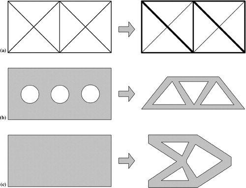
Additive manufacturing offers greater freedom to a designer and can make parts with complex geometry. Topology optimisation explores the largest design space, and the resulting geometries are often complex. Thus, there is a synergy between AM and topology optimisation that offers a new paradigm for the design and manufacture of efficient structural components.^1–4 Furthermore, the realisation of topology optimisation designs using conventional manufacturing methods requires additional constraints^8–11 or post-processing,^12,13 which adds complexity and time into the design process. Thus, the freedom enabled by AM can result in a simpler and quicker design process. Examples of the direct realisation of complex topological optimum designs via AM include bone implant scaffolds manufactured by selective laser melting,¹⁴ multimaterial compliant mechanisms made using PolyJet three-dimensional (3D) printing,¹⁵ microstructures with extreme properties^16,17 and lightweight aerospace components.^2,18

Topology optimisation is often defined as a discrete problem, where the goal is to decide at each point in the design domain whether material should be present or not. If the design space is discretised using FEs, the topology optimisation problem is then to decide if each element should contain material or not.⁷ Approaches based on this idea are sometimes called element based methods. In practice, the discrete problem is difficult to solve, so it is often relaxed such that the amount of material present in each element can range continuously from 0 (void) to 1 (solid).^19,20 To approximate the true discrete problem, the material properties of elements with an intermediate amount of material are often penalised to encourage elements to become either completely solid or completely void. In the popular solid isotropic material with penalisation (SIMP) approach to topology optimisation, a power law penalisation is used. However, other penalisation schemes can also be used, and methods based on homogenisation of microstructures have also been developed.²⁰ There are also element based methods that do not use penalisation and work directly with the 0–1 discrete problem formulation. Bidirectional evolutionary structural optimisation uses heuristic criteria to progressively remove or add material from the design by changing elements from solid to void, or void to solid respectively.²¹

Element based methods often required further techniques to avoid numerical issues such as the formation of checkerboard patterns and mesh dependent solutions.²² Element based methods have been successful in solving a wide range of engineering topology optimisation problems. However, solutions obtained with penalisation methods often contain unclear ‘fuzzy’ boundaries that require some form of post-processing to produce designs that can be manufactured, even by AM techniques.^12,13 Bidirectional evolutionary structural optimisation results also require post-processing, as they often possess jagged boundaries due to the discrete 0–1 formulation.²³ Post-processing procedures are not straightforward and do not ensure that the optimality of the structure is preserved.

To overcome the issues with element based methods and produce clear, smooth boundary solutions, boundary based topology optimisation methods have been developed. Early attempts focused on extending spline based shape optimisation methods to include hole insertion.^24,25 However, these approaches are often complex and require many specific techniques to handle topological changes, such as hole insertion or merging, and to ensure that an accurate description of the boundary is maintained during optimisation.²⁶ Interest has grown over the last 15 years in topology optimisation using implicit functions and level set methods. The key idea of the level set approach is that the structural boundary is described by an implicit function discretised at points in the design domain. If the implicit function at a point is positive, then that point is inside the structure; a negative value indicates that the point is outside the structure; and a zero value means that the point is on the boundary of the structure. Therefore, the boundary is defined as the zero level set of an implicit scalar function. The implicit boundary description naturally handles topological changes, and solutions have clear, smooth boundaries. There are several forms of level set based topology optimisation, and the interested reader is referred to some recent review papers for further details.^27–29 In the context of AM, level set based methods offer the potential to directly build an optimised design with no post-processing, which preserves the optimality of the solution and reduces the complexity and time of the design process compared with element based methods.

A further benefit of some AM techniques is the ability to build single components from more than one material.² This idea has been applied to many areas of design, including compliant mechanism that use a mixture of stiff and flexible material,^15,30,31 composite microstructures with tuned elastic and thermal properties^32–34 and stiff structures.^35,36 Topology optimisation methods have been extended to take advantage of multimaterial manufacturing techniques by including material choice as part of the design space. This approach allows the optimiser to choose not only whether material should be present at a point but also what material it should be. This expansion of the design space can produce more efficient designs compared with uniform material solutions. Most methods developed for combined topology and material optimisation treat material choice as a discrete problem and obtain solutions where each point is part of a distinct material phase. The SIMP method has been extended for two material optimisation using two variables per element.³² One variable determines if the element contains material, and the other determines the material type. To obtain distinct material phases, the material type design variable can be penalised using a power law,³³ or a material model based on the Hashin–Shtrikman bounds can be used.³⁷ Another interesting approach is projection topology optimisation, which can project discrete phases of materials onto the design space allowing for combined material and topology optimisation.^15,38 Approaches for material phase optimisation have also been developed for level set based methods using multiple level set functions³⁶ or a modified Cahn–Hilliard phase field model.³⁵

Advances in AM processes are enabling an alternative to the material phase design approach, where material can be continuously graded from one phase to another, a so-called functionally graded material (FGM). Metallic FGM structures have been produced using electron beam freeform fabrication,³⁹ where multiple feedstock wires are used to create the grading. Laser powder deposition can also create graded metals by varying the feedrate of two powered materials.⁴⁰ The PolyJet 3D AM method can create structures made from two different photopolymer materials,¹⁵ which can be combined to create materials with properties ranging between the two extremes. These fabrication processes can achieve a continuous grading of material properties, such as elastic modulus, tensile strength and hardness.

There is little work optimising the material distribution for a metallic FGM. Paulino et al.³⁴ optimised the material distribution in a microstructure to obtain extreme properties, such as a zero shear modulus or negative Poisson's ratio. Dunning et al.⁴¹ explored the use of FGM for aeroelastic tailoring using a genetic algorithm. The original extension of SIMP for two materials did not penalise the material type design variables, allowing for simultaneous optimisation of topology and the continuous distribution of two materials.³² However, to the author's knowledge, there are no other examples where topology and continuous material distribution are optimised simultaneously.

The novel contribution of the present paper is to introduce a method for simultaneously optimising the topology and material distribution of a structure using a level set method to take full advantage of advanced multimaterial AM techniques. The sequential linear programming (SLP) level set method,⁴² previously developed by the authors, is extended to include material distribution optimisation. The SLP level set method is presented in the section on ‘Level set topology optimisation’. The extension for material design is introduced in the section on ‘Material and topology optimisation’. Examples are presented in the section on ‘Examples’, followed by conclusions in the section on ‘Conclusions’.

Level set topology optimisation

Level set method

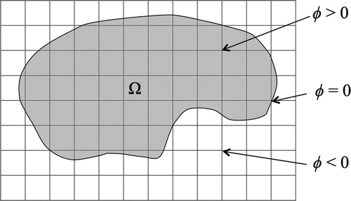
The first key component of level set based topology optimisation is to define the boundary of the structure as the zero level set of an implicit functionwhere Ω is the domain for the structure, Γ is the boundary of the structure, ϕ(x) is the implicit function and x ∈  Ω_d, where Ω_d is the design domain containing the structure, Ω ⊂  Ω_d, as shown in Fig. 2. The implicit function is a simple scalar function that has a value at each point in the domain. The domain is usually discretised such that the implicit function is only defined for a finite number of points within the design domain. It can then be interpolated between these points using shape functions in a similar manner to a FE discretisation.

2. Implicit description of structure

There are several optimisation methods that utilise an implicit description of the structure. In the present paper, the conventional level set method is used.²⁸ This approach initialises the implicit function as a signed distance function, where the magnitude of the function indicates the shortest distance to the boundary and the sign is defined by equation (1). Maintaining the signed distance property throughout the optimisation is important for the stability of the method, as it prevents the implicit function becoming too steep or flat, which can lead to numerical instabilities.⁴³

In the conventional level set method, the solution of the following advection equation is used to move the position of the implicit boundarywhere t is a fictitious time domain. The advection equation (2) becomes a Hamilton–Jacobi type equation by considering advection velocities of the type:⁴³ dx/dt = V ·▽ϕ (x), where V is a velocity function acting normal to the boundary. The equation is then discretised in space and time and solved using an explicit forward Euler scheme, producing the following update rule for the discrete implicit function valueswhere k is the iteration number, i is a discrete point in the design domain, Δt is the time step and V_i is the velocity value at the point i.

Fixed grid analysis

The level set method is usually performed on a fixed grid. For level set based structural optimisation, the same fixed grid is often also used for the FE discretisation. This approach avoids the difficult and expensive remeshing of the structure as the design changes during optimisation. However, some elements in the mesh may be cut by the boundary as the mesh is not fitted to the structure. To handle this situation, the area fraction weighted fixed grid approach is used,⁴⁴ where the properties of an element are multiplied by the fraction of the element that lies within the element:where E_i and ρ_i are the Young's modulus and density of the material for element i, the overbar denotes the effective material properties used to build the FE matrices and α_i is the area fraction, defined aswhere A_i is the total area of element i, and A_i,IN is the area of the element that lies inside the structure.

Sequential linear programming level set method

A general optimisation problem involves minimising an objective while satisfying equality and inequality constraints. In level set based optimisation, the velocity function should aim to maximise the reduction of the objective function while maintaining or improving the feasibility of the constraint functions. This can be achieved by defining the velocity function using the shape derivatives of the objective and constraint functions.⁴² The position and topology of the boundary is then updated using equation (3). The process of obtaining a velocity function and updating the implicit function is performed iteratively until a converged solution is obtained.

Shape derivatives are used to define the velocity function because they provide information about how a function changes over time with respect to a movement of the boundary. Shape derivatives usually take the form of a boundary integralwhere s_f is the shape sensitivity function for f(Ω). There are several approaches for obtaining an appropriate velocity function for optimisation. In the present work, the SLP level set method is used.⁴² There are two key steps in this method. The first is the discretisation of the shape derivative boundary integrals to produce simple approximations for the function changes with respect to a velocity function. For example, the discretisation of the integral in equation (6) can be written aswhere l_j is a discrete length of the boundary (or surface area in 3D) around a discrete boundary point j, s_f,j is a discrete value of the shape sensitivity function, n is the number of discrete points, V is a vector of discrete velocity function values and c is a vector of integral coefficients. Note that each side in equation (7) has been multiplied by the time step to produce the total change in f(Ω) after updating the implicit function.

The second step in the SLP level set method is to solve an optimisation subproblem to obtain a velocity function that minimises the objective function shape derivative, while maintaining constraint feasibility, or moving the constraints towards the feasible region. To produce solutions with smooth structural boundaries, it was found necessary to restrict the admissible velocity function to a linear combination of the shape sensitivity functions of the objective and constraintswhere λ are weights for each shape sensitivity function, and p is the total number of constraints. The subproblem is then to find the optimal weight values, which is solved using SLPwhere a_i and b_i are the integral coefficients for the equality and inequality constraints respectively, h_i and g_i are constraint change targets in the subproblem for constraint i, m is the number of equality constraints and p is the total number of constraints.

The SLP level set method offers a framework for handling general constraints for the conventional level set approach. A further benefit is that non-level set design variables can be easily introduced into the problem. This is achieved by including the first order derivatives of the non-level set design variables in the subproblem. The variables in the subproblem are then the change in the additional variables Δy and the velocity function for this iterationwhere y are the non-level set design variables, ▽f_y, ▽h_i,y, ▽g_i,y are the first order derivatives of the objective function, equality and inequality constraints with respect to y and Δy is the change in y for the current iteration. The non-level set design variables are then updated at the same time as the implicit function usingThe SLP level set method allows for simultaneous optimisation of the level set topology and other design variables making it an ideal tool for the simultaneous optimisation of topology and material distribution. This section has briefly covered the key concepts of the SLP level set method, for further details and numerical implementation (see Ref. 42). The extension of the SLP level set method for simultaneous topology and material design is introduced in the next section.

Material and topology optimisation

Material distribution model

The continuous distribution of two materials is modelled by specifying the fraction of one of the materials within each element in the fixed FE mesh. The stiffness and density of an element are then approximated using the simple rule of mixtures approachwhere y_i is the material design variable for element i, which can range continuously from 0 to 1, subscripts 1 and 2 refer to materials 1 and 2 respectively. The Poisson's ratio of the two materials may also be different. However, for the metallic materials considered in the present paper, this difference is small. Thus, a simplification is made where the Poisson's ratio of the material mix is assumed constant. To simultaneously optimise topology and material distribution, the material design variables y_i are added to the topology optimisation problem using the SLP level set method, as shown in equation (10).

Material design variable derivatives

The first order derivatives of the material design variables with respect to the objective and constraints are required to solve the subproblem for V and Δy in equation (10). The optimisation problem studied in the present paper is to minimise the structural compliance, which can also be understood as the work performed by the loading, with an upper limit on the total structural masswhere K is the global stiffness matrix, which is dependent on the structural domain described by the implicit function (equation (1)), and the material design variables y, f_s is the applied surface loading, f_b is the body force loading, u is the displacement vector, m is the mass of the structure, M is the limit on structural mass and C is the compliance of the structure. The derivatives of compliance and mass with respect to the structural domain are handled implicitly through shape derivatives and velocity function (equation (6)). Using the FE discretisation of the structure and the effective element material property definitions from equations (4) and (12), the terms dependent on y in equation (13) can be written aswhere ne is the total number of elements, K _e is the stiffness matrix of an element with E and α equal to 1·0, t_i is the thickness of a 2D element, κ _i is a vector of accelerations at each degree of freedom for element i and the factor of 1/4 in equation (16) is because four-node plane stress elements are used in the present work.

The derivative of the structural mass with respect to a single material design variable isThe adjoint method can be used to obtain the first order derivatives of the compliance objective with respect to the material design variables. It is well known that the compliance function is self-adjoint.⁷ Therefore, we omit the derivation and simply present the resultwhere u _i is the displacement vector for element i. The necessary partial derivatives can be obtained by differentiating equations (14) and (16)

Numerical issues

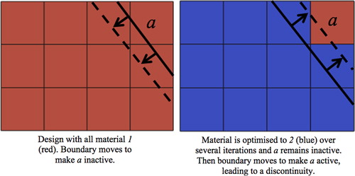
The approach introduced above uses one material design variable per element in the fixed FE mesh. However, the implicit structure description usually results in some elements in the fixed mesh lying completely outside the structure. Therefore, during the optimisation, some material design variables can become effectively inactive, as they do not affect the design. Inactive design variables are handled by removing them from the subproblem (equation (10)) and update (equation (11)). This approach is efficient as it reduces the number of variables in the subproblem. However, as the implicit boundary moves through the fixed grid, some elements that were completely outside the structure can become part of the structure. This can create a discontinuity in the optimisation if there is a discontinuity in the material distribution between an element that is part of the structure and an inactive element that becomes part of the structure during an update, as shown in Fig. 3. In the SIMP approach to combined topology and material optimisation, this type of discontinuity is less likely to occur, as all design variables are active throughout the optimisation.³² Also the use of sensitivity filtering may help smooth any potential discontinuities.

3. Discontinuity of material distribution caused by inactive design variables

This discontinuity is addressed by setting an inactive material design variable to the average of the active variables from neighbouring elements, as shown in Fig. 4. Inactive design variables are updated in this way at the same time as the update of the active design variables.

4. Setting material design variable for inactive element a

Examples

Three-dimensional cantilevered beam

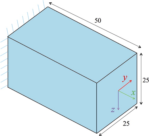
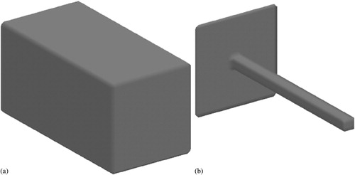
The first example is a 3D cantilevered beam. The design domain is discretised using 25 × 25 × 50 unit sized eight-node elements. The design domain, boundary conditions and load cases are shown in Fig. 5. The properties for material 1 are E₁ = 1·0, ρ₁ = 1·0, and for material 2, E₂ = 0·7, ρ₂ = 0·68. A Poisson's ratio of 0·3 is used for both materials. The objective is to minimise the compliance subject to a mass constraint of 1100 units. Three separate load cases are applied, one in each orthogonal direction at the loading point. The magnitude of the loads is 0·4, 20·0 and 20·0 in the x, y, and z directions respectively.

5. Cantilevered beam: design domain, loading and boundary conditions

The optimisation is run twice with two different initial designs to demonstrate the robustness of the level set topology optimisation method. The first starts with the entire design domain filled with material; the second starts with a thin beam (Fig. 6). The same solution is obtained from both starting points, as shown in Fig. 7. In each case, the design is composed of 100% of material 1. The compliance value for the two solutions is within 0·5%.

6. a full design domain; b thin beam

Initial designs

7. a from full design domain; b from thin beam

Optimum solutions

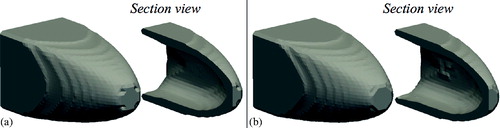
For this example, the optimal design does not contain material grading. However, it is unclear before the optimisation which of the two materials is the best choice, as material 1 has higher stiffness, whereas material 2 has higher specific stiffness. This example shows that by adding material design variables into the problem, the optimiser is able to determine the best material choice. This is confirmed by solving the topology optimisation problem using only material 2, which produces a solution with 13% higher compliance than the 100% material 1 solution.

This example also demonstrates that there are no fundamental limitations in applying the proposed optimisation method to design 3D structures with graded materials.

Two-dimensional cantilevered beam

A cantilevered beam of aspect ratio 1·6 is optimised with graded materials in this example. The design domain is discretised using 128 × 80 unit sized elements, which are 1 unit thick (Fig. 8). The properties for material 1 are E₁ = 100, ρ₁ = 1·0, and for material 2, E₂ = 150, ρ₂ = 1·4. A Poisson's ratio of 0·3 is used for both materials. The mass constraint for the problem is 5120 units.

8. Short cantilever: loading, boundary conditions and initial topology

Optimisation was run for four cases: case 1, using only material 1; case 2, using only material 2; case 3, simultaneous material and topology optimisation; and case 4, a sequential approach where the topology is optimised first for a fixed material distribution, then the material distribution is optimised for the converged topology. For the two problems that consider material distribution optimisation (cases 3 and 4), the starting value for all material design variables is 0·5 (an equal mix of the two materials). The final topology and material distributions for the four optimisation cases are shown in Fig. 9.

9. Cantilevered beam solutions: topology for a only material 1, b only material 2, c simultaneous topology and material optimisation, d sequential optimisation and material distribution for e simultaneous optimisation and f sequential optimisation

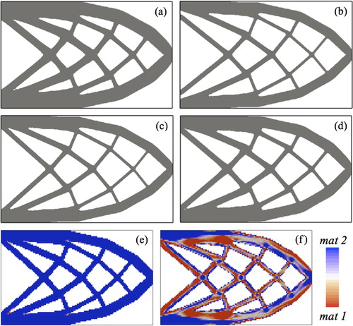
The final topology for all solutions is the same. However, structural dimensions are different in order to meet the mass constraint, as the materials have different densities. The final compliance values for the four solutions are 35·70, 32·14, 32·05 and 32·59, for only material 1, only material 2, simultaneous and sequential optimisation respectively. The maximum difference between optimum compliance values is only 11%, which suggests that, for this example, the topology is a more significant factor on the compliance than the material choice or distribution.

The solution obtained using the simultaneous approach has almost 100% of material 2 in the final design (Fig. 9e), and the topology and compliance of this solution are close to those obtained using only material 2 (Fig. 9b). These designs have slightly lower compliance than the solution obtained using the sequential approach, which is made from an even amount of each material. The sequential approach cannot obtain a solution with 100% of material 2 because the mass constraint is satisfied in the topology optimisation phase for an even mix of the two materials. Therefore, as the volume of material is fixed during the material optimisation phase, the solution for the sequential approach has the same even mix of the two materials. This demonstrates that the sequential approach can limit the exploration of the design space and the simultaneous approach is able to find the optimum solution that the sequential approach cannot.

It is interesting to observe in the sequential solution that islands of material 2 are present at the intersection of members in the lattice-like structure. This may be explained by the fact that two load paths run through an intersection and material 2 is the stiffer of the two materials. Therefore, the optimiser makes the choice of putting the stiffer material where the structure sees the highest loads to reduce the overall compliance. Moreover, there are areas in the sequential solution composed of a mixture of the two materials, which is of course permitted by the optimisation approach. Some areas appear composed of an even mix of the two materials, which is also the mixture for the initial design. However, these design variables change during optimisation and are not simply stuck at their initial values.

Beam with self-weight

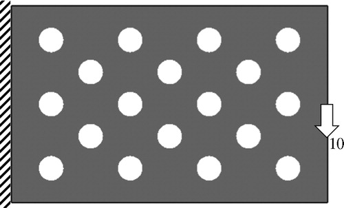
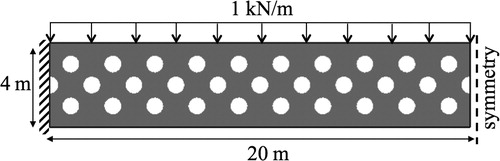
A clamped beam with a uniformly distributed load along the top is optimised for topology and materials. In addition, the self-weight of the beam is also considered during optimisation. Using symmetry conditions, only the left half of the beam is modelled (Fig. 10). The design domain is discretised using 400 × 80 square elements, which are 0·01 m thick. The properties for material 1 are E₁ = 70 GPa, ρ₁ = 2800 kg m^− 3, and for material 2, E₂ = 110 GPa, ρ₂ = 4500 kg m^–3. A Poisson's ratio of 0·3 is used for both materials. The mass constraint for the problem is 1250 kg. The four cases of material 1 only, material 2 only, simultaneous material and topology optimisation and sequential optimisation are studied, and the final topologies and material distributions for the full beam for all cases are shown in Fig. 11.

10. Beam with self-weight: loading, boundary conditions and initial topology

11. Beam with self-weight: topology for a only material 1, b only material 2, c simultaneous topology and material optimisation, d sequential optimisation and material distribution for e simultaneous optimisation and f sequential optimisation

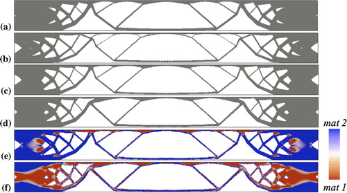
The final compliance values for the four solutions are 5·98, 5·36, 5·15 and 5·12 N m, for only material 1, only material 2, simultaneous and sequential optimisation respectively. The topologies for all solutions are similar. The best single material design is for material 2, which has 10% lower compliance than the solution for material 1. The two solutions that consider material distribution have compliance values within 1%, which is ∼4·5% lower than the material 2 solution. This shows that a design with material grading can obtain a lower compliance value than a single material design. However, for this example, the solutions using the simultaneous and sequential approaches obtain similar compliance values, although the percentage of each material in the final design is different. This suggests that there can be multiple optimum solutions. The percentage of material 2 for the simultaneous and sequential approaches solutions is 83 and 50% respectively.

Optimisation with uncertainty

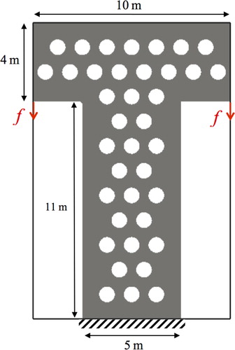
Real structures operate in an uncertain environment. Robust optimisation is one approach that considers uncertainties by optimising the stochastic performance of the design, such as the mean or variance. The example in this section minimises the mean, or expected compliance of a structure (Fig. 12) with uncertainties in the loading magnitude and direction. Normal probability distributions are assumed for the uncertainties, and the minimisation of expected compliance problem can be reformulated as a simpler multiple load case problem.⁴⁵ The probability distributions for both applied loads f are the same. The mean magnitude is 10 kN, and standard deviation is 2 kN. The standard deviation for the uncertain direction is 0·25 rad. The design domain is discretised using 100 × 150 elements, which are 0·01 m thick. The properties for material 1 are E₁ = 70 GPa, ρ₁ = 3000 kg m^− 3, and for material 2, E₂ = 120 GPa, ρ₂ = 5000 kg m^− 3. A Poisson's ratio of 0·3 is used for both materials. The mass constraint for the problem is 1500 kg. The final topology and material distributions for all cases are shown in Fig. 13.

12. Optimisation problem with uncertain loading

13. Uncertain loading solutions: topology for a only material 1, b only material 2, c simultaneous topology and material optimisation, d sequential optimisation and material distribution for e simultaneous optimisation and f sequential optimisation

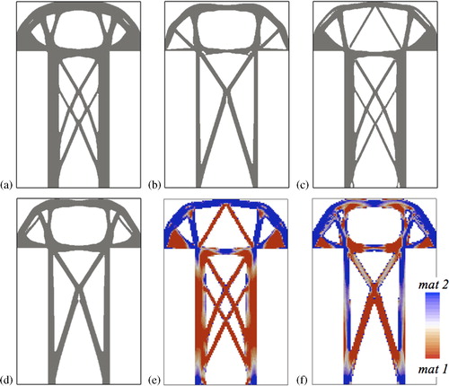
The expected compliance for the four solutions are 10·48, 9·92, 9·49 and 9·87 N m, for only material 1, only material 2, simultaneous and sequential optimisation respectively. Both solutions that consider material distribution obtain a lower expected compliance compared with the single material designs. The best result is obtained using the simultaneous optimisation approach, which has an expected compliance value ∼4% lower than the solution obtained using the sequential approach. It is noticeable in this example that the topologies of the four solutions are different, although there are some similar features, such as the cross-bracing of the central column. This demonstrates how material choice and optimisation strategy can affect the optimal topology.

Conclusions

A new level set method is introduced for simultaneously optimising the topology and continuous material distribution of a structure. The topological solutions are represented by smooth boundaries, which make them naturally suited for AM. The distribution of two materials is modelled by specifying the fraction of one of the materials within each element in the fixed FE mesh. These fractions become additional design variables in the optimisation problem. The topology and material distribution are optimised simultaneously using the SLP level set method.

The examples demonstrate that the optimisation method is robust in converging to the consistent optimum solution. Solutions obtained by the proposed method are compared against those using a single material and a sequential approach, where topology is optimised first, followed by material distribution optimisation. It has been shown that the simultaneous material and topology optimisation approach is able to explore the largest design space, hence has the potential to find the global optimum. The results also suggest that there may be multiple optimum solutions due to the expanded design space, and this can offer engineers an opportunity to select from a range of optimum solutions. The last example establishes that it is possible for optimum solutions to account for uncertainties in the design environment.

Acknowledgements

The authors acknowledge the support from Engineering and Physical Sciences Research Council, grant number EP/M002322/1.The authors would also like to thank the Numerical Analysis Group at the Rutherford Appleton Laboratory for their FORTRAN HSL packages (HSL, a collection of Fortran codes for large scale scientific computation; see http://www.hsl.rl.ac.uk/).

References

- Muir M. J., Toropov V. V. and Querin O. M.: ‘Rules, precursors and parameterization methodologies for topology optimized structural designs realized through additive manufacturing’, Proc. Conf. AIAA SciTech 2014, National Harbor, MD, USA, January 2014, AIAA, 1–11.
- Brackett D., Ashcroft I. and Hague R.: ‘Topology optimization for additive manufacturing’, Proc. 24th Solid Freeform Fabrication Symp., Austin, TX, USA, August 2011, University of Texas at Austin, 6–8.
- Leary M., Merli L., Torti F., Mazur M. and Brandt M.: Mater. Des., 2014, 63, 678–690.
- Doubrovski Z., Verlinden J. C. and Geraedts J. M.: ‘Optimal design for additive manufacturing: opportunities and challenges’, Proc. ASME 2011 International Design Engineering Technical Conf. and Computers and Information in Engineering Conf., Washington, DC, USA, August 2011, American Society of Mechanical Engineers, 635–646.
- Harzheim L. and Graf G.: Struct. Multidiscip. Optim., 2006, 31, (5), 388–399.
- Haftka R. T. and Gürdal Z.: ‘Elements of structural optimization’; 1992, London, Kluwer Academic.
- Bendsoe M. P. and Sigmund O.: ‘Topology optimization: theory, methods and applications’; 2004, Berlin, Springer-Verlag.
- Zhou M., Shyy Y. K. and Thomas H. L.: ‘Topology optimization with manufacturing constraints’, Proc. 4th World Cong. on ‘Structural and multidisciplinary optimization’, Dalian, China, June 2001, International Society for Structural and Multidisciplinary Optimization.
- Harzheim L. and Graf G.: Int. J. Veh. Des., 2002, 28, (4), 389–409.
- Xia Q., Shi T., Wang M. Y. and Liu S.: Struct Multidiscip. Optim., 2010, 41, (5), 735–747.
- Leiva J. P., Watson B. C. and Kosaka I.: ‘An analytical bi-directional growth parameterization to obtain optimal castable topology designs’, 10th AIAA/ISSMO Multidisciplinary Analysis and Optimization Conf., Albany, NY, USA, August-September 2004.
- Tang P. S. and Chang K. H.: Struct Multidiscip. Optim., 2001, 22, (1), 65–82.
- Hsu M. -H. and Hsu Y. -L.: Comput. Struct., 2005, 83, (4-5), 327–337.
- Challis V. J., Roberts A. P., Grotowski J. F., Zhang L. C. and Sercombe T. B.: Adv. Eng. Mater., 2010, 12, (11), 1106–1110.
- Gaynor A. T., Meisel N. A., Williams C. B. and Guest J. K. J.: Manuf. Sci. Eng., 2014, 136, (6), 061015.
- Andreassen E., Lazarov B. S. and Sigmund O.: Mech. Mater., 2014, 69, (1), 1–10.
- Schwerdtfeger J., Wein F., Leugering G., Singer R. F., Korner C., Stingl M. and Schury F.: Adv. Mater., 2011, 23, (22–23), 2650.
- Muir M. J., Toropov V. V. and Querin O. M.: ‘Civil aerospace mass reduction through automated topology optimization and advanced manufacturing’, Proc. ASMO UK/ISSMO Conf. on ‘Engineering design optimization’, Cork, Ireland, July, 2012, American Institute of Aeronautics and Astronautics, 111–127.
- Bendsoe M. P.: Struct. Optim., 1989, 1, (4), 193–202.
- Bendsoe M. P. and Kikuchi N.: Comput. Meth. Appl. Mech. Eng., 1988, 71, (2), 197–224.
- Querin O., Young V., Steven G. and Xie Y.: Comput. Meth. Appl. Mech. Eng., 2000, 189, (2), 559–573.
- Sigmund O. and Petersson J.: Struct. Optim., 1998, 16, (1), 68–75.
- Kim H., Querin O. M. and Steven G. P.: Evol. Des. Manuf., 2000, 33–44.
- Eschenauer H. A., Kobelev V. V. and Schumacher A.: Struct. Optim., 1994, 8, (1), 42–51.
- Lee S., Kwak B. M. and Kim I. Y.: Int. J. CAD/CAM, 2007, 7, (1)
- Edwards C. S., Kim H. A. and Budd C. J.: ‘Smooth boundary based optimisation using fixed grid’, Proc. 7th World Cong. on ‘Structural and mulidisciplinary optimization’, Seoul, Korea, May 2007, COEX, 1789.
- van Dijk N. P., Maute K., Langelaar M. and van Keulen F.: Struct. Multidiscip. Optim., 2013, 48, (3), 437–472.
- Deaton J. D. and Grandhi R. V.: Struct. Multidiscip. Optim., 2014, 49, (1), 1–38.
- Gain A. L. and Paulino G. H.: Struct. Multidiscip. Optim., 2013, 48, (4), 685–710.
- Yin L. and Ananthasuresh G. K.: Struct. Multidiscip. Optim., 2001, 23, (1), 49–62.
- Hiller J. D. and Lipson H.: ‘Multi material topological optimization of structures and mechanisms’, Proc. 11th Annual Conf. on ‘Genetic and evolutionary computation’, Montreal, Canada, July 2009, ACM, 1521–1528.
- Sigmund O. and Torquato S. J.: Mech. Phys. Solids, 1997, 45, (6), 1037–1067.
- Gibiansky L. V. and Sigmund O. J.: Mech. Phys. Solids, 2000, 48, (3), 461–498.
- Paulino G. H., Silva E. C. N. and Le C. H.: Struct. Multidiscip. Optim., 2009, 38, (5), 469–489.
- Zhou S. W. and Wang M. Y.: Struct. Multidiscip. Optim., 2007, 33, (2), 89–111.
- Wang M. Y. and Wang X.: Comput. Meth. Appl. Mech. Eng., 2004, 193, 469–496.
- Sigmund O.: Comput. Meth. Appl. Mech. Eng., 2001, 190, (49–50), 6605–6627.
- Guest J. K.: Comput. Meth. Appl. Mech. Eng., 2009, 199, (1–4), 123–135.
- Brice C. A., Newman J. A., Bird R. K., Shenoy R. N., Baughman J. M. and Gupta V. K.: ‘Electron beam freeform fabrication of titanium alloy gradient structures’, NASA/TM-2014-218508, NASA, NASA Langley Research Center; 2014, Hampton, VA, USA
- Zhang Y. Z., Wei Z. M., Shi L. K. and Xi M. Z. J.: Mater. Process. Technol., 2008, 206, (1–3), 438–444.
- Dunning P. D., Stanford B. K., Kim H. A. and Jutte C. V. J.: Fluids Struct., 2014, 292, 312.
- Dunning P. D. and Kim H. A.: Struct. Multidiscip. Optim., 2015, 51, (3), 631–643.
- Sethian J. A.: ‘Level set methods and fast marching methods’; 1999, New York, Cambridge University Press.
- Dunning P. D., Kim H. A. and Mullineux G.: Finite Elem. Anal. Des., 2011, 47, (8), 933–941.
- Dunning P. D., Kim H. A. and Mullineux G.: AIAA J., 2011, 49, (4), 760–768.